1. Introduction
The intelligence level of an unmanned surface vehicle (USV) has been improved a lot in recent years; however, it is still challenging to achieve a precise motion planning for USVs in complex environments [
1,
2,
3]. Due to the particularity of USV navigation environments, it is inevitable that USVs will be affected by the wind, wave, current and other environmental factors in the navigation process. Therefore, it is necessary to consider the impact of environmental factors, where the efficiency and safety of task implementation by the USV need to be taken into account. As far as we know, no previous research has investigated the effects of wind and current on USV motion planning from the perspectives of USV dynamics and cyber-physic systems. In order to fill this gap, we particularly need to figure out how to avoid the adverse influence of wind and current on motion planning for a USV in complex environments, which is one of the key problems that should be solved in the process of USV intelligentization [
4].
Although many researchers focus on USV motion and path planning in complex environments [
5,
6,
7,
8,
9,
10,
11,
12,
13], there are still some problems that need to be solved with respect to the influence of actual wind and current dynamics on USV motion planning. For example, from the perspectives of USV navigation characteristics and cyber-physic systems: How do the wind and current disturb the distance and direction of the USV in the motion planning process? How do the wind and current disturb USV steering in the motion planning process? It is necessary to take these two problems into account during USV navigation. In particular, it is more critical to consider the influence of wind and current on the dynamics of the USV and how the dynamics of the USV changes in the process of motion planning.
The remainder of this paper is organized as follows: an analysis of related works is introduced in
Section 2; a major issue and methodology are presented in
Section 3; a USV mathematical motion model in terms of wind and current effects is provided in
Section 4; the construction of time-varying trajectory cells is presented in
Section 5; on the basis of time-varying trajectory cells, regularization-trajectory cells that take into account wind and current effects are also provided in
Section 5; a USV motion planning method with respect to wind and current effects is introduced in
Section 6; simulation experiments and analyses are introduced in detail in
Section 7; the conclusion and outlook of the paper are given in
Section 8.
2. Related Works
Path planning, with the effects of wind and current taken into consideration, needs to be optimized from different perspectives such as the distance of the path, the safe path, and the smooth path. Much research has been performed to help solve the USV motion planning problem with the effects of wind and current.
Singh et al. [
5] proposed a method on the basis of the A* algorithm [
14] to solve the USV path planning problem under the influence of the current. This method mainly projects the planning map to a binary electronic map, in which they set the safety distance between the USV and the obstacle as a certain pixel according to the constraint pixels of the electronic map; it then solves the problem of path planning under the influence of the current. To a certain extent, it provides useful inspirations for solving the path planning problem of the current affecting the USV since they considered the path distance and safety of the planned route.
Ma et al. [
6] provided a multi-objective optimization method for the influence of fixed current field and time-varying current field USV path planning. In this method, the multi-objective particle swarm optimization algorithm [
15] is constructed. The safety, economy, distance, and smoothness of the path are taken as the objective variables, and then the current function [
16,
17] is constructed as the environmental variables in order to realize path planning for a USV in the time-varying current field environment. They considered the safety, economy, distance, and smoothness of the planning path.
Thakur et al. [
7] proposed the state transition model of GPU to simulate a USV’s trajectory planning and then realized this trajectory planning in complex sea conditions. Li et al. [
18] researched the dynamics and kinematics model of a USV, simplified it according to the characteristics of a USV trajectory, proposed a three degrees-of-freedom motion model for USV navigation, and then further verified the effectiveness of the designed USV trajectory through simulation. However, Thakur and Li et al. [
7,
18] ignored the specific dynamic constraints of the USV.
Song et al. [
8] analyzed a fast marching algorithm [
19,
20] to solve the route planning problem of a USV facing a fixed current field, and then constructed a double-layer fast marching algorithm to realize a safe and economic route planning for a USV under the influence of a fixed current field. Song et al. [
9] improved the fast marching algorithm based on reference [
8] and designed the multi-layer fast marching algorithm in order to consider the time-varying current field route planning of USVs. References [
8,
9] also considered the safety and distance of the planning path. Oren et al. [
10] proposed a velocity obstacle method for path planning in response to wave disturbances while the USV is sailing in complex sea conditions. In their algorithm, the waves disturbing the USV are regarded as moving obstacles, and the velocity obstacle method based on probability prediction [
21] is constructed to realize USV path planning. This method provides some reference ideas for solving the navigation problems of a USV in complex sea conditions and has certain practical significance. More specifically, with regard to planning behavior, they considered some constraints such as USV size, and they also considered the safety and distance of the planned path. Based on the Voronoi-Visibility roadmap method and the ant genetic algorithm, Niu et al. [
11] proposed the optimal energy path planning method for USVs in the environment of the time-varying current field. They established a Voronoi visibility roadmap and combined it with a genetic algorithm to achieve the optimal energy path in a time-varying environment. Experiments indicate that their method’s performance is better than other methods.
Subramani et al. [
12] developed a path planning method for strong current environments; they mainly considered the influence of a time-varying environment by establishing partial differential equations and then constructed a navigable area in a time-varying environment by using a probability model. The method mainly considers time-varying optimal path planning under the influence of a strong current environment. However, their method cannot guarantee path planning safety since the probability of navigation points cannot be fully computed in a real-time system. The work most related to our study is that of [
13]; in our method, regularization-trajectory cells are developed to take into account the effects of wind and current, and we focus more on trajectory analysis with respect to wind and current effects, which can help in fully considering the USV characteristics.
3. A Major Issue and Methodology
In this section, we will analyse the influence of wind and current on USV motion planning with an experiment, and provide our methodology for USV motion planning considering wind and current effects.
Du et al. [
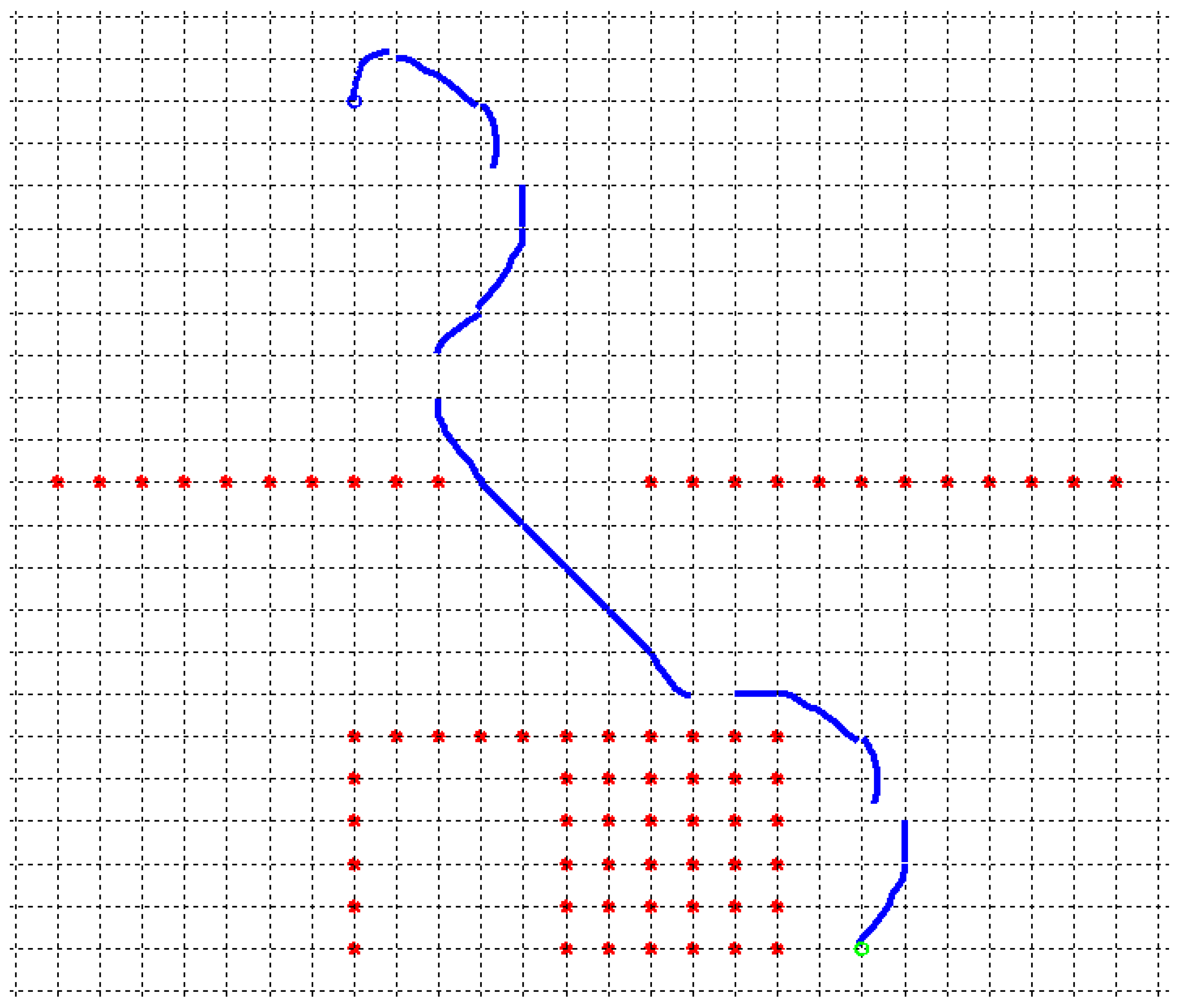
22] developed a trajectory-unit method for USV motion planning that considers the dynamic constraints of the USV. This method works well when USVs are not disturbed by wind and current. However, as shown in
Figure 1, the method can not provide good performance in complex environments, it does not consider the impact of wind and current on the dynamics of the USV. If the wind and current disturbances are considered in their method, the planned path will not be spliced. The reasons for this problem are: (1) its search algorithm does not consider environmental factors; (2) its trajectory unit does not consider environmental factors. When the environment changes, the trajectory unit becomes irregular and cannot adapt to complex environments; hence, it cannot effectively make the USV navigate in complex environments.
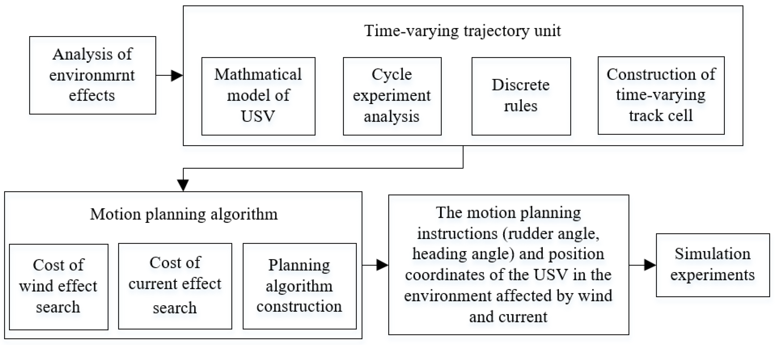
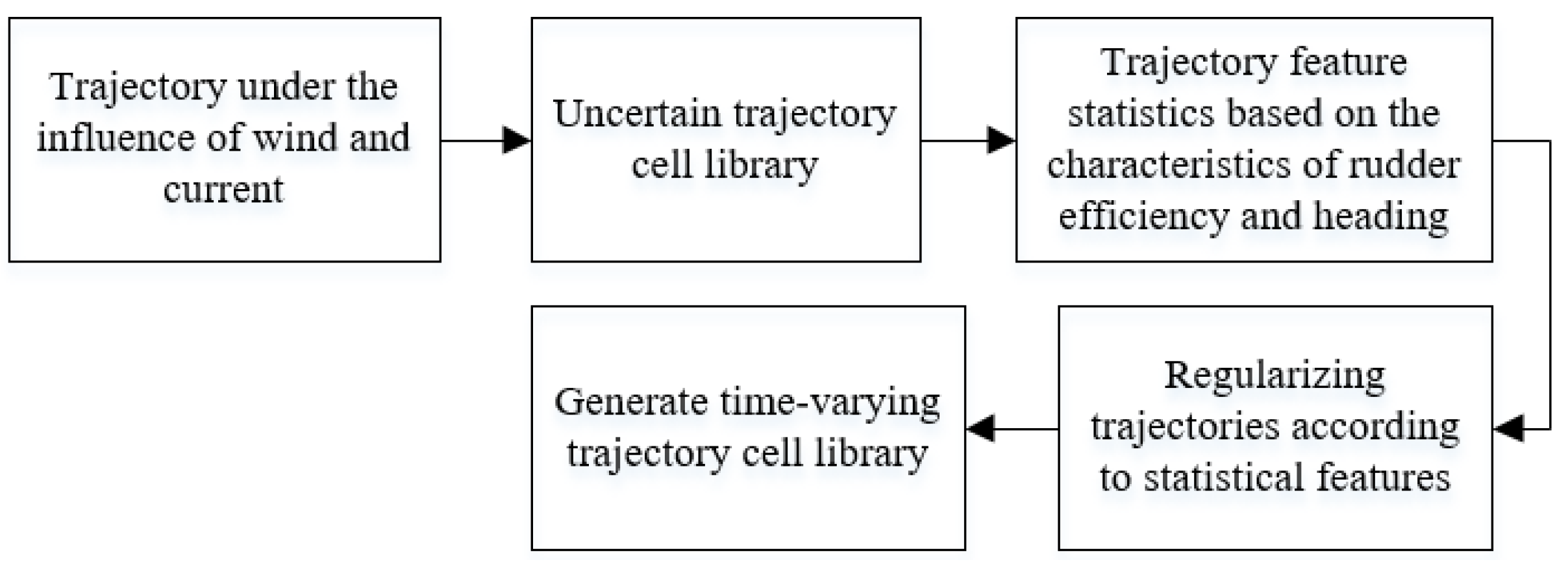
In order to solve this issue, a USV motion planning method based on the regularization-trajectory cell is proposed (as shown in
Figure 2). More specifically, first, a model is built under the influence of wind and current while considering the dynamics of the USV. Second, a regularization-trajectory cell based on the dynamics of the USV is constructed, taking into account the actual dynamics of the USV in the process of determining how to realize path planning. Third, after computing the impact of wind and current on the dynamics of the USV, an effective algorithm for USV motion planning is proposed to achieve an efficient, safe, and economical path search. In the next section, we will introduce a USV mathematical motion model that will play an important role in USV motion planning.
4. A USV Mathematical Motion Model
In this section, we establish the mathematical model of a USV that is exposed to wind and current disturbances, and the motion characteristics of the USV under the influence of environmental factors such as wind and current are further analyzed.
In the process of establishing the mathematical model of the USV, it is assumed that mainly the forward (x), traverse (y), and bow (n) of the USV are considered.
Therefore, the mathematical model of the USV here is given by Equation (
1):
In Equation (
1),
I,
H,
P,
R, and
respectively represent the forces (moments) generated by inertia, viscosity, propeller, rudder, and wind. A detailed introduction to the inertial model, viscous model, propeller model, and rudder model of a USV can be found in references [
22,
23,
24,
25].
4.1. Wind Disturbances
When the wind on the sea surface changes randomly, wind force disturbances are also random. Here, the wind on the sea surface is assumed to be uniform,
denotes the absolute wind speed,
denotes the direction of the absolute wind speed,
denotes the relative wind speed,
denotes the direction of the relative wind speed, and
denotes the USV speed. The absolute wind speed and direction are calculated in a geodetic coordinate system, and the relative wind speed and direction are calculated in a USV coordinate system [
26,
27].
The relationship between the absolute wind speed, relative wind speed, and USV speed is as follows:
We map this relationship to the USV-following coordinate system:
where
and
are the components on the
and
axes of the USV-following coordinate system. In the relative coordinate system, when the wind is blowing from the port side of the USV, the relative wind speed
and direction
are positive, and the calculated relative wind speed
and direction
are as follows:
The relative wind speed value obtained from this formula is:
where
is the drift angle.
4.1.1. Wind Pressure
The wind pressure and wind ballast calculated from the formula above are as follows.
The calculated forces and moments acting on the hull wind can be expressed as:
In the formula above, denotes air density, denotes the length of the USV, denotes the forward projection area of the USV’s water part, denotes the side projection area of the USV’s water part, denotes the wind pressure coefficient in the -axis direction, is the wind pressure moment coefficient in the -axis direction, and denotes the wind pressure coefficient in the y-axis direction.
The forward projection area and the side projection area need to be calculated in detail according to the general layout of the USV; in the absence of a detailed general layout of the USV, it can be roughly calculated according to reference [
28].
In addition, we calculate the wind pressure
(the coupling of different wind directions is considered in the calculation of wind pressure):
in Formula (7) is the coefficient of the wind pressure resultant force. According to the wind pressure resultant force, the moment in the
x-axis,
y-axis, and
z-axis is decomposed. By combining these formulas, the relationship of the wind pressure coefficients in each direction can be obtained:
where
is the position point of the pressure resultant force by wind, and
is the angle of the wind pressure resultant force.
4.1.2. Calculation of Wind Pressure and Moment
Generally, these correlation coefficients are obtained from a wind tunnel test. However, due to the limited experimental conditions and the impossibility of wind tunnel testing for every USV, this paper calculates the correlation coefficients according to the approximate calculation formulas given by A. Iwai and H. Kugumiya, and it is estimated for a general cargo ship [
28].
where
is the length between the perpendiculars of the ship; the wind force disturbances can be obtained according to the correlation coefficients calculated by the formulas above.
4.2. Current Disturbances
In the actual navigation process, it is assumed that the effect of the current on the ship can make the ship’s speed and direction deviate [
6]. Therefore, the effect of the current will change the
x-axis and
y-axis speed of the USV. To consider current disturbances, velocity is directly superimposed onto the ship’s velocity. As shown in Formula (12), where
u denotes transverse velocity after consideration of the current disturbances,
v denotes the longitudinal velocity after consideration of the current disturbances,
denotes the transverse velocity of the USV,
denotes the transverse velocity of the current,
denotes the longitudinal velocity of the USV, and
denotes the longitudinal velocity of the current.
5. Construction of Time-Varying Trajectory Cells
5.1. Analysis of the USV Turning Experiment
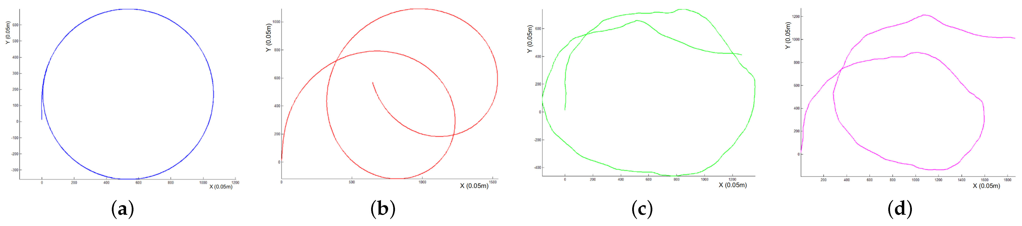
Disturbances by wind and current, dynamic constraints, state constraints, and other characteristics of environmental disturbances need to be considered from the perspectives of USV navigation characteristics and cyber-physic systems. Thus, this paper establishes a USV dynamics model under of wind and current disturbances, and based on a force analysis of the USV, we further analyze how the wind and current affect the navigation state of a USV in detail. The simulation experiments are carried out according to our trajectory analysis. The trajectory of the USV motion state without environmental disturbances, the trajectory of the USV motion state affected by the current, the trajectory of the USV motion state affected by the wind, and the trajectory of the USV motion state affected by wind and current at the same time are shown as follows.
As shown in
Figure 3a, there are no environmental disturbances in which the angle of the turning rudder is 12.5°. It is obvious that when there are no environmental disturbances, the results of the USV cycle meet actual needs. As shown in
Figure 3b, there are current disturbances of 1 m/s in the
x-axis direction and 1 m/s in the
y-axis direction, and in which the angle of the turning rudder is 12.5°; at this time, the turning path is shifted, and with the current disturbances, the turning trajectory becomes irregular.
Figure 3c is the result of the turning experiment of a USV, with a wind speed of 2 m/s and a wind direction of true north, and in which the angle of the turning rudder is 12.5°; in this experiment, the turning experiment trajectory of the USV becomes irregular due to the disturbances of the wind, resulting in an irregular cycle. As shown in
Figure 3d, the current velocity is 1 m/s in the
x-axis direction and 1 m/s in the
y-axis direction. The turning experiment is conducted with disturbances of wind speed of 2 m/s in the true north direction, in which the angle of turning rudder is 12.5°; in this experiment, the turning trajectory of the USV is irregular because of the superposition effect of the current and wind, and the force direction and force of the USV are constantly changing, which makes it challenging to predict the trajectory.
5.2. Rules of Time-Varying Trajectories
From these experimental results, when the USV is affected by the wind and current at the same time, the trajectories of the USV show irregular changes. However, the trajectory cell constructed in references [
22,
23] is a regular trajectory, which is not suitable for the motion planning of a USV with environmental disturbances. Thus, we established a regularization-trajectory cell, which lays the foundation for USV motion planning that takes into consideration the effects of both wind and current.
In this study, the influence of environmental factors is considered, and the rudder angle of the regularization-trajectory cell in this paper needs to be changed at any time through the search algorithm in order to maintain safe USV navigation. Therefore, the rudder angle of the regularization-trajectory cell in this paper is mutable, and it needs to be adjusted according to the environment change. Similar to references [
22,
23], to facilitate the consideration of the forces and moments on the USV, the following rules need to be considered in the construction of regularization-trajectory cells:
Rule 1: The trajectory cells are divided into 36 categories, and the trajectory distances of each category are equal within a certain error range. Based on this, a regularization-trajectory cell library is constructed.
Because environmental factors such as wind, wave, and current are changing at every moment, the 36 categories of the regularization-trajectory cells are built according to the search direction of the algorithm. There is a large number of regularization-trajectory cells in each category, that is, each category of regularization-trajectory cells can form a sub-regularization-trajectory cell library, which can provide sufficient reachable areas for USV motion planning.
Rule 2: In order to maintain the continuity of the search path, the motion state of the regularization-trajectory cell at the beginning and at the end is kept stable.
Rule 3: In the case of wind and current disturbances in a certain trajectory cell at a certain time, it is necessary to turn the rudder only once in order to continue with navigation, excluding a rudder’s return (steering to counteract the disturbances of the wind and current).
To sum up, the three rules specified in this section will lay the foundation for subsequent motion planning, which can better help to realize motion planning while considering environmental influences and USV navigation characteristics.
5.3. Regularization-Trajectory Cells
On the basis of the establishment of trajectory rules, in the grid environment, trajectories need to be constantly adjusted with the rudder angle to make the trajectory meet different navigation requirements based on the reachable points, the trajectory cell heading, and the final state of the trajectory cells. In addition, after generating the regularization-trajectory cells, for the convenience of calculation, the regularization-trajectory cells of the USV are divided into 36 categories, as mentioned above.
5.3.1. Regularization-Trajectory Cell Construction Method
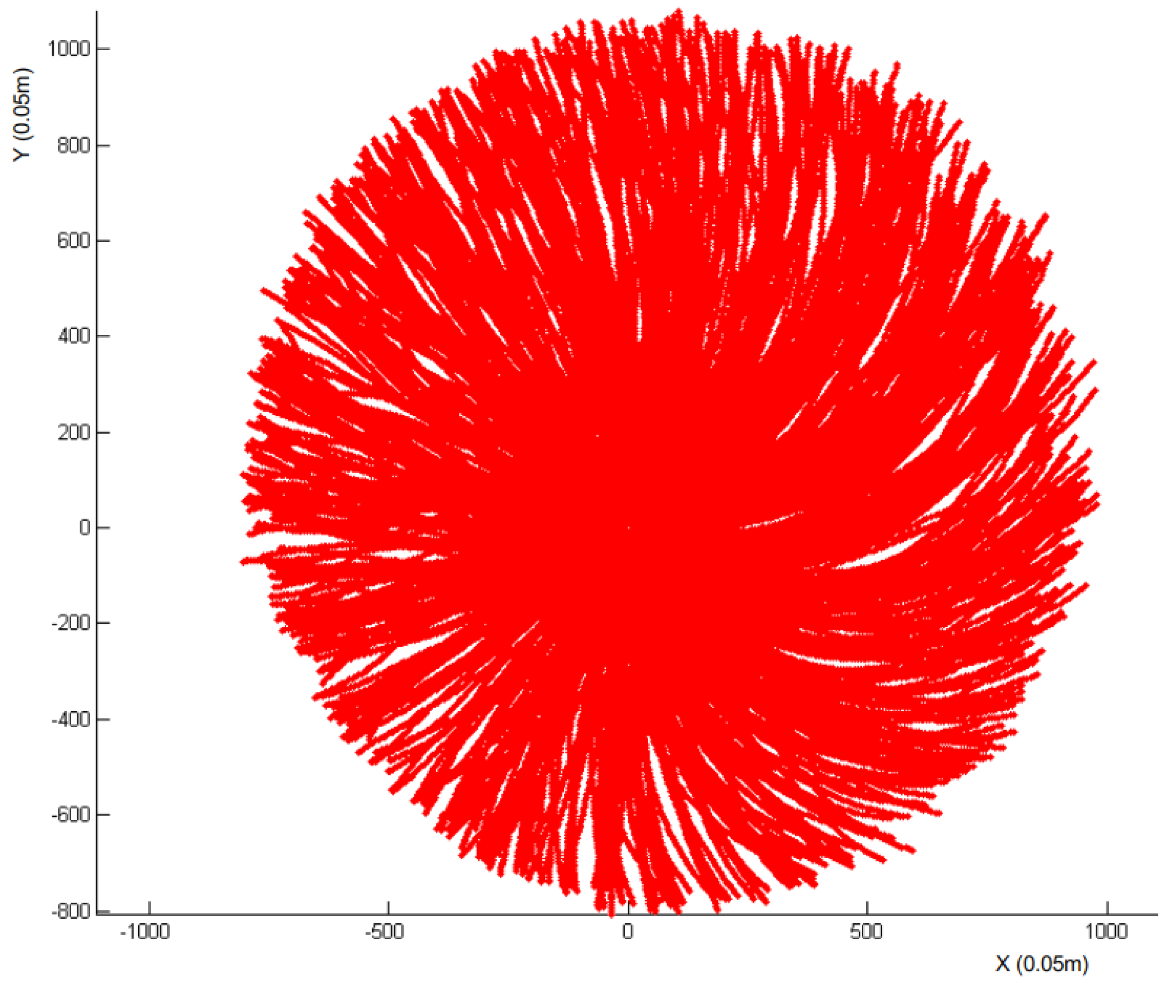
Based on the dynamics model of the USV under the influence of wind and current, the regularization-trajectory cell is constructed on the premise of the regular constraints of the regularization-trajectory cell. First of all, we explore the same rudder angle in different directions, as shown in
Figure 4, and search for the reachable points at 0.5° intervals (i.e., change the trajectory cell at 0.5° intervals, and the rudder angle at this time is 15°). It can be seen that the search area of the current point can be covered with full probability by exploring different heading intervals for the same rudder angle; thus, the full probability search can be realized.
According to the above-mentioned total probability exploration of the surrounding nodes, when the fixed trajectory cell [
29,
30] cannot be spliced, the established regularization-trajectory cell can be used (the trajectory cell changes according to the change of environments).
Figure 5 shows the chart for building a regularization-trajectory cell, which comprises of the USV geometry shape and physical characteristics. First, determine the current environmental information, that is, wind and current will have important disturbances on the trajectory cell; second, by building the uncertain trajectory cell library under the influence of wind and current, judge the characteristics and construct the corresponding trajectory cell; finally, resist the environmental disturbances by steering the rudder, that is to say, regularize the trajectory by changing the rudder angle in order to lay a foundation for the trajectory cell to achieve splice.
5.3.2. Building a Regularization-Trajectory Cell Library
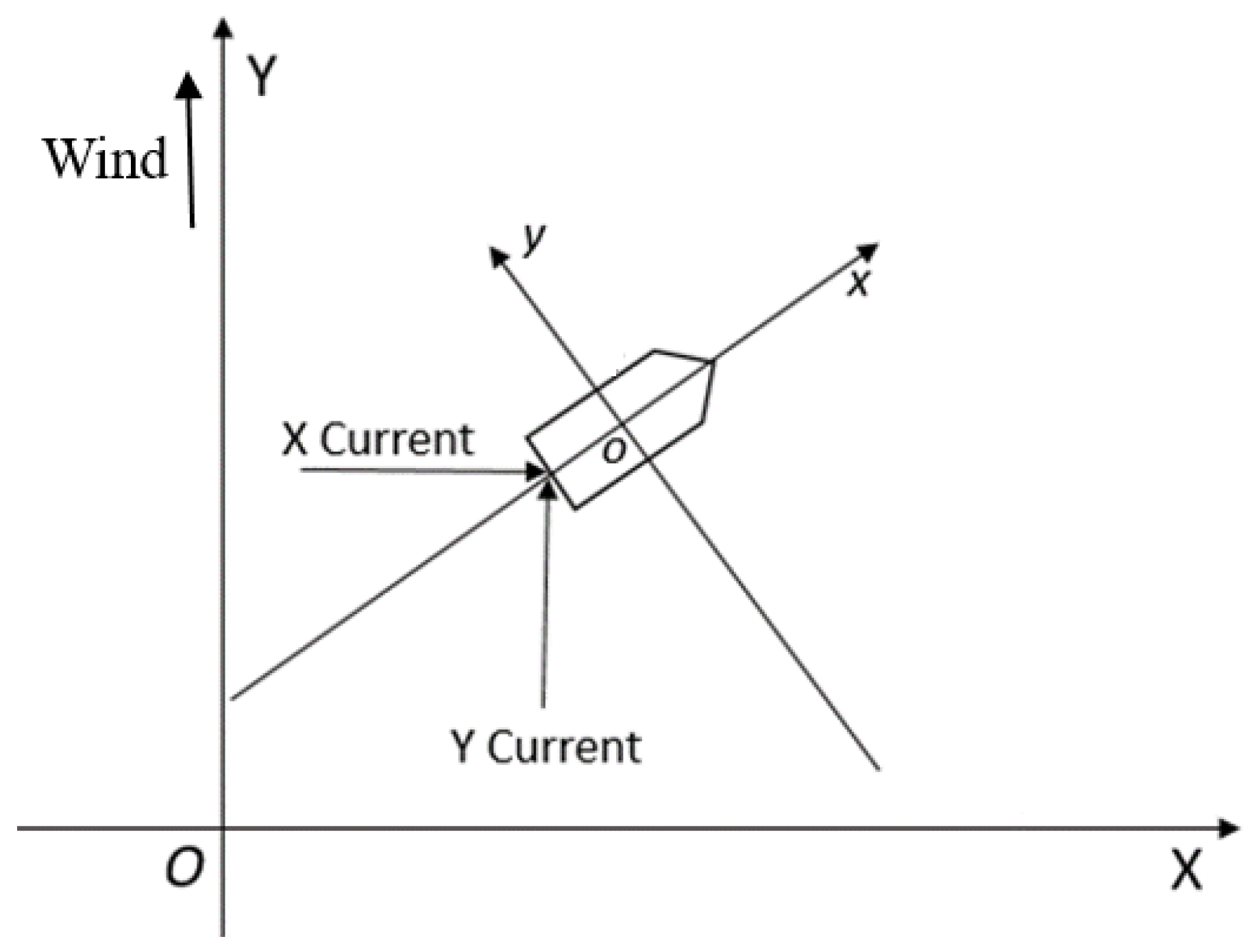
In this section, based on real-world environments, assume that the wind speed is 2 m/s and the wind direction is 0° (
Figure 6 shows a schematic diagram of ship motion under the influence of wind and current). Assume that the current speed in the
x-axis direction is 1 m/s and the current speed in the
y-axis direction is 1 m/s (the calculation of wind speed and current velocity here is based on the absolute wind speed and current speed, that is, the calculation is carried out in the fixed coordinate system).
6. Motion Planning Method
The trajectory rules and regularization-trajectory cells lay a solid foundation for the following planning method. In this section, based on the regularization-trajectory cell, motion planning for a USV under the influence of wind and current is further realized, which is derived from the A* algorithm.
First, we analyze the effects of wind and current, and then we generate the regularization-trajectory cell according to the influencing factors of wind and current. Second, we splice the trajectory cell under the influence of the environment according to the trajectory rules. We further adjust the path search generation value and the regularization-trajectory cells of the A* algorithm in real time on the basis of the influence of the environments, and we fully consider the motion rules of the USVs under the influence of wind and current. Finally, we construct the motion planning method of the USV under the influence of wind and current on the basis of the search algorithm and the regularization-trajectory cells. Based on this method, not only can the influence of wind and current be considered, but the influence of wave and other complex environments on the path planning of the USV can also be analyzed in more detail in the future.
6.1. Analyze Effects of Wind and Current
6.1.1. Analysis of Wind Effects
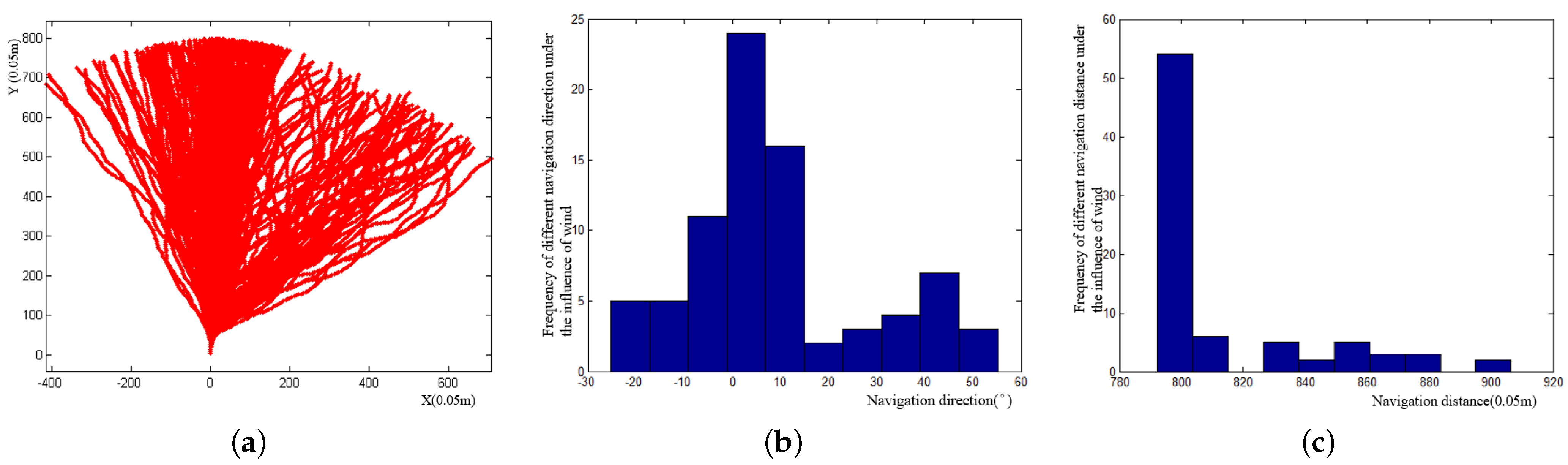
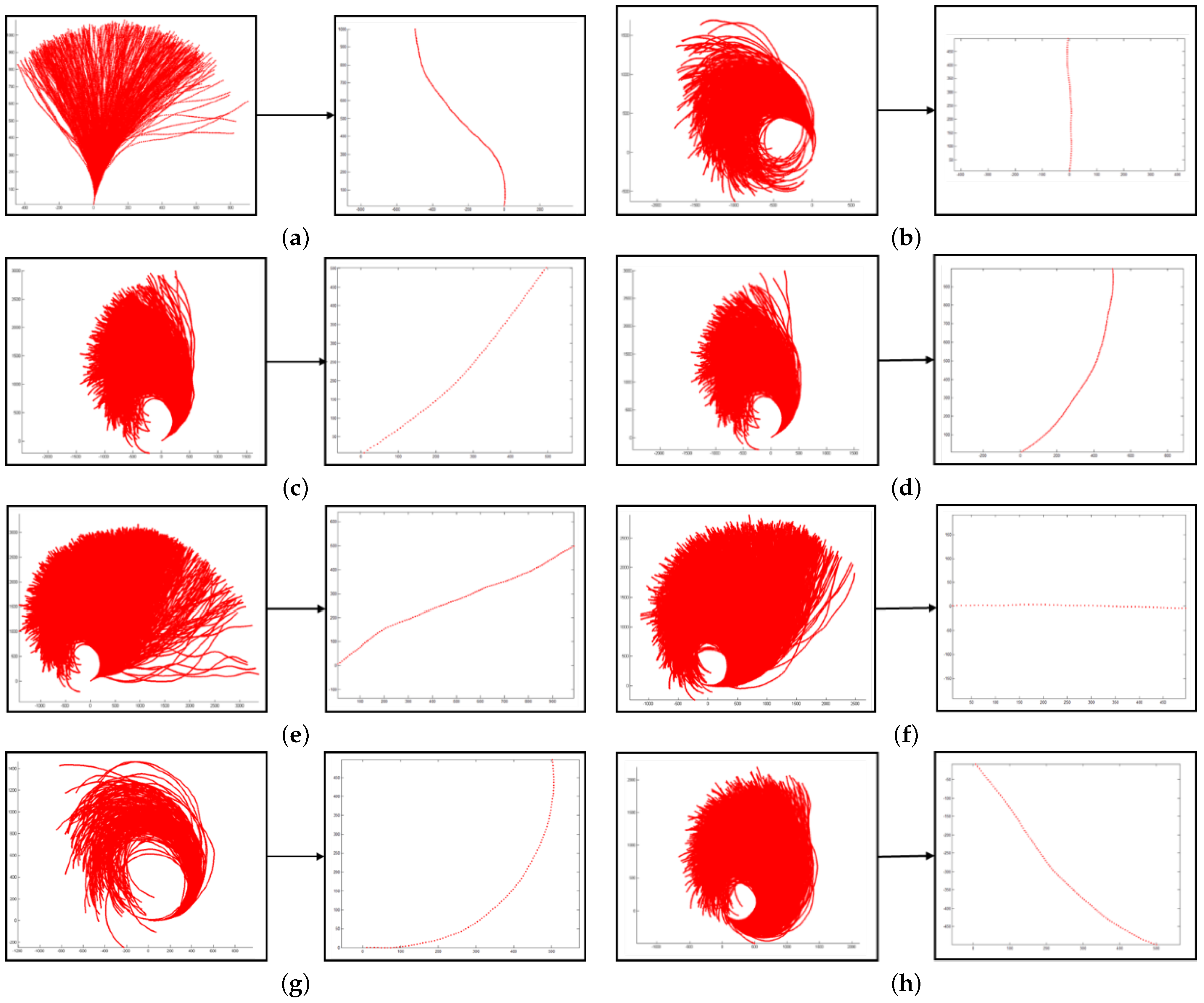
In this simulation experiment, the experimental wind speed is under normal conditions (0–8 m/s). According to the experimental results in
Figure 7, under the influence of a wind speed of 0–8 m/s after a certain period of navigation, the navigation distance of the USV is almost unchanged, but the navigation direction is changed. From the analysis, we can observe that the change of the navigation direction shows a Gaussian distribution.
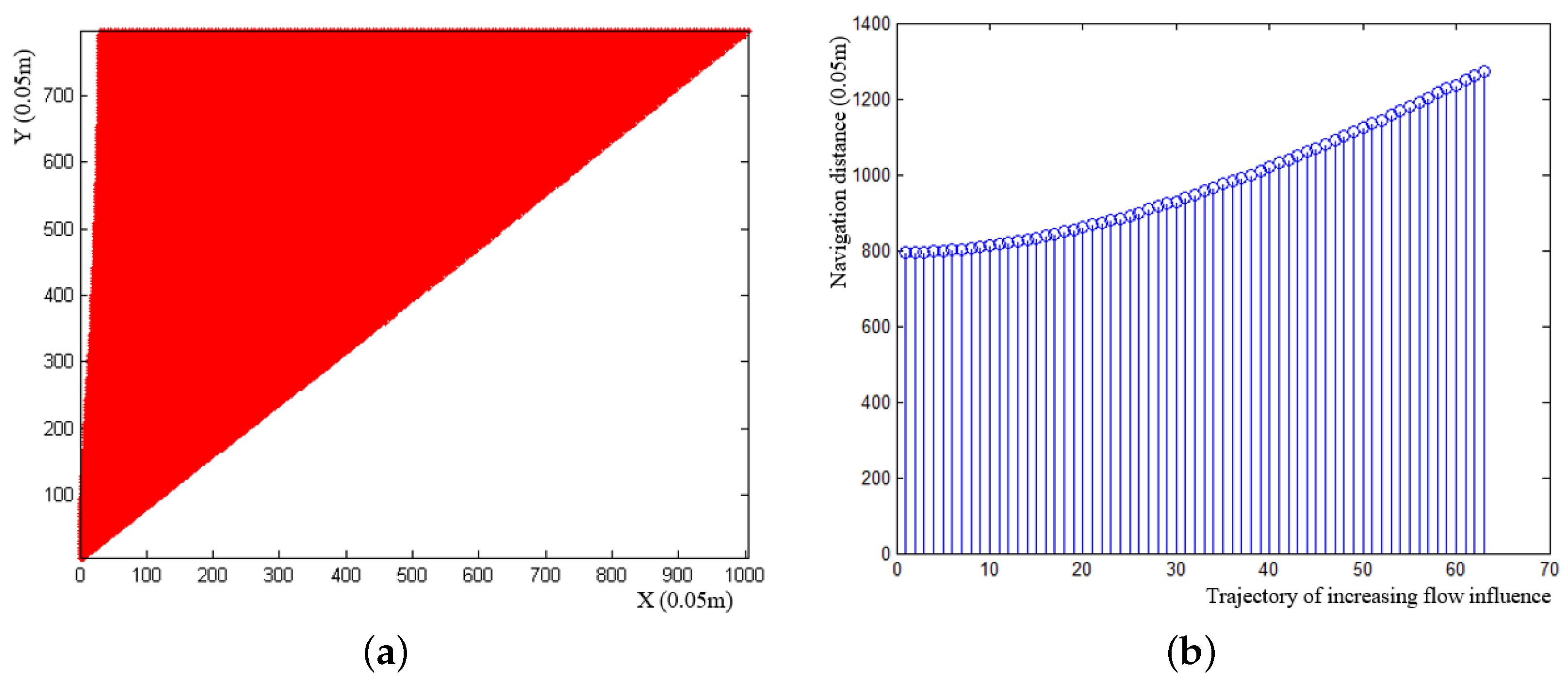
6.1.2. Analysis of Current Effects
In this section, the influence of the current is directly added to the navigation speed of the USV.
Figure 8a,b respectively show the change of the navigation path and the navigation path distance of the USV under the influence of a certain current velocity.
6.2. Search Algorithm Construction
In the process of constructing the algorithm, the wind and current effects are considered to be part of the path search generation value. Through experimental analysis, the influence of the wind on navigation presents a Gauss distribution, and the effect of the current is directly superimposed onto the speed of the USV.
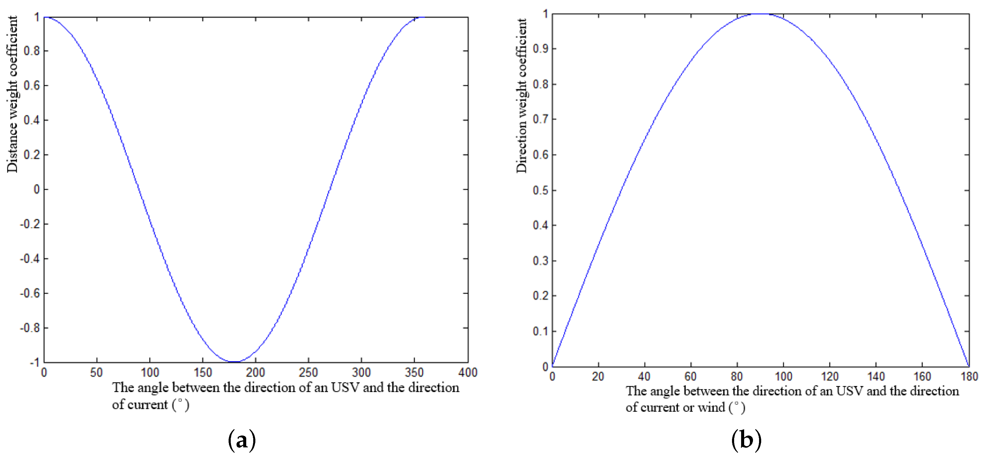
Figure 9a is a cos (x) figure. The
x-axis is the angle between the current direction and the direction of the USV, and the
y-axis is the weight of the search cost. According to the simulation results, with the change of the angle between the direction of the current and the course of the USV, the current velocity superimposed onto the velocity of the USV presents a cosine curve change.
Figure 9b is a figure of a sin (x) function from 0 to 180° (similar to other angles) on the basis of current impacts. The
x-axis represents the angle between the direction of the current or the wind and the course of the USV, and the
y-axis represents the weight of the search cost. When the current or wind is 90° to the heading, the weight value is the largest, that is, the cost of steering becomes higher; this can help a USV to avoid a position where its navigation course will be perpendicular to the direction of the current or the wind in the process of motion planning, and to avoid a situation where it will roll due to the disturbances of the current or the wind.
The A* search Algorithm 1 introduces the evaluation function F(x) when selecting the next exploration node of the current node:
represents the sum of the actual cost
from the starting point to the current point, and the evaluation cost
from the current point to the target point (as shown in Formula (
13). The weight of
is expressed as follows: distance cost + steering cost + time cost. The steering cost is proportional to the change of the rudder angle; the change of the USV speed presents the time cost, and the speed of the USV is affected by the wind and current; the distance cost principle is the shortest path principle, where the Euclidean distance is used for the heuristic distance calculation (as shown in Equation (
14)).
| Algorithm 1: Motion planning algorithm of a USV with the effects of wind and current. |
Input: map information, starting point, and end point. Output: USV rudder angles, navigation angles, path points (x, y). 1. Define the open list and close list, add the starting point to the open list and set it as the current point. 2. Move the current point to the close list and explore the F minimum around the current point. (1) If a point is already in the close list or cannot be passed, the point is ignored. (2) If the point is not in the open list, we add it to the open list and take the current point as the parent node of the point, and then record the F, G, and H values of the point. (3) If the point is already in the open list, the path is determined according to the G value, and the point with the lowest G value is the current point. 3. Under the influence of the wind and current environment, start to explore the appropriate trajectory based on the current node and the previous node, and then constantly adjust the rudder angle in the process of exploration. 4. The rudder angle adjustment range requires proper steering. (1) If the rudder angle at this time cannot meet the steering requirements in this environment, abandon the current node. Go to step 2 and select the sub-optimal node, and so on, until the node that meets the navigation requirements of the USV is found. (2) If the target point has already been added to the open list, then return to the starting point along with the parent node of each cell. 5. End (output planning information). |
7. Simulation Experiments and Analysis
7.1. Experimental Environments and Results
This section will introduce the environments and results of the experiments.
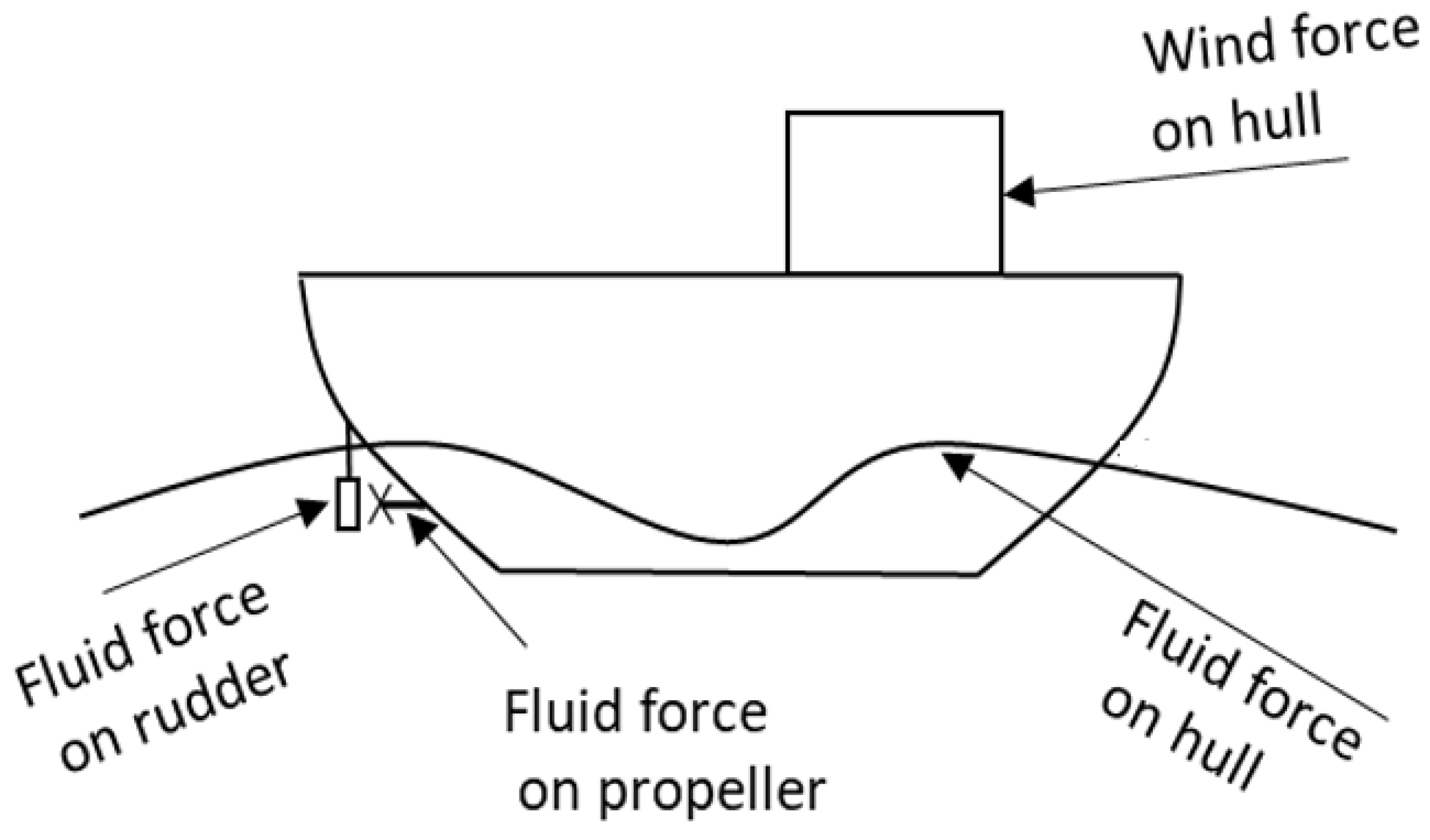
Figure 10 shows a schematic diagram of the force on the USV during navigation. Based on the dynamic model above, the corresponding motion model is established, and the corresponding trajectory cell is generated. In the experiment, the speed of the USV is 10 knots, the wind direction is 0°, the wind speed is 2 m/s, the current velocity in the
x-axis direction is 1 m/s, and the current velocity in the
y-axis direction is 1 m/s.
As shown in
Figure 11a, the starting point is (5, 24) and the ending point is (20, 10) in the environment without obstacles, and wind and current interfere with the USV motion planning experiment results (in the figure, the blue circle is the starting point, the green circle is the ending point, the green arrow represents current disturbances, and the red arrow represents wind disturbances). As shown in
Figure 11b, the starting point is (20, 10) and the ending point is (4, 26).
Figure 11c shows in detail the motion planning of the USV in the environment of the starting point (5, 24) and ending point (20, 5), without obstacles but with wind and current disturbances.
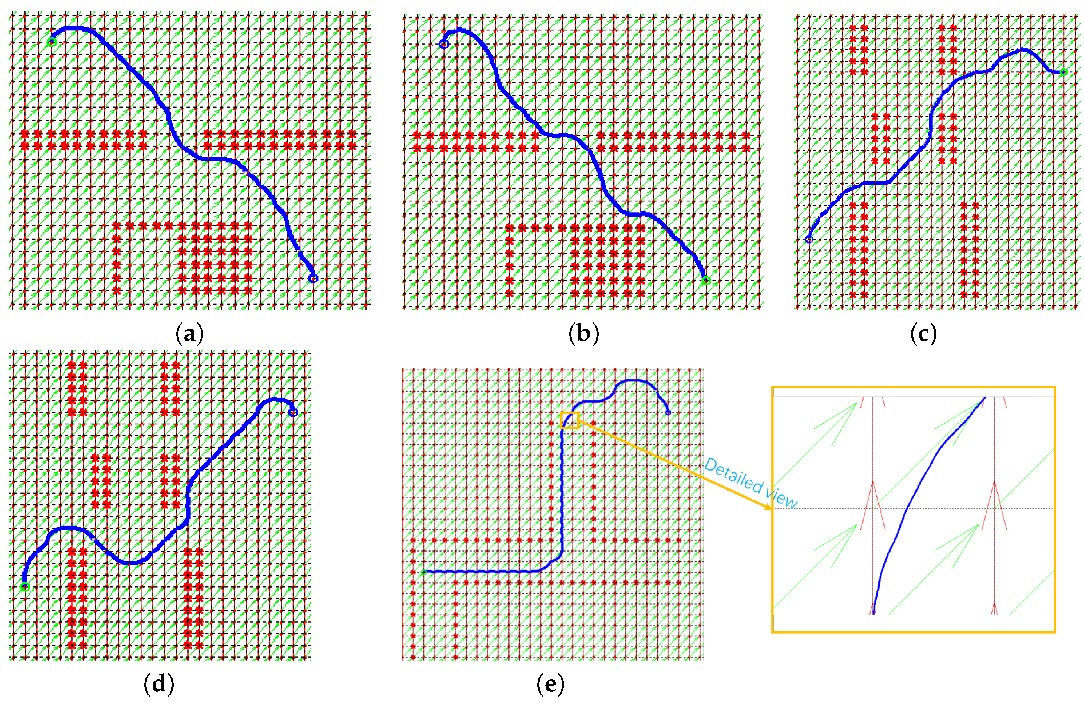
The experimental results of USV motion planning with obstacles and wind and current disturbances (the red asterisk is the obstacle) are shown in
Figure 12a. The starting point and ending point are (25, 6) and (5, 24), respectively. Note: We consider
Figure 11 and
Figure 12 as two-dimensional coordinate maps in which the unit of measurement used is meter.
The experimental results of the USV motion planning in the environment of the starting point (5, 24) and the ending point (25, 6) with obstacles and wind and current disturbances are shown in
Figure 12b. As shown in
Figure 12c, the starting point is (2, 9) and the ending point is (25, 24). The experimental results of USV motion planning in the environment of obstacles and wind and current disturbances are also shown in
Figure 12d. The experimental results of USV motion planning in the environment of the starting point (25, 24) and the ending point (2, 9) with obstacles and wind and current disturbances are shown in
Figure 12e, and the detail trajectory is shown in the right of
Figure 12e.
7.2. Analysis of Experimental Results
In the experiments, the characteristics of the USV dynamics and the influence of wind and current on the motion of a USV are fully considered. First, the disturbance effects of wind and current are simulated and analyzed, and the relevant characteristic parameters are extracted. Second, according to the influence of the wind and current, the regularization-trajectory cell is constructed to resist wind and current disturbances. Finally, a wind speed of 2 m/s and a current speed in the x-axis and y-axis directions of 1 m/s are simulated. The experiments show that the trajectory of the USV changes irregularly under the environment disturbances, but that the method proposed in this paper makes the trajectory as smooth as possible and achieves a short path planning with safety through the regularization-trajectory cell that allows it to resist the environment disturbances.
From the experiments, the highlights of our method are as follows: (1) On the basis of the regularization-trajectory cell, the smooth rudder command in the trajectory cell is considered; in the process of solving a motion planning problem, the short distance is taken as one of the optimization objectives. (2) Compared with the existing research (such as the method proposed in reference [
6]):
Our method takes into account the force process of the USV in real time by constructing the regularization-trajectory cell and carrying out motion planning according to the changes in force, while the method in reference [
6] solves the relevant problems by considering the influence of the current to realize path planning with a multi-objective optimisation method, there is no specific force analysis in the process of the navigation of the USV.
Our method can realize motion planning under more complex sea conditions by constructing the regularization-trajectory cell, which achieves practical and safe motion planning for a USV.
In this study, an objective function can be efficiently optimized, which can be easily implemented and may be widely used in the future.
8. Conclusions
In this paper, we tried to solve issues with the disturbances of wind and current on USV motion planning. From the perspectives of USV navigation characteristics, a motion planning method was proposed: first, existing problems were analyzed in detail, and the problem formulation was provided. Second, the USV’s dynamics model under the effects of wind and current was established. Third, the regularization-trajectory cell was constructed to provide reachable areas on the basis of a dynamics model. Furthermore, the USV’s motion state disturbed by wind and current effects was analyzed in detail. Based on the analysis, the rules and the regularization-trajectory cell were established. Finally, the regularization-trajectory cell, rules, and the A* algorithm were leveraged to construct the motion planning method for a USV under wind and current disturbances. The empirical results indicate the effectiveness of our proposed method that may help to achieve safe and efficient USV motion planning while considering the disturbances of wind and current; this is the key component in future attempts to overcome the influence of more complex environments.
In this study, the influence of waves was not considered, and the influence of waves may be more intense to some extent as compared to the influence of current and wind. Therefore, future research should consider the potential effects of waves more carefully. The problem may also be more complex; we have left this problem for future research.
Author Contributions
Methodology, S.G.; software, S.G.; validation, S.G.; formal analysis, S.G.; investigation, S.G.; resources, S.G.; data curation, S.G.; writing—original draft preparation, S.G.; writing—review and editing, C.Z.; visualization, S.G.; supervision, C.Z. and A.K.; project administration, C.Z., Y.W. and C.X.; funding acquisition, C.Z., Y.W. and C.X. All authors have read and agreed to the published version of the manuscript.
Funding
This work was supported by the National Science Foundation of China (NSFC) through Grant No. 52171349, the National Key R&D Program of China through Grant No. 2018YFC1407405, and the Zhejiang Provincial Science and Technology Program through Grant No. 2021C01010.
Institutional Review Board Statement
Not applicable.
Informed Consent Statement
Not applicable.
Data Availability Statement
The datasets generated during this study are available from the author, who can be reached by contacting
gshangd@163.com.
Conflicts of Interest
The authors declare no conflict of interest.
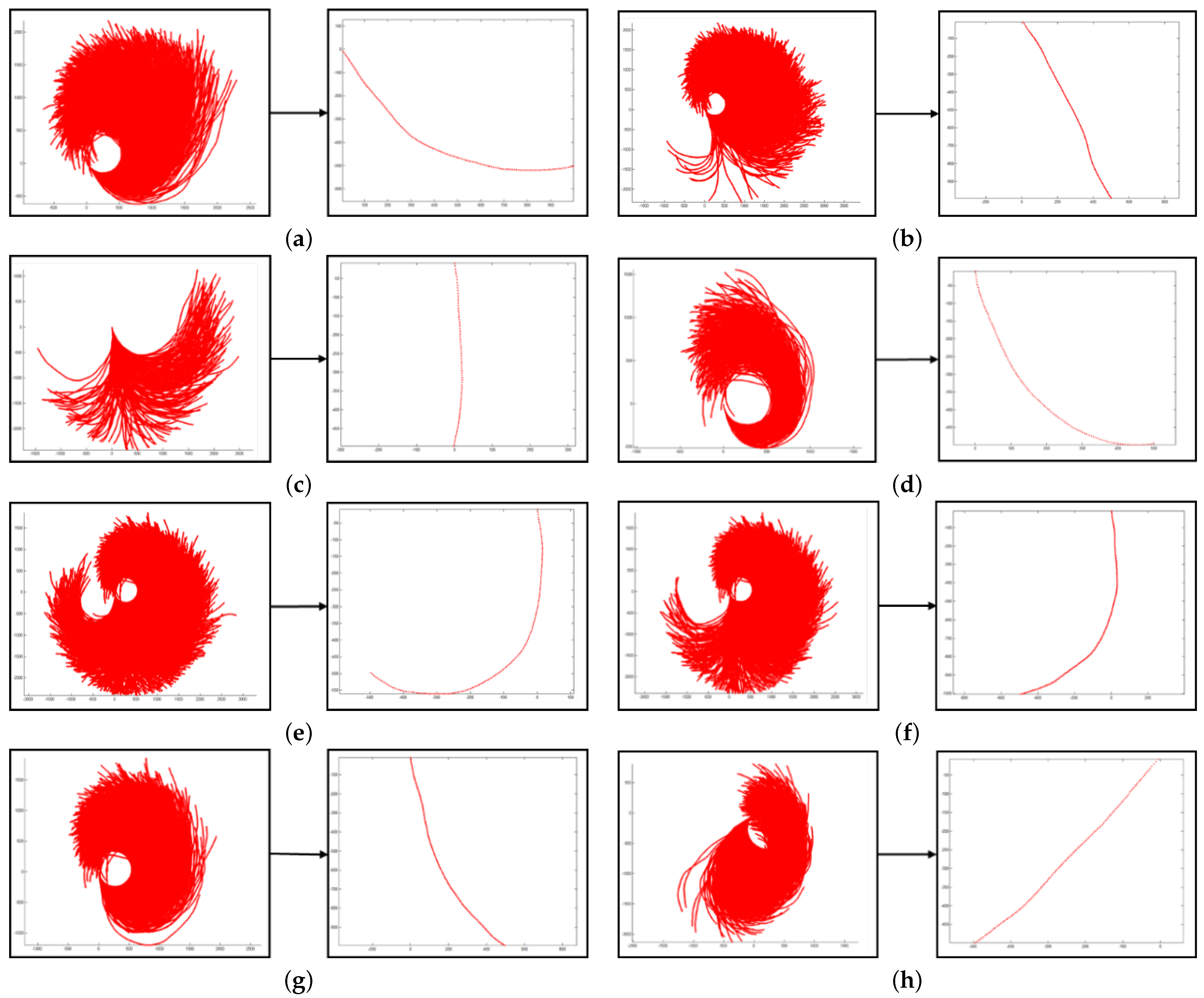
Appendix A. Regularization-TrajectoryCell Library
Figure A1.
Regularization-trajectory cell library: the first section. (a) Regularization-trajectory cells from the initial direction to 45° (rudder angle is 13.6°). (b) Time-varying trajectory cell from the initial direction to (rudder angle is −1.92°). (c) From the initial direction to the regularization-trajectory cell (rudder angle is −11.52°). (d) Time-varying trajectory cell from the initial direction to (rudder angle is −13.66°). (e) Time-varying trajectory cell from the initial direction to (rudder angle is 2.58°). (f) Time-varying trajectory cell from the initial direction to (rudder angle is −0.66°). (g) Time-varying trajectory cell from the initial direction to (rudder angle is −11.52°). (h) From the initial direction to the regularization-trajectory cell (rudder angle is −10.74°).
Figure A2.
Regularization-trajectory cell library: the second section. (a) Time-varying trajectory cell from the initial direction to (rudder angle is −5.32°). (b) Time-varying trajectory cell from the initial direction to (rudder angle is 3.8°). (c) From the initial direction to the time-varying track cell (rudder angle is −0.78°). (d) Time-varying trajectory cell from the initial direction to (rudder angle is −22.78°). (e) Time-varying trajectory cell from the initial direction to (rudder angle is 4.33°). (f) Time-varying trajectory cell from the initial direction to (rudder angle is −0.05°). (g) Time-varying trajectory cell from the initial direction to (rudder angle is −9.61°). (h) From the initial direction to the regularization-trajectory cell (rudder angle is −16.65°).
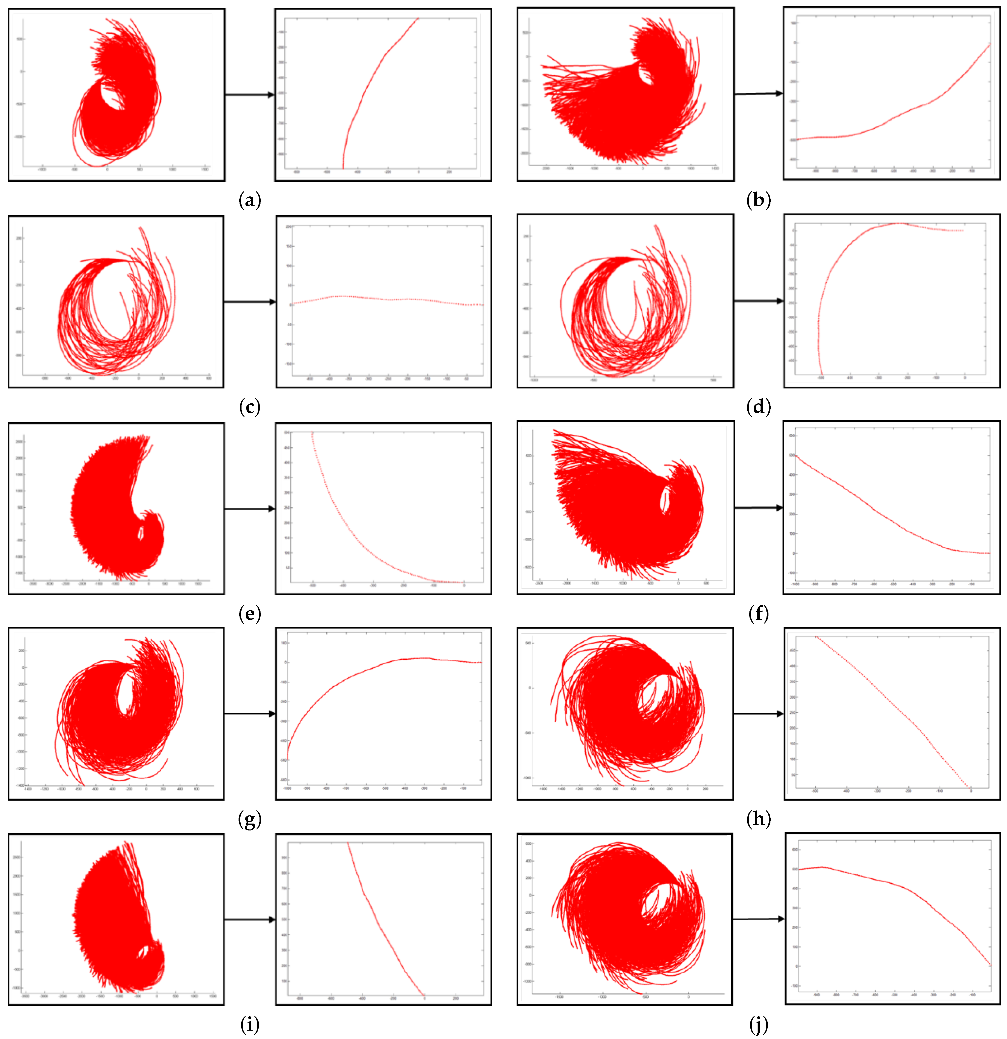
Figure A3.
Regularization-trajectory cell library: the third section. (a) Time-varying trajectory cell from the initial direction to (rudder angle is −25.79°). (b) Time-varying trajectory cell from the initial direction to (rudder angle is −9.74°). (c) From the initial direction to the regularization-trajectory cell (rudder angle is −34.68°). (d) Time-varying trajectory cell from the initial direction to (rudder angle is −34.64°). (e) Time-varying trajectory cell from the initial direction to (rudder angle is 0.84°). (f) Time-varying trajectory cell from the initial direction to (rudder angle is −13.68°). (g) From the initial direction to the regularization-trajectory cell (rudder angle is −29.17°). (h) From the initial direction to the regularization-trajectory cell (rudder angle is −29.96°). (i) Time-varying trajectory cell from the initial direction to (rudder angle is −8.25°). (j) Time-varying trajectory cell from the initial direction to (rudder angle is −27.19°).
![Jmse 10 00420 g0a3]()
References
- Liu, Y.; Bucknall, R. Path planning algorithm for unmanned surface vehicle formations in a practical maritime environment. Ocean Eng. 2015, 97, 126–144. [Google Scholar] [CrossRef]
- Gu, S.; Zhou, C.; Wen, Y.; Xiao, C.; Du, Z.; Huang, L. Path Search of Unmanned Surface Vehicle Based on Topological Location. Navig. China 2019, 42, 52–58. [Google Scholar]
- Zhou, C.; Huang, H.; Gu, S.; Chen, R.; Wen, Y.; Gan, L. Design and Implementation of Virtual Warning Buoy System for Over-Water Construction. Navig. China 2020, 43, 65–69. [Google Scholar]
- Zhou, C.; Gu, S.; Wen, Y.; Du, Z.; Xiao, C.; Huang, L.; Zhu, M. The review unmanned surface vehicle path planning: Based on multi-modality constraint. Ocean Eng. 2020, 200, 107043. [Google Scholar] [CrossRef]
- Singh, Y.; Sharma, S.; Sutton, R.; Hatton, D.; Khan, A. A constrained A* approach towards optimal path planning for an unmanned surface vehicle in a maritime environment containing dynamic obstacles and ocean currents. Ocean Eng. 2018, 169, 187–201. [Google Scholar] [CrossRef] [Green Version]
- Ma, Y.; Hu, M.; Yan, X. Multi-objective path planning for unmanned surface vehicle with currents effects. ISA Trans. 2018, 75, 137–156. [Google Scholar] [CrossRef] [PubMed]
- Thakur, A.; Svec, P.; Gupta, S.K. GPU based generation of state transition models using simulations for unmanned surface vehicle trajectory planning. Robot. Auton. Syst. 2012, 60, 1457–1471. [Google Scholar] [CrossRef] [Green Version]
- Song, R.; Liu, W.; Liu, Y.; Bucknall, R. A two-layered fast marching path planning algorithm for an unmanned surface vehicle operating in a dynamic environment. In Proceedings of the OCEANS 2015-Genova, Genova, Italy, 18–21 May 2015; pp. 1–8. [Google Scholar]
- Song, R.; Liu, Y.; Bucknall, R. A multi-layered fast marching method for unmanned surface vehicle path planning in a time-variant maritime environment. Ocean Eng. 2017, 129, 301–317. [Google Scholar] [CrossRef]
- Gal, O. Unified approach of unmanned surface vehicle navigation in presence of waves. J. Robot. 2011, 2011, 703959. [Google Scholar] [CrossRef] [Green Version]
- Niu, H.; Ji, Z.; Savvaris, A.; Tsourdos, A. Energy efficient path planning for Unmanned Surface Vehicle in spatially-temporally variant environment. Ocean Eng. 2020, 196, 106766. [Google Scholar] [CrossRef]
- Subramani, D.N.; Wei, Q.J.; Lermusiaux, P.F. Stochastic time-optimal path-planning in uncertain, strong, and dynamic flows. Comput. Methods Appl. Mech. Eng. 2018, 333, 218–237. [Google Scholar] [CrossRef]
- Wu, M.; Zhang, A.; Gao, M.; Zhang, J. Ship Motion Planning for MASS Based on a Multi-Objective Optimization HA* Algorithm in Complex Navigation Conditions. J. Mar. Sci. Eng. 2021, 9, 1126. [Google Scholar] [CrossRef]
- Hart, P.E.; Nilsson, N.J.; Raphael, B. A formal basis for the heuristic determination of minimum cost paths. IEEE Trans. Syst. Sci. Cybern. 1968, 4, 100–107. [Google Scholar] [CrossRef]
- Goh, C.K.; Tan, K.C.; Liu, D.; Chiam, S.C. A competitive and cooperative co-evolutionary approach to multi-objective particle swarm optimization algorithm design. Eur. J. Oper. Res. 2010, 202, 42–54. [Google Scholar] [CrossRef]
- Alvarez, A.; Caiti, A.; Onken, R. Evolutionary path planning for autonomous underwater vehicles in a variable ocean. IEEE J. Ocean. Eng. 2004, 29, 418–429. [Google Scholar] [CrossRef]
- Eichhorn, M. Optimal routing strategies for autonomous underwater vehicles in time-varying environment. Robot. Auton. Syst. 2015, 67, 33–43. [Google Scholar] [CrossRef]
- Wang, L. Trajectory Planning and Path Following Techniques of Unmanned Surface Vehicle. Ph.D. Thesis, Harbin Engineering University, Harbin, China, 2016. [Google Scholar]
- Sethian, J.A. Level Set Methods and Fast Marching Methods: Evolving Interfaces in Computational Geometry, Fluid Mechanics, Computer Vision, and Materials Science; Cambridge University Press: Cambridge, UK, 1999; Volume 3. [Google Scholar]
- Tsitsiklis, J.N. Efficient algorithms for globally optimal trajectories. IEEE Trans. Autom. Control 1995, 40, 1528–1538. [Google Scholar] [CrossRef] [Green Version]
- Poonganam, S.N.J.; Gopalakrishnan, B.; Avula, V.S.S.B.K.; Singh, A.K.; Krishna, K.M.; Manocha, D. Reactive navigation under non-parametric uncertainty through hilbert space embedding of probabilistic velocity obstacles. IEEE Robot. Autom. Lett. 2020, 5, 2690–2697. [Google Scholar] [CrossRef]
- Du, Z.; Wen, Y.; Xiao, C.; Zhang, F.; Huang, L.; Zhou, C. Motion planning for unmanned surface vehicle based on trajectory unit. Ocean Eng. 2018, 151, 46–56. [Google Scholar] [CrossRef]
- Du, Z.; Wen, Y.; Xiao, C.; Huang, L.; Zhou, C.; Zhang, F. Trajectory-cell based method for the unmanned surface vehicle motion planning. Appl. Ocean. Res. 2019, 86, 207–221. [Google Scholar] [CrossRef]
- Ogawa, O. MMG report I: Mathematical model of control movement. Jpn. Shipbuild. Soc. 1977. [Google Scholar]
- Zhu, M.; Xiao, C.; Gu, S.; Du, Z.; Wen, Y. A Circle Grid-based Approach for Obstacle Avoidance Motion Planning of Unmanned Surface Vehicles. arXiv 2022, arXiv:2202.04494. [Google Scholar]
- Tian, C. Numerical Simulation of Ship’s Maneuvering Motion in the Wind, Wave and Current. Master’s Thesis, Wuhan University of Technology, Wuhan, China, 2003. [Google Scholar]
- Shi, C. Study on Simulation Mathematical Model of Ship Maneuvering Motion in Wind and Wave. Master’s Thesis, Harbin Engineering University, Harbin, China, 2011. [Google Scholar]
- Jia, X.; Yang, Y. Mathematical Model of Ship Motion-Mechanism Modeling and Identification Modeling; Publishing House of Dalian Maritime University: Dalian, China, 1999. [Google Scholar]
- Zhou, C.; Gu, S.; Wen, Y.; Du, Z.; Xiao, C.; Huang, L.; Zhu, M. Motion planning for an unmanned surface vehicle based on topological position maps. Ocean Eng. 2020, 198, 106798. [Google Scholar] [CrossRef]
- Gu, S.; Zhou, C.; Wen, Y.; Zhong, X.; Zhu, M.; Xiao, C.; Du, Z. A motion planning method for unmanned surface vehicle in restricted waters. Proc. Inst. Mech. Eng. Part M J. Eng. Marit. Environ. 2020, 234, 332–345. [Google Scholar] [CrossRef]
Figure 1.
Motion planning algorithm without considering wind and current disturbances.
Figure 1.
Motion planning algorithm without considering wind and current disturbances.
Figure 2.
Structure of the motion planning method for USVs based on the regularization-trajectory cell.
Figure 2.
Structure of the motion planning method for USVs based on the regularization-trajectory cell.
Figure 3.
USV turning experiments. (a) Turning experiment of a USV without environmental disturbances. (b) Turning experiment of a USV with current disturbances. (c) Turning experiment of a USV with wind disturbances. (d) Turning experiment of a USV with current and wind disturbances.
Figure 3.
USV turning experiments. (a) Turning experiment of a USV without environmental disturbances. (b) Turning experiment of a USV with current disturbances. (c) Turning experiment of a USV with wind disturbances. (d) Turning experiment of a USV with current and wind disturbances.
Figure 4.
Reachable points of the rudder angle at 15°; the heading is explored at 0.5° intervals.
Figure 4.
Reachable points of the rudder angle at 15°; the heading is explored at 0.5° intervals.
Figure 5.
Construction process of a regularization-trajectory cell.
Figure 5.
Construction process of a regularization-trajectory cell.
Figure 6.
Schematic diagram of ship motion under the influence of wind and current.
Figure 6.
Schematic diagram of ship motion under the influence of wind and current.
Figure 7.
Wind impacts from 0 to 8 m/s. (a) Trajectories under wind disturbances from 0 to 8 m/s. (b) Heading statistics of wind impacts from 0 to 8 m/s. (c) Distance statistics of wind impacts from 0 to 8 m/s.
Figure 7.
Wind impacts from 0 to 8 m/s. (a) Trajectories under wind disturbances from 0 to 8 m/s. (b) Heading statistics of wind impacts from 0 to 8 m/s. (c) Distance statistics of wind impacts from 0 to 8 m/s.
Figure 8.
Current impacts at from 0 to 11.3 m/s. (a) Trajectory diagram under the current disturbances from 0 to 11.3 m/s. (b) Trajectory distance statistics under the current disturbances from 0 to 11.3 m/s.
Figure 8.
Current impacts at from 0 to 11.3 m/s. (a) Trajectory diagram under the current disturbances from 0 to 11.3 m/s. (b) Trajectory distance statistics under the current disturbances from 0 to 11.3 m/s.
Figure 9.
Wind and current impacts on the weight of motion planning. (a) Current impacts on the weight of motion planning. (b) Wind and current impacts on the planned heading of motion.
Figure 9.
Wind and current impacts on the weight of motion planning. (a) Current impacts on the weight of motion planning. (b) Wind and current impacts on the planned heading of motion.
Figure 10.
Force diagram of the USV during navigation.
Figure 10.
Force diagram of the USV during navigation.
Figure 11.
Motion planning for a USV in a free open-sea environment at different starting and ending points, considering wind and current disturbances. (a) Motion planning for a USV at the starting point (5, 24) and the ending point (20, 10). (b) Motion planning for a USV at the starting point (20, 10) and the ending point (4, 26). (c) Local details of USV motion planning at the starting point (5, 24) and the ending point (20, 5).
Figure 12.
Motion planning for a USV in obstacle environments at different starting and ending points, considering wind and current disturbances. (a) Motion planning for a USV at the starting point (25, 6) and the ending point (5, 24). (b) Motion planning for a USV at the starting point (5, 24) and the ending point (25, 6). (c) Motion planning for a USV at the starting point (2, 9) and the ending point (25, 24). (d) Motion planning for a USV at the starting point (25, 24) and the ending point (2, 9). (e) Motion planning for a USV at the starting point (25, 24) and the ending point (2, 9).
| Publisher’s Note: MDPI stays neutral with regard to jurisdictional claims in published maps and institutional affiliations. |
© 2022 by the authors. Licensee MDPI, Basel, Switzerland. This article is an open access article distributed under the terms and conditions of the Creative Commons Attribution (CC BY) license (https://creativecommons.org/licenses/by/4.0/).


