Ship Traffic Flow Prediction in Wind Farms Water Area Based on Spatiotemporal Dependence

Abstract

To analyze the changing characteristics of ship traffic flow in wind farms water area, and to improve the accuracy of ship traffic flow prediction, a Gated Recurrent Unit (GRU) of a Recurrent Neural Network (RNN) was established to analyze multiple traffic flow sections in complex waters based on their traffic flow structure. Herein, we construct a spatiotemporal dependence feature matrix to predict ship traffic flow instead of the traditional ship traffic flow time series as the input of the neural network. The model was used to predict the ship traffic flow in the water area of wind farms in Yancheng city, Jiangsu Province. Autoregressive Integrated Moving Average (ARIMA), Support-Vector Machine (SVM) and Long Short-Term Memory (LSTM) were chosen as the control tests. The GRU method based on the spatiotemporal dependence is more accurate than the current mainstream ship traffic flow prediction methods. The results verify the reliability and validity of the GRU method.

1. Introduction

Marine wind energy is a green renewable resource that has the advantages of cleanliness, low development cost, and abundant reserves [1,2]. The development of marine wind energy under the background of encouraging sustainable economic development is conducive to alleviating the energy crisis and preventing climate change. With the development of offshore wind power technology, offshore wind farm construction has gradually become a key development field [3]. However, the offshore wind farm needs to occupy a large area of water in the process of construction, and some ship traffic inevitably flows through the wind farm. With the increasing frequency of offshore wind power construction, the risk assessment of ship navigation in wind farms water area has also attracted the attention of scholars at home and abroad [4].

In the water area of the wind farm, ships need to be in close contact with the wind turbine, and the working frequency is very high. Compared with ships in other water areas, the collision probability of ships in the water area of a wind farm is greater [5,6]. Especially in severe weather—such as strong winds, large waves, and dense fog—the maneuverability of the ship is limited, the visibility in the water area is reduced, and the risk of collision between the ships and the wind turbines is further exacerbated [7]. With the increase in offshore wind power construction, the safety of ship navigation in the waters of offshore wind farms has gradually attracted the extensive attention of relevant scholars. At present, the research on ship navigation safety in the water area of wind farms mainly focuses on exploring the variation law of collision risk between ships and offshore wind turbines [8,9].

However, the impact of wind farm characteristics and ship traffic flow characteristics is not fully considered, and the established collision risk model often cannot reflect the actual situation of ship/wind turbine collisions. Therefore, it is necessary to analyze the ship traffic flow in the wind farms water area as the basis of ship navigation risk assessment [10,11]. By analyzing the variation in characteristics of ship traffic flow, mining the potential regularity of traffic flow data, and predicting the traffic flow state in the future, we can provide a theoretical basis for the formulation of traffic control measures in the wind farms water area.

Therefore, we propose a method to predict the traffic volume in wind farm areas based on spatiotemporal dependence. A feature matrix is constructed to represent the spatial relationship of traffic flow based on Pearson’s Correlation Coefficient (PCC), and then GRU is established to predict the ship traffic flow. The construction in this paper has two folders: Firstly, the spatial effects of traffic flow on different routes are considered. Secondly, the matrix is used as the input of the neural network instead of a single value. The method proposed in this paper can support the construction of safety supervision in wind farms water area.

The remainder of this paper is organized as follows: Section 2 reviews research related to the research and safety of wind farm water and traffic flow prediction. Section 3 elaborates on the framework construction and methodological development, followed by case studies in Section 4. Finally, Section 5 discusses the major findings and potential research improvements, and conclusions are summarized in Section 5

2. Literature Review

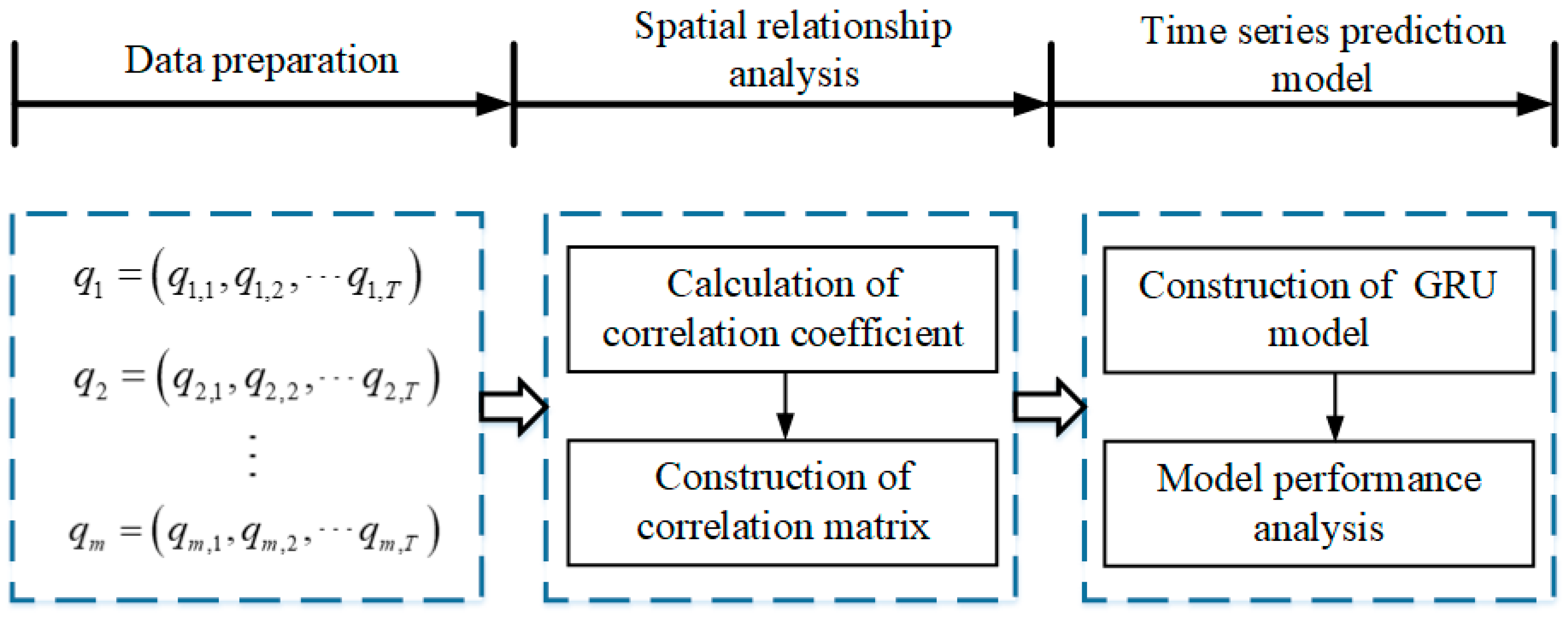
Traffic flow prediction is an important topic in maritime traffic research. Recently, the study of ship traffic flow prediction can be divided into statistical methods and data-driven methods.

Several statistical models have been applied extensively in traffic flow prediction, including linear regression, ARIMA, Kalman filtering, Bayesian networks, Markov models, etc. Sun et al. (2003) introduced local linear regression into traffic flow prediction research [12]. Williams and Hoel (2003) adopted the seasonal ARIMA process to forecast vehicular traffic flow [13]. Getahun (2021) modeled a time series of road traffic accidents based on ARIMA [14]. Guo et al. (2014) developed an adaptive Kalman filter method for stochastic traffic flow rate prediction [15], while Xie et al. (2007) researched traffic flow prediction using a Kalman filter with discrete wavelet decomposition [16]. Saeedmanesh et al. (2021) developed an extended Kalman filter approach for real-time state estimation in multiregion MFD urban networks [17]. Smith et al. (1997, 2002) proposed a nonparametric method for traffic flow forecasting, and compared parametric and nonparametric models [18,19]. Zheng and Su (2014) researched traffic flow forecasting using a constrained linearly sewing principal component algorithm [20]. Wang et al. (2021) proposed a non-parametric model with an optimized training strategy for vehicle traffic flow prediction [21]. Castillo et al. (2008) introduced a Bayesian network for traffic flow prediction [22]. Wang et al. (2014) designed an architecture for traffic flow prediction using a new Bayesian combination method [23]. Afrin et al. (2021) estimated traffic congestion based on a Bayesian network [24]. Qi and Ishak (2014) developed a hidden Markov model for the prediction of traffic flow on freeways [25]. Rajawat et al. (2021) developed a comprehensive framework for the prediction of human mobility patterns based on a hidden Markov model [26].

In recent years, data-driven methods have been widely used in traffic flow prediction. The advantage of these methods is their ability to predict future traffic flow directly from the given big data without modeling the traffic flow phenomenon. Many researchers have applied SVM regression models to traffic flow prediction and achieved good results [27,28,29]. Some improved SVM methods are also widely used [30,31]. Yao et al. (2014) developed a framework in multistep-ahead prediction for rock displacement surrounding a tunnel, using an improved SVM [32]. Toan et al. (2021) applied an SVM for short-term traffic flow prediction [33].

Another widely used method is the K-nearest neighbor model, which is easy to implement because the processes of training data and estimating parameters are simple. Hong et al. (2015) developed a hybrid multimetric K-nearest neighbor regression model for traffic flow prediction [34]. Akbari et al. (2011) applied the K-nearest neighbor algorithm for daily inflow forecasting [35]. Yu et al. (2016) designed a prediction model for multiple-timestep prediction of traffic conditions [36]. Another very important method is machine learning. Many kinds of research for traffic prediction based on machine learning have been published [37,38,39,40,41,42]. Li (2016) applied dynamic fuzzy neural networks for traffic flow prediction [43]. Huang et al. (2014) proposed a Deep Belief Network (DBN) for traffic flow prediction, which is a deep architecture [44]. Yang et al. (2016) designed a type of unsupervised learning architecture of the neural network approach for traffic flow prediction using the Taguchi method [45]. Lu et al. (2021) proposed a combined method for short-term traffic flow prediction based on a recurrent neural network [46].

In summary, many researchers have made great progress in the research of traffic flow prediction, but the assumption that the model parameterization performs relatively badly in variable traffic conditions affects the majority of statistical models. On the other hand, data-driven models such as deep learning techniques are often used to make predictions. Although the accuracy of the deep learning method is higher than that of other algorithms, the training time is much longer than that of other algorithms. The GRU has fewer parameters than other models, reducing the risk of overfitting, and has a shorter training time. Additionally, the GRU can simultaneously consider the influence of features and historical time series. At present, GRU networks are mainly used in classification, regression, and time-series prediction problems. Therefore, a GRU was established to predict the ship traffic flow in this research.

Several studies have emerged over recent years covering many aspects of wind farms, such as site selection [47,48], operation and maintenance [49,50,51], and wildlife impact [52,53], among others. However, research on traffic flow prediction in the water area of wind farms is rare at present, and most such studies take a single port or channel section as their research object, not considering the spatiotemporal dependence of ship traffic flow. Therefore, taking the supervision of maritime traffic safety in complex waters as the starting point, the water area of Yancheng wind farms was selected as the research object to predict ship traffic flow in different routes in the water area of the wind farms.

3. Methodology

The logical framework for the prediction of ship traffic flow in wind farm waters is depicted in Figure 1; it consists of three components: data preparation, spatial relationship analysis, and time-series prediction model.

3.1. Data Preparation

As of December 2004, the International Maritime Organization (IMO) required all vessels over 299 GT to install an Automatic Identification System (AIS) transponder on board [54]. The increasing number of ships equipped with AISs provides a lot of basic data for traffic flow prediction research. AIS data are received as a series of messages following a nonstandard pattern of irregular time intervals. Since there is a lot of noise in the raw AIS data, it is necessary to preprocess the data. Firstly, the data of ship position abnormality, speed abnormality, and course abnormality in the experimental dataset are removed based on the algorithm proposed by [55]. Then, the linear interpolation method should be used to interpolate the ship’s AIS data per 10 seconds.

3.2. Analysis of Spatial Dependence of Ship Traffic Flow

For complex waters, such as wind farms water areas, the ship traffic flow may be affected by the traffic conditions of adjacent routes. Therefore, considering the spatial ship traffic flow dependence, Pearson’s Correlation Coefficient (PCC) method was used to calculate the correlation coefficient between the traffic flows of adjacent routes [56,57]. PCC is the covariance of the two variables divided by the product of their standard deviations.

Adding the route information with high correlation to the prediction model improves the accuracy of the marine traffic flow prediction model. If the traffic flow sequence of section x and section y is as follows:

$$q_x=\left(q_{x,1},q_{x,2},\cdots q_{x,T}\right),$$

(1)

$$q_y=\left(q_{y,1},q_{y,2},\cdots q_{y,T}\right),$$

(2)

then the correlation coefficient of the two sections is given by:

$${\rho }_{x,y}=\frac{{\displaystyle {\sum }_{i=1}^T(q_{x,i}-\overline{q_x})}(q_{y,i}-\overline{q_y})}{\sqrt{{{\displaystyle {\sum }_{i=1}^T(q_{y,i}-\overline{q_y})}}^2}\sqrt{{{\displaystyle {\sum }_{i=1}^T(q_{y,i}-\overline{q_y})}}^2}},$$

(3)

where ρ_x,y is the degree of correction between x and y, referred to as the correlation coefficient, while T represents the length of the time series. The closer ρ_x,y is to 1, the greater the correlation between the target section and the adjacent section. When ρ_x,y = 0, there is no correlation between the target section and adjacent sections. When 0 < ρ_x,y < 0.5, this indicates that the correlation between the target section and adjacent sections is low. To ensure the prediction accuracy of the model, 0.5 ≤ ρ_x,y < 1 was set as the spatial threshold range.

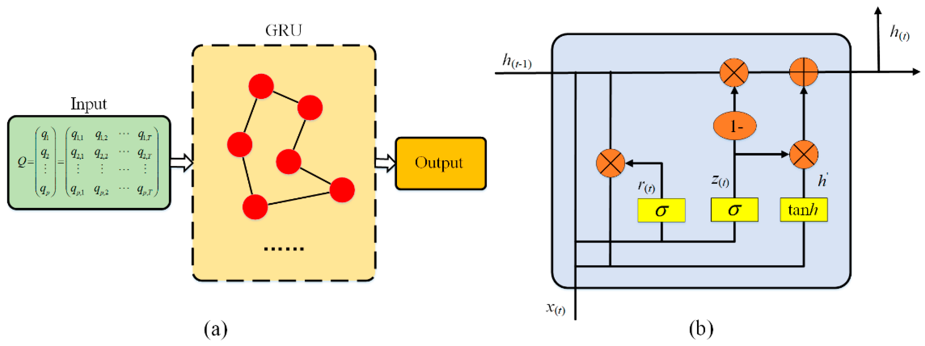
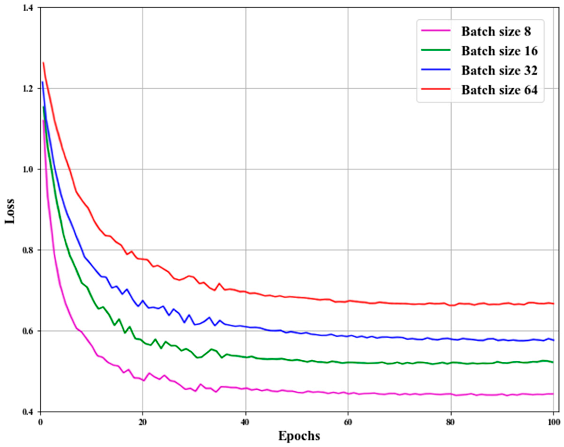
3.3. Time-Series Prediction Model Based on an Improved Recurrent Neural Network

A GRU can be used to mine the time characteristics of traffic flow and capture the time dependence of ship traffic flow [58,59,60]. Cho et al. introduced a GRU as a gating mechanism in recurrent neural networks [61]. The GRU’s functions are similar to those of a Long Short-Term Memory (LSTM) network with a forget gate, but with fewer parameters. The GRU outperformed LSTM on certain tasks, such as polyphonic music modeling, speech signal modeling, and natural language processing. The GRU also uses only two parameters, which can help to reduce the risk of overfitting. The basic structure of the GRU is shown in Figure 2.

x_(t) represents the input signal vector of the current node; h_{(t − 1)} represents the hidden state vector passed down from the previous node, h_(t) is the output vector, and $h_{(t)}^{\prime }$ is candidate activation vector; r_(t) is the reset gate vector, z_(t) is the update gate vector, while $\sigma$ represents the original function, and is a sigmoid function. The GRU uses x_(t) and h_{(t − 1)} to obtain two gating states; the functions of the reset gate and update gate are as follows:

$$r_{(t)}=\mathrm{Sigmoid}\_1(W_r(h_{(t-1)},x_{(t)})),$$

(4)

$$z_{(t)}=\mathrm{Sigmoid}\_2(W_z(h_{(t-1)},x_{(t)})),$$

(5)

where W_r is the weight matrix of reset gate, while W_z is the weight matrix of the update gate. After obtaining the gating signal, use $h_{(t-1)}^{\prime }=r_{(t)}\odot h_{(t-1)}$ to reset the data, then splice $h_{(t-1)}^{\prime }$ and x_(t). The activation function tanh is used to standardize the data to obtain $h_{(t)}^{\prime }$; the calculation formula is as follows:

$$h_{(t)}^{\prime }=\tan \mathrm{h}\left(W_{h^{\prime }}\left(h_{(t-1)}\odot r_{(t)},x_{(t)}\right)\right),$$

(6)

where the operator $\odot$ denotes the Hadamard product, $W_{h^{\prime }}$ is the weight matrix of candidate activation in the GRU, and $h_{(t)}^{\prime }$ mainly contains the current input x_(t), which adds $h_{(t)}^{\prime }$ to the current hidden state and effectively remembers the current state.

In the last memory update stage, forgetting and memorizing steps are both used, as is the previously obtained update gate z; the update expression is as follows:

$$h_{(t)}=z_{(t)}\odot h_{(t-1)}+(1-z_{(t)})\odot h_{(t)}^{\prime },$$

(7)

where $h_{(t)}^{}$ represents the output of the network at the moment t and $z_{(t)}\in \left(0,1\right)$. The input of each layer of the GRU considers the output of the previous layer of the GRU, so as to capture the timing relationship of ship traffic flow. After constructing a GRU, it is used as the basic unit from sequence to sequence as a model to generate the final prediction result.

The ship traffic flow in an area is related not only to the actual traffic flow in the given moments, but also to the spatially related route. Therefore, compared with the traditional ship traffic flow prediction method, a PCC algorithm can be introduced to calculate the correlation of traffic flow between different routes. This method can screen the areas with high correlation and reconstruct the spatiotemporal dependence matrix, in order to improve the input of the GRU model and to predict the ship traffic flow in complex waters more accurately. The algorithm flow is as follows:

(1) According to the characteristics of traffic flow structure in complex waters, the temporal and spatial characteristic matrix of multiple observation sections is defined as Q.

$$Q=\left(\begin{array}{c}{q}_1\\ q_2\\ ⋮\\ q_m\end{array}\right)=\left(\begin{array}{cccc}{q}_{1,1}& q_{1,2}& \cdots & q_{1,T}\\ q_{2,1}& q_{2,2}& \cdots & q_{2,T}\\ ⋮& ⋮& \cdots & ⋮\\ q_{m,1}& q_{m,2}& \cdots & q_{m,T}\end{array}\right),$$

(8)

where q_m is the time series of the observation section, and $q_{m,T}$ is the traffic volume of observation section m at the moment T;

(2) Calculate the correlation coefficient between the traffic flow at the observation section of two routes, constructing a spatial correlation matrix as follows:

$${\rho }_{xy}=\left(\begin{array}{cccc}{\rho }_{1,1}& {\rho }_{1,2}& \cdots & {\rho }_{1,m}\\ {\rho }_{2,1}& {\rho }_{2,2}& \cdots & {\rho }_{2,m}\\ ⋮& ⋮& \cdots & ⋮\\ {\rho }_{m,1}& {\rho }_{m,2}& \cdots & {\rho }_{m,m}\end{array}\right);$$

(9)

(3) Rank traffic flow correlation between sections. Select the sections to be predicted and sort the other sections by correlation;

(4) Set the correlation threshold $\delta$. The sections with a correlation greater than $\delta$ are reconstructed into a new spatiotemporally dependent characteristic matrix;

(5) Build the GRU model. The input of the GRU model is improved by using the reconstructed spatiotemporal dependence characteristic matrix, and the improved GRU is used to predict ship traffic flow;

(6) Calculate the Mean Absolute Percentage Error (MAPE); taking the minimum MAPE as the final optimization goal of the model, the optimal spatial threshold is determined;

(7) Results and analysis: To quantitatively analyze the prediction results and the performance of the model, the Mean Absolute Error (MAE), Root-Mean-Square Error (RMSE), Mean Absolute Percentage Error (MAPE), and R² are used as prediction and evaluation indicators. The calculation method is as follows:

$$\mathrm{MAE}=\frac{1}{n}{\displaystyle {\sum }_1^n\left|p_i-x_i\right|},$$

(10)

$$\mathrm{RMSE}=\sqrt{\frac{1}{n}{\displaystyle {\sum }_1^n{(p_i-x_i)}^2}},$$

(11)

$$\mathrm{MAPE}=\frac{1}{n}{\displaystyle {\sum }_1^n\frac{\left|p_i-x_i\right|}{x_i}}\times 100,$$

(12)

$${\mathrm{R}}^2=1-\frac{{\displaystyle {\sum }_1^n{(p_i-x_i)}^2}}{{\displaystyle {\sum }_1^n{(\overline{x_i}-x_i)}^2}},$$

(13)

where p_i is the predicted value obtained by PCC–GRU and by SVM, LSTM, and ARIMA in the control experiment; x_i is the actual value; $\overline{x_i}$ is the average of the actual flow section values.

4. Case Study

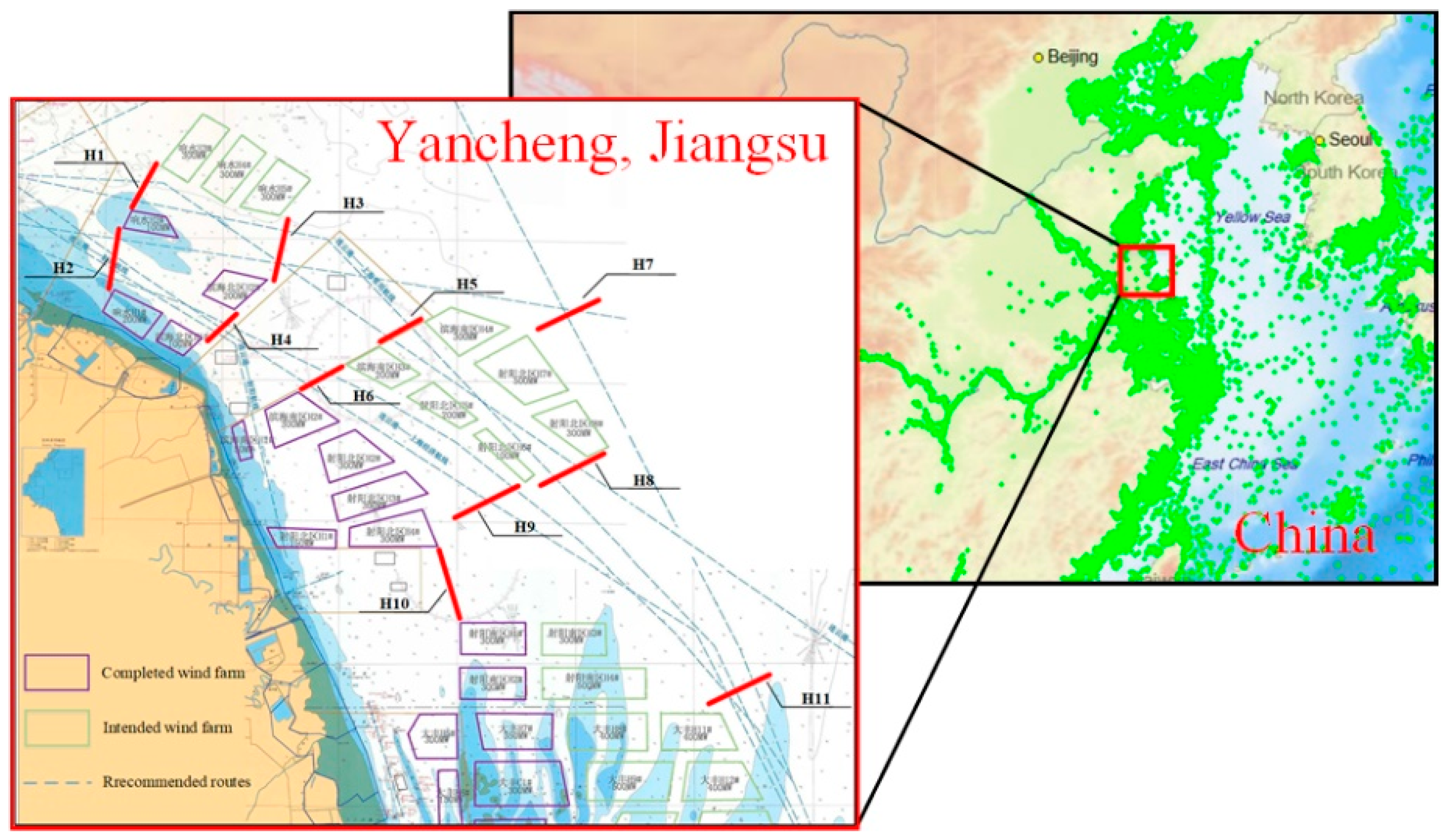
4.1. Research Area and Data

Due to the influence of meteorological and hydrological conditions, construction conditions, and water area location, the water area traffic environment of wind farms presents complex temporal and spatial characteristics. Based on AIS data, real-time prediction of ship traffic flow changes in different stages of wind farm groups can provide an effective means for daily maintenance of wind farms and safety monitoring in the process of construction.

To verify the effectiveness and feasibility of the model, the wind farm water area in Jiangsu Province was selected as the research object, as shown in Figure 3. The cross-section flow statistics of complex routes in the region were evaluated. The routes observed in this research were routes recommended in nautical charts, and the observation section was set in these routes. If a ship passes through the observation section, the traffic volume increases by 1.

The cross-sectional diagram is shown in Figure 3. The location information of the section is shown in

Table 1. Coordinates of the observation section.

Sections	P1	P2
H1	120.06495° E 34.75165° N	120.13086° E 34.96235° N
H2	120.02375° E 34.69723° N	119.96195° E 34.42275° N
H3	120.35502° E 34.76512° N	120.27413° E 34.64402° N
H4	120.26468° E 34.49281° N	120.20728° E 34.42028° N
H5	120.57021° E 34.48273° N	120.47371° E 34.43313° N
H6	120.47302° E 34.35673° N	120.57023° E 34.30368° N
H7	121.30618° E 34.65731° N	121.08612° E 34.45872° N
H8	121.04723° E 34.20372° N	120.93305° E 34.15846° N
H9	120.88817° E 34.13275° N	120.77619° E 34.08367° N
H10	120.72357° E 34.06888° N	120.78652° E 33.81706° N
H11	121.32603° E 33.78164° N	121.21804° E 33.26723° N

. The traffic flow time series from 1 to 29 March 2021 was selected as the training data, and the traffic flow data on 30 March were used as the verification set. The ship traffic flow data of sections H1–H11 were collected in hours, and the ship traffic flow data for one day were obtained, as shown in

Table 2. Ship traffic flow per hour on 30 March 2021.

Time	q1	q2	q3	q4	q5	q6	q7	q8	q9	q10	q11
0:00	2	2	3	3	2	2	5	5	1	3	5
1:00	2	1	2	4	6	3	4	3	3	3	10
2:00	5	3	4	3	4	4	3	2	2	3	6
3:00	2	3	6	4	5	3	4	5	6	3	6
4:00	4	4	8	4	7	6	6	2	7	6	9
5:00	4	5	5	2	6	3	2	4	4	3	6
6:00	5	2	6	5	9	4	3	6	2	5	11
7:00	5	3	3	2	3	5	4	5	3	2	4
8:00	7	4	4	4	4	5	2	5	3	5	5
9:00	5	2	3	3	4	4	5	7	8	6	2
10:00	4	5	3	4	6	3	3	5	2	5	9
11:00	6	4	2	3	7	4	5	4	4	3	13
12:00	7	2	7	5	2	2	1	7	6	4	6
13:00	6	3	4	4	2	5	5	2	7	4	8
14:00	5	4	6	2	6	4	4	6	3	5	4
15:00	6	2	5	3	6	6	6	7	4	3	6
16:00	8	1	5	2	9	5	7	4	2	3	11
17:00	6	2	6	3	7	4	4	7	2	2	8
18:00	3	3	4	3	6	6	4	5	3	6	7
19:00	4	6	3	5	3	6	6	4	5	7	4
20:00	6	3	3	3	2	3	2	6	4	1	3
21:00	4	5	2	6	5	3	6	5	6	2	9
22:00	2	2	3	3	4	5	5	3	3	4	6
23:00	3	3	2	1	3	4	3	5	2	3	8

. q₁–q₁₁ represent the traffic volume through sections H1–H11, respectively. Traffic volume is measured as the number of ships in the section during the given time.

Taking section H5 as an example, the model proposed in this paper was used to predict ship traffic flow. Spatial state variables and temporal state variables were the two input parameters of the model. The spatial state variable is a matrix formed by the correlation coefficients between sections, while the time state variable refers to the time interval adopted by the spatial matrix. When the neural network model was built, the recurrent neural network of each layer of encoder and decoder had several GRUs. The number of GRUs is always a multiple of 2—generally between 16 and 128; if it is too large, it will increase the computational complexity and make the training time too long; if it is too small, it will also affect the performance of the model. Figure 4 provides the MEA and RMSE of the experiments using different numbers of GRUs. The GRU number of 64 obtained the lowest error. Therefore, we set the number of GRUs to 64 in our experiments. The validation set loss of the experiment using different batch sizes is shown in Figure 5. The batch size of 8 yielded the lowest error. As a result, the batch size of our model was set to 8. When a complete dataset passes through the neural network and returns, the process is called an epoch; we set the number of epochs to 100.

Table 3. Hyperparameters used in PCC–GRU.

Hyperparameter	Value
Epochs	100
Dropout Rate	Rate
Learning Rate	0.0005
Batch Size	8
Hidden Unit	64

shows the hyperparameters used by PCC–GRU in the experiment. All experiments were conducted in Keras on a laptop with an NVIDIA 2080ti GPU, an Intel Core i9-9900KF CPU (3.6 GHz), 16 GB RAM, and the Windows 10 operating system.

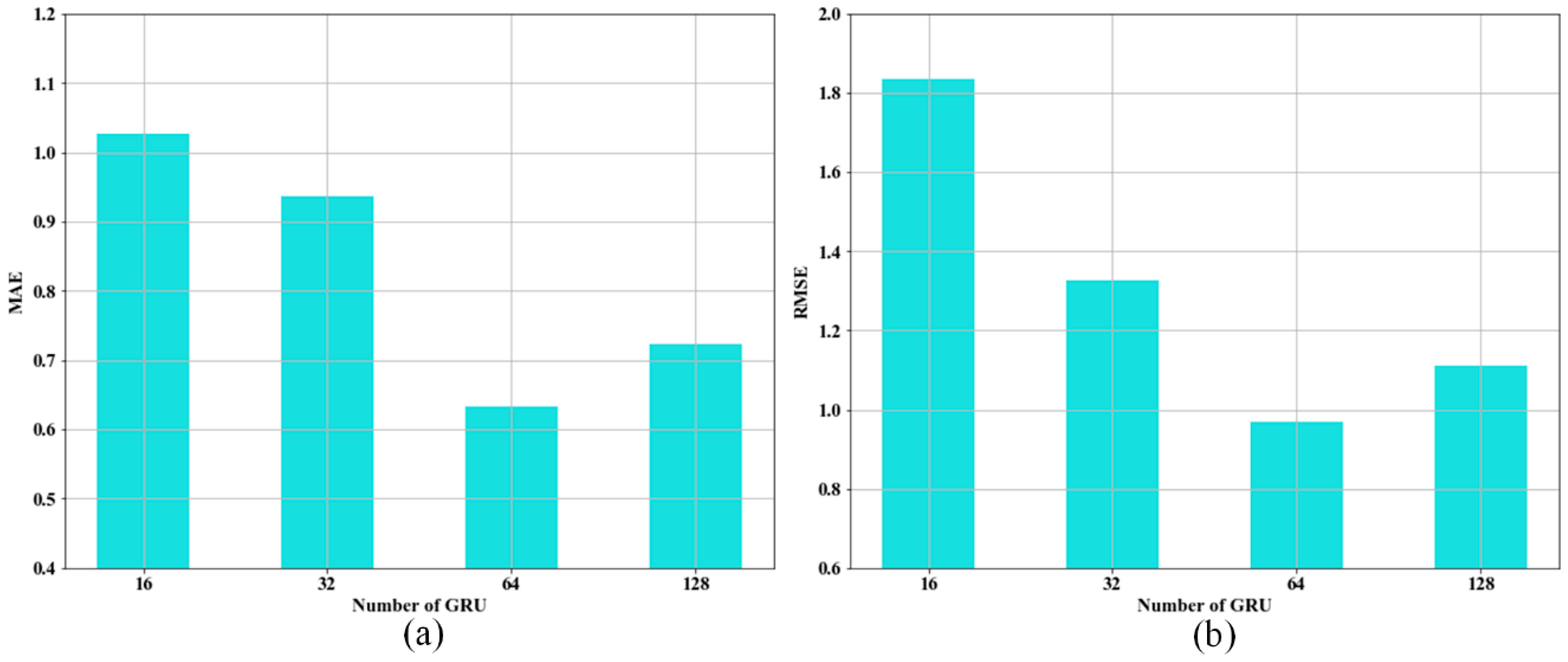
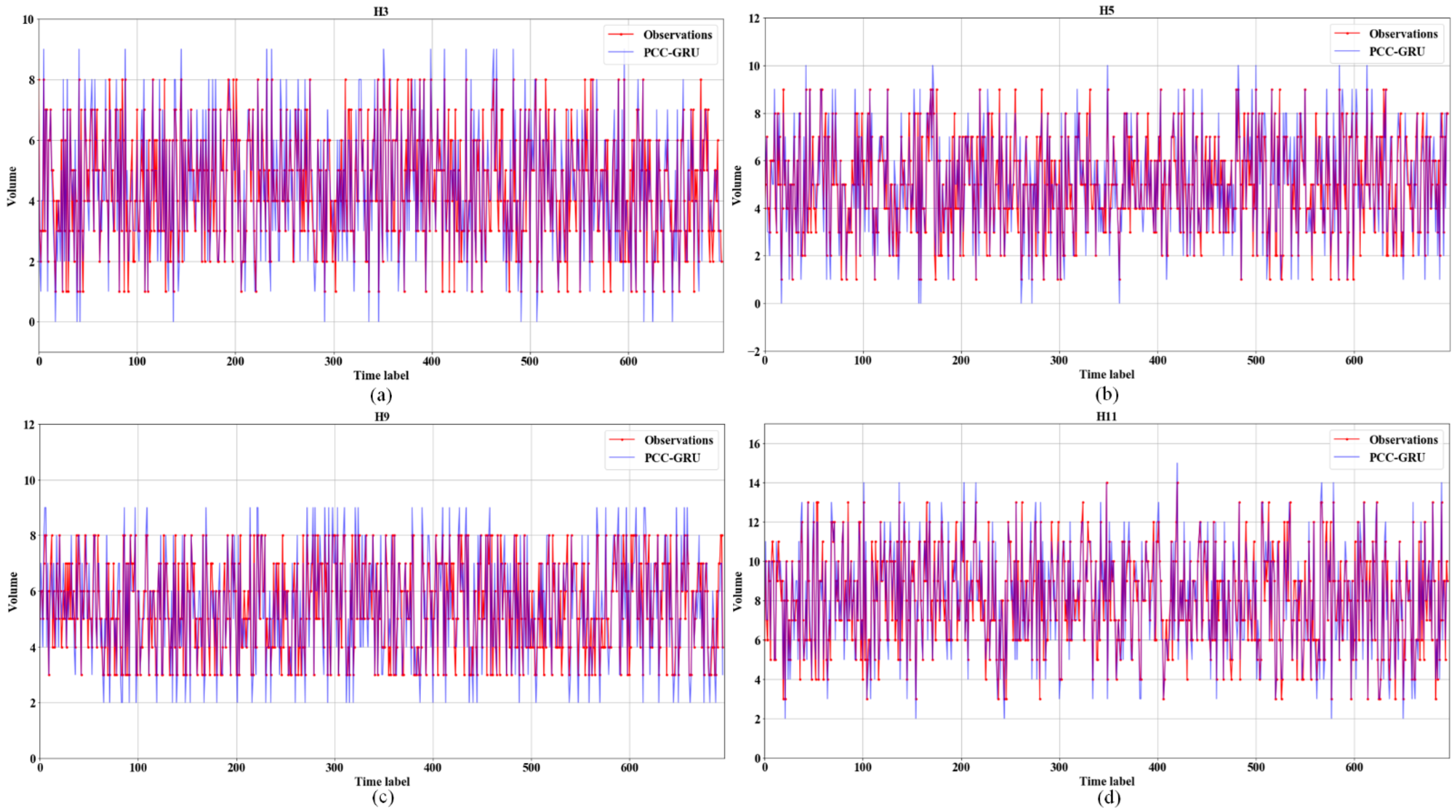
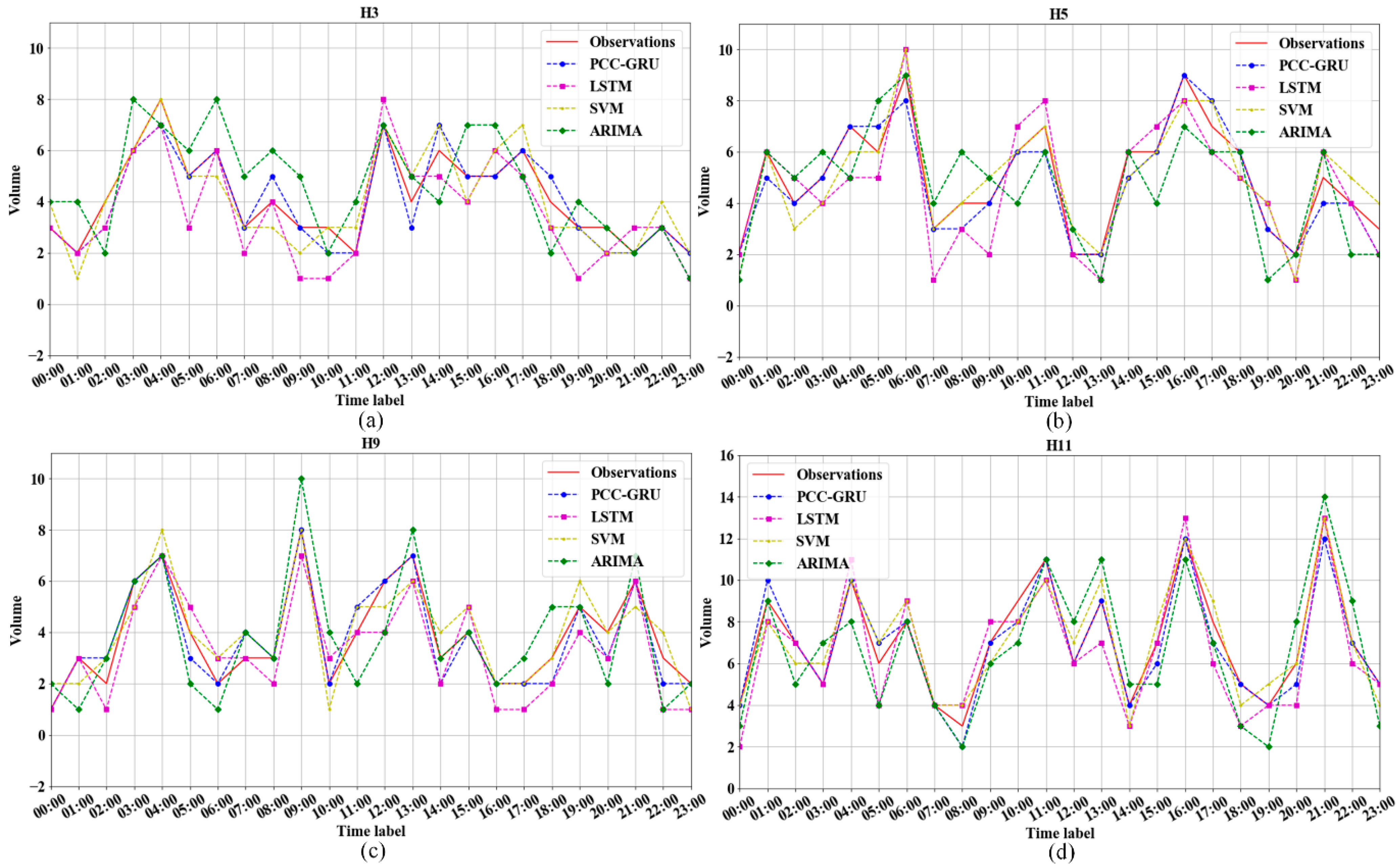
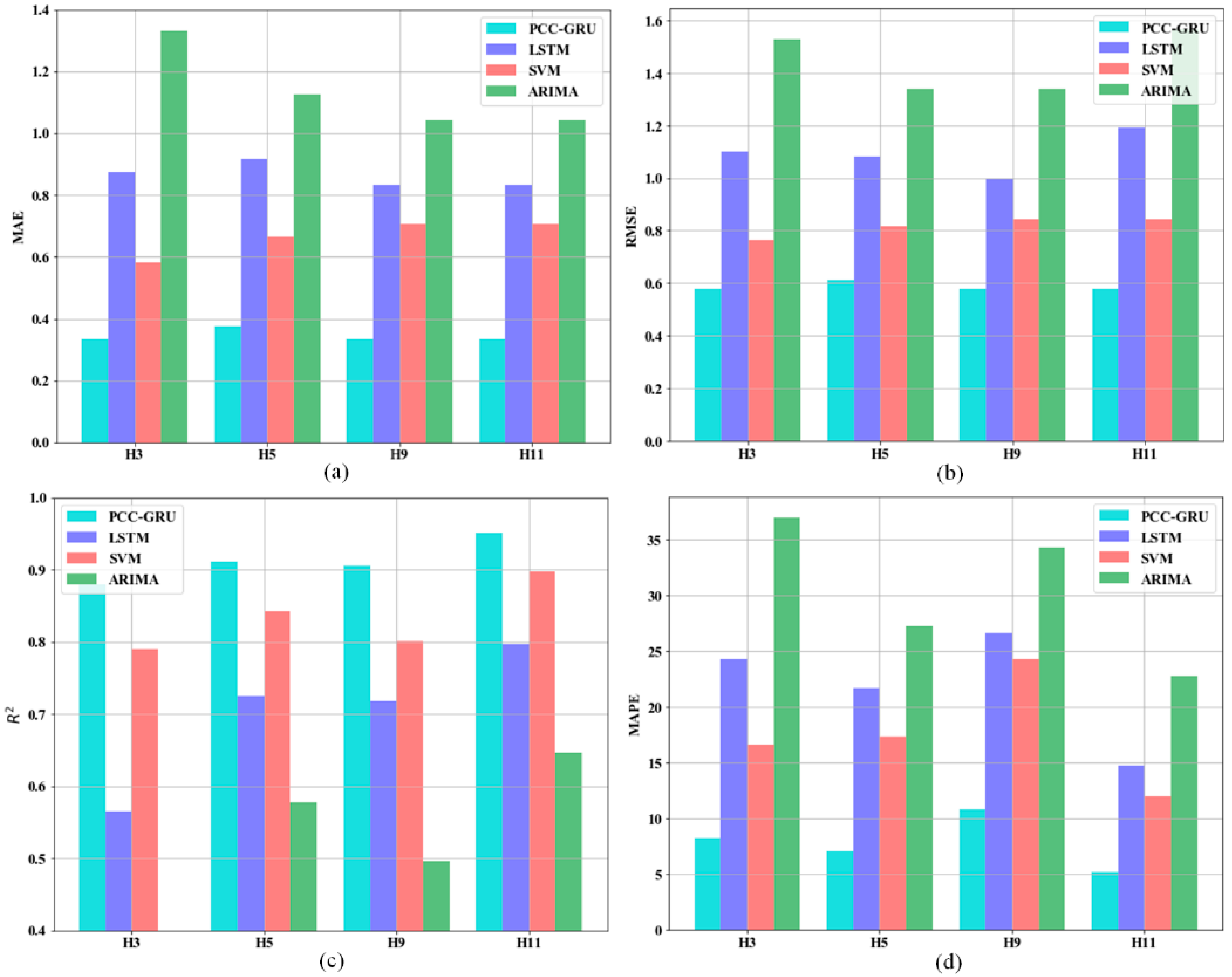
4.2. Results and Analysis

The data of four sections (H3, H5, H9, and H11) were selected to verify the method proposed in this research. In order to set the optimal threshold of PCC and time steps in the GRUs, many experiments were carried out in this research. Indicators for evaluating the experimental results can be calculated using Equations (10)–(13). In these equations, x_i is the temporary ship traffic volume value measured on 30 March 2021, while p_i is the predicted value by PCC–GRU, calculated with different parameters.

To study the influence of spatiotemporal state variables on prediction accuracy and determine the optimal parameters, the thresholds of PCC were set as 0.8, 0.7, 0.6, and 0.5, because when the threshold is greater than or equal to 0.8, there is no section related to H3, H5, H9, or H11 in space. To improve the prediction accuracy, the PCC algorithm was used to select spatial characteristic variables. From the position of each observation section, it can be seen that the sections with a large correlation and with the target section are located in the water area around the target, indicating that the traffic flow of the surrounding water area has a great impact on the target section. According to the actual situation, the effectiveness of the PCC algorithm in spatial feature variable selection was verified. Timesteps are an import parameter in neural networks. If the number of timesteps is n, that means that we think that each value is related to n values in front of it. If the timestep used in prediction is too large, it will lead to time information redundancy and affect the accuracy of the prediction results. If the timestep is too small, it will lead to overfitting of the model. The performance of the model can be seen in

Table 4. Prediction performance of different thresholds in H3.

Threshold	Section Related to H3	Time Steps	MAE	RMSE	MAPE	R2
0.8	/	3	1.61207	1.75961	42.58056	0.16006
		4	1.16523	1.38184	34.99692	0.48199
		5	0.69115	0.82319	18.32865	0.71491
		6	0.67851	0.80884	19.62209	0.81716
		7	0.65454	0.78254	18.45094	0.82826
0.7	H1 H5	3	1.47985	1.69798	41.62103	0.15091
		4	1.16954	1.38582	33.64929	0.47622
		5	0.70286	0.88204	20.64433	0.82194
		6	0.66256	0.83853	19.73351	0.80314
		7	0.65273	0.74592	18.75563	0.81522
0.6	H1 H5 H8	3	1.31057	1.68343	39.71651	0.13742
		4	1.20977	1.30272	36.35331	0.45431
		5	0.66667	0.81497	20.85102	0.81914
		6	0.66667	0.76497	19.59404	0.88914
		7	0.53453	0.68563	10.65256	0.90365
0.5	H1 H5 H8	3	1.31057	1.68343	39.71651	0.13742
		4	1.20977	1.30272	36.35331	0.45431
		5	0.66667	0.81497	20.85102	0.81914
		6	0.66667	0.76497	19.59404	0.88914
		7	0.53453	0.68563	10.65256	0.90365

,

Table 5. Prediction performance of different thresholds in H5.

Threshold	Section Related to H5	Time Steps	MAE	RMSE	MAPE	R2
0.8	/	3	1.58275	1.76979	38.51897	0.22023
		4	1.21120	1.41877	30.82569	0.49887
		5	0.67241	0.82000	16.96503	0.83260
		6	0.66235	0.81385	16.22976	0.83510
		7	0.64080	0.80765	16.31632	0.83760
0.7	H3 H8	3	1.41724	1.75878	38.06598	0.39443
		4	1.16666	1.39777	29.46423	0.51568
		5	0.66816	0.81505	16.21954	0.83117
		6	0.63662	0.79003	15.56588	0.84225
		7	0.63345	0.72873	15.60616	0.85674
0.6	H1 H3 H8	3	1.39669	1.69558	36.73457	0.32426
		4	1.16373	1.33858	28.51531	0.59998
		5	0.66104	0.80524	15.78878	0.82455
		6	0.64689	0.78769	13.30716	0.89652
		7	0.62234	0.71074	9.47337	0.91359
0.5	H1 H3 H8	3	1.39669	1.69558	36.73457	0.32426
		4	1.16373	1.33858	28.51531	0.59998
		5	0.66104	0.80524	15.78878	0.82455
		6	0.64689	0.78769	13.30716	0.89652
		7	0.62234	0.71074	9.47337	0.91359

,

Table 6. Prediction performance of different thresholds in H9.

Threshold	Section Related to H9	Time Steps	MAE	RMSE	MAPE	R2
0.8	/	3	1.48127	1.86125	30.61857	0.23653
		4	1.22701	1.42535	25.32567	0.30146
		5	0.68241	0.83008	14.76454	0.76802
		6	0.67965	0.82055	13.19848	0.77274
		7	0.66523	0.81516	12.53072	0.78172
0.7	H6	3	1.46275	1.85476	29.59729	0.25606
		4	1.12356	1.37632	23.55022	0.34897
		5	0.66839	0.82769	13.284	0.77004
		6	0.61092	0.82319	13.10851	0.78238
		7	0.60939	0.80334	12.46232	0.79934
0.6	H4 H6	3	1.45873	1.80834	31.70823	0.272437
		4	1.10492	1.37089	23.86203	0.367155
		5	0.63366	0.82304	14.44496	0.81392
		6	0.61264	0.82218	14.5587	0.83497
		7	0.60034	0.80091	11.53072	0.85034
0.5	H2 H4 H6	3	1.42701	1.76694	30.44643	0.27749
		4	1.10471	1.36167	24.53903	0.36465
		5	0.62425	0.78569	12.67354	0.84606
		6	0.58977	0.77932	11.04543	0.89926
		7	0.56942	0.75345	9.59432	0.92342

and

Table 7. Prediction performance of different thresholds in H11.

Threshold	Section Related to H11	Time Steps	MAE	RMSE	MAPE	R2
0.8	/	3	1.51585	1.78957	21.30284	0.39355
		4	1.21831	1.42137	16.93147	0.58054
		5	0.67381	0.82084	10.42556	0.69343
		6	0.64799	0.80493	9.12566	0.79752
		7	0.62345	0.79238	8.70294	0.80071
0.7	H8	3	1.50861	1.77856	21.14639	0.45469
		4	1.17674	1.39735	16.42899	0.61225
		5	0.68965	0.81455	10.25764	0.79094
		6	0.66667	0.80497	9.05628	0.74576
		7	0.61225	0.75934	8.57453	0.83634
0.6	H8 H9	3	1.48741	1.74551	20.91039	0.48333
		4	1.12575	1.33582	15.97794	0.67957
		5	0.65062	0.80676	10.17630	0.79775
		6	0.62077	0.79132	8.80699	0.83894
		7	0.60225	0.76385	8.53494	0.85846
0.5	H5 H8 H9	3	1.42989	1.76357	18.58104	0.56642
		4	1.06954	1.31858	13.15588	0.69508
		5	0.61793	0.76473	9.267573	0.85563
		6	0.58345	0.72785	8.238327	0.89162
		7	0.52425	0.68346	7.33485	0.92125

, where the timestep of 7 obtains the lowest error. Therefore, we set the timestep to 7 in our experiments.

Further analysis of the impact of timestep on prediction accuracy shows that the selection of different parameter combinations will change the prediction accuracy of the model. Within a certain range, the prediction accuracy is positively correlated with the timestep. In a certain range, with the decrease in the spatial threshold, the spatial correlation between observation sections is lower. In the case of a high threshold, too little information on other sections leads to a poor prediction effect. In the case of a low threshold, too much irrelevant information is added to interfere with the prediction effect. Based on the prediction performance of different thresholds in Table 4, Table 5, Table 6 and Table 7, the threshold was set to 0.5, 0.5, 0.6, and 0.6, respectively. The predicted and true values of observation sections H3, H5, H9, and H11 in the training dataset are shown in Figure 6; the predicted results are in good agreement with the actual values, indicating that the PCC–GRU model is feasible in the actual traffic scenario.

To verify the prediction performance of the PCC–GRU model, comparative experiments were set up in this study. LSTM, SVM, and ARIMA were used to predict the traffic flow of H3, H5, H9, and H11. These methods are commonly used in maritime traffic flow prediction [62,63,64]; therefore, these methods were used as benchmarking methods. After many experiments, the parameters of each model in the experiment were determined, as shown in

Table 8. Parameter setting of models.

Model	Parameter
LSTM	Neuron	12
	Timesteps	5
	Number of Iterations	300
SVM	Kernel Function	Radial Basis Function
	Penalty Factor	0.8
	Number of Iterations	500
ARIMA	Autoregressive Terms	2
	Moving average Terms	6
	Difference Items	1

. The prediction results of the ship traffic flow of each model are shown in Figure 7.

It can be seen from

Table 9. Performance comparison of different models.

	Models	Evaluation Indexes
		MAE	RMSE	MAPE	R2
H3	PCC–GRU	0.3333	0.5774	8.1597	0.8799
	ARIMA	0.8750	1.0992	24.2411	0.5647
	SVM	0.5833	0.7638	16.5972	0.7899
	LSTM	1.3333	1.5275	36.9792	0.1595
H5	PCC–GRU	0.3750	0.6124	7.0006	0.9116
	ARIMA	0.9167	1.0801	21.6402	0.7250
	SVM	0.6667	0.8165	17.3247	0.8429
	LSTM	1.1250	1.3385	27.1957	0.5774
H9	PCC–GRU	0.3333	0.5774	10.7639	0.9063
	ARIMA	0.8333	1.0000	26.6022	0.7188
	SVM	0.7083	0.8416	24.2640	0.8008
	LSTM	1.0417	1.3385	34.2758	0.4961
H11	PCC–GRU	0.3333	0.5774	5.1403	0.9521
	ARIMA	0.9167	1.1902	14.7058	0.7964
	SVM	0.7083	0.8416	11.9562	0.8982
	LSTM	1.3750	1.5679	22.7626	0.6466

that different models have different results in the traffic flow prediction experiment in the wind farms water area. In our case study, the LSTM model did not take into account the spatial information in the data, so its prediction accuracy was lower than that of the PCC–GRU model, and the time taken to train the LSTM model was too long for real-time prediction of maritime traffic flow. The machine learning algorithm SVM is suitable for short-term traffic forecasting, but the output of the SVM model will oscillate as the training data and the forecasting time increase. Meanwhile, the linear model ARIMA is unable to identify the randomness and nonlinearity in the data, making it difficult to make accurate predictions of random changes in traffic. The MAE of the PCC–GRU model in the prediction experiments of the four sections (H3, H5, H9, and H11) was 0.3333, 0.3750, 0.3333, and 0.3333, respectively; the RMSE of the PCC–GRU model of the four sections was 0.5774, 0.6124, 0.5774, and 5774, respectively, while the MAPE was 8.1597, 7.0006, 10.7639, and 5.1403, respectively, which is the smallest in the comparative analysis of the models. R² is usually used to describe the fitting degree of the data; the closer it is to 1, the better the fitting degree, and the smaller the deviation between the fitted curve and the original data points. The R² of the PCC–GRU model was 0.8799, 0.9116, 0.9063, and 0.9521, respectively, which was greater than that of other models. The bar chart of the error analysis indicators can be seen in Figure 8. In conclusion, the prediction results of the PCC–GRU model are closer to the observed values, and the performance of its algorithm is better than that of other traditional traffic flow prediction methods. The analysis of vessel traffic flow is the basis for evaluating the safety of vessel navigation in a given area of water. By predicting the ship traffic flow in the wind farms water area and maintaining real-time monitoring, it is possible to predict the business of vessel navigation and to control the traffic flow to avoid close-quarters situations.

5. Conclusions

According to the needs of traffic characteristic analysis and traffic supervision in complex waters, this study introduced the spatial correlation of ship traffic flow structure into machine learning based on the variant GRU of the recurrent neural network, constructing a spatiotemporal dependence characteristic matrix of ship traffic flow, and improving the prediction accuracy of the ship traffic flow by the neural network. The PCC algorithm is simple to implement and fast to compute, taking into account the degree of correlation of time series at different times, and it is suitable for determining correlation between random variables. The GRU uses a unique memory module instead of implicit nodes, which increases the robustness of the model and can effectively compensate for the shortcomings of traditional neural networks that cannot effectively process long time series. Taking the water area of the wind farm in the Yancheng sea area of Jiangsu Province as an example, the traffic flow in this area was predicted. Compared to results of the commonly used ship traffic flow prediction models ARIMA, SVM, and LSTM, the GRU method’s prediction was proven to be effective. The machine learning algorithm SVM is suitable for short-term prediction of traffic flows, but as the prediction time increases, the output of the SVM model will oscillate. The linear model ARIMA cannot identify the randomness and nonlinearity in the data, making it difficult to accurately predict the random changes in traffic. The LSTM model does not take into account the spatial information in the data, and therefore has a lower prediction accuracy than the PCC–GRU model.

By predicting the ship traffic flow and analyzing the temporal and spatial characteristics of traffic flow in complex waters, the marine traffic situation can be evaluated in real time, providing a theoretical basis for the risk evaluation and navigation safety guarantee of complex waters—especially the waters in wind farms with multi-route intersection—and reduces the risks of navigation and operation in the waters. Modelling the spatiotemporal dependence of ship traffic flow is a key area of future research. There are many factors affecting traffic flow prediction that have not been fully considered in this paper. The model proposed in this paper learns static spatial dependencies; however, the dependencies between locations may change over time. In subsequent research, dynamic structures should be considered in order to further improve the prediction performance.

References

1. Premalatha, M.; Abbasi, T.; Abbasi, S.A. Wind energy: Increasing deployment, rising environmental concerns. Renew. Sustain. Energy Rev. 2014, 31, 270–288. [Google Scholar]
2. Kusiak, A.; Song, Z. Design of wind farm layout for maximum wind energy capture. Renew. Energy 2010, 35, 685–694. [Google Scholar] [CrossRef]
3. Wang, X.Y.; Vilathgamuwa, D.M.; Choi, S.S. Determination of battery storage capacity in energy buffer for wind farm. IEEE Trans. Energy Convers. 2008, 23, 868–878. [Google Scholar] [CrossRef]
4. Jongbloed, R.H.; van der Wal, J.T.; Lindeboom, H.J. Identifying space for offshore wind energy in the North Sea. Consequences of scenario calculations for interactions with other marine uses. Energy Policy 2014, 68, 320–333. [Google Scholar] [CrossRef]
5. Frandsen, S.; Barthelmie, R.; Pryor, S.; Rathmann, O.; Larsen, S.; Højstrup, J.; Thøgersen, M. Analytical modelling of wind speed deficit in large offshore wind farms. Wind. Energy Int. J. Prog. Appl. Wind. Power Convers. Technol. 2006, 9, 39–53. [Google Scholar] [CrossRef]
6. Díaz, H.; Soares, C.G. Review of the current status, technology and future trends of offshore wind farms. Ocean Eng. 2020, 209, 107381. [Google Scholar] [CrossRef]
7. Hüppop, O.; Dierschke, J.; Exo, K.M.; Fredrich, E.; Hill, R. Bird migration studies and potential collision risk with offshore wind turbines. Ibis 2006, 148, 90–109. [Google Scholar] [CrossRef]
8. Dai, L.; Ehlers, S.; Rausand, M.; Utne, I.B. Risk of collision between service vessels and offshore wind turbines. Reliab. Eng. Syst. Saf. 2013, 109, 18–31. [Google Scholar] [CrossRef]
9. Ren, N.X.; Ou, J.P. A crashworthy device against ship-OWT collision and its protection effects on the tower of offshore wind farms. China Ocean Eng. 2009, 23, 594–602. [Google Scholar]
10. Furness, R.W.; Wade, H.M.; Masden, E.A. Assessing vulnerability of marine bird populations to offshore wind farms. J. Environ. Manag. 2013, 119, 56–66. [Google Scholar] [CrossRef]
11. Shafiee, M. A fuzzy analytic network process model to mitigate the risks associated with offshore wind farms. Expert Syst. Appl. 2015, 42, 2143–2152. [Google Scholar] [CrossRef]
12. Sun, H.; Liu, H.; Xiao, H.; He, R.; Ran, B. Use of local linear regression model for short-term traffic forecasting. Transp. Res. Rec. 2003, 1836, 143–150. [Google Scholar] [CrossRef]
13. Williams, B.M.; Hoel, L.A. Modeling and forecasting vehicular traffic flow as a seasonal ARIMA process: Theoretical basis and empirical results. J. Transp. Eng. 2003, 129, 664–672. [Google Scholar] [CrossRef] [Green Version]
14. Getahun, K.A. Time series modeling of road traffic accidents in Amhara Region. J. Big Data 2021, 8, 1–15. [Google Scholar] [CrossRef]
15. Guo, J.; Huang, W.; Williams, B.M. Adaptive Kalman filter approach for stochastic short-term traffic flow rate prediction and uncertainty quantification. Transp. Res. Part C Emerg. Technol. 2014, 43, 50–64. [Google Scholar] [CrossRef]
16. Xie, Y.; Zhang, Y.; Ye, Z. Short-term traffic volume forecasting using kalman filter with discrete wavelet decomposition. Comput.-Aided Civ. Infrastruct Eng. 2007, 22, 326–334. [Google Scholar] [CrossRef]
17. Saeedmanesh, M.; Kouvelas, A.; Geroliminis, N. An extended Kalman filter approach for real-time state estimation in multi-region MFD urban networks. Transp. Res. Part C Emerg. Technol. 2021, 132, 103384. [Google Scholar] [CrossRef]
18. Smith, B.L.; Demetsky, M.J. Forecasting freeway traffic flow for intelligent transportation systems application. Transp. Res. Part A Policy Pract. 1997, 31, 61. [Google Scholar]
19. Smith, B.L.; Williams, B.M.; Oswald, R.K. Comparison of parametric and nonparametric models for traffic flow forecasting. Transp. Res. Part C Emerg. Technol. 2002, 10, 303–321. [Google Scholar] [CrossRef]
20. Zheng, Z.; Su, D. Short-term traffic volume forecasting: A k-nearest neighbor approach enhanced by constrained linearly sewing principle component algorithm. Transp. Res. Part C Emerg. Technol. 2014, 43, 143–157. [Google Scholar] [CrossRef] [Green Version]
21. Wang, J.; Boukerche, A. Non-parametric models with optimized training strategy for vehicles traffic flow prediction. Comput. Netw. 2021, 187, 107791. [Google Scholar] [CrossRef]
22. Castillo, E.; Menéndez, J.M.; Sánchez-Cambronero, S. Predicting traffic flow using bayesian networks. Transp. Res. Part B Meth. 2008, 42, 482–509. [Google Scholar] [CrossRef]
23. Wang, J.; Deng, W.; Guo, Y. New Bayesian combination method for short-term traffic flow forecasting. Transp. Res. Part C Emerg. Technol. 2014, 43, 79–94. [Google Scholar] [CrossRef]
24. Afrin, T.; Yodo, N. A probabilistic estimation of traffic congestion using Bayesian network. Measurement 2021, 174, 109051. [Google Scholar] [CrossRef]
25. Qi, Y.; Ishak, S. A hidden Markov model for short term prediction of traffic conditions on freeways. Transp. Res. Part C Emerg. Technol. 2014, 43, 95–111. [Google Scholar] [CrossRef]
26. Rajawat, N.; Gupta, N.; Lalwani, S. A comprehensive review of hidden Markov model applications in prediction of human mobility patterns. Int. J. Swarm Intell. 2021, 6, 24–47. [Google Scholar] [CrossRef]
27. Zhang, C.; Chen, L. Traffic flow combining forecast model based on least squares support vector machine. J. Hunan Inst. Eng. 2010, 20, 56–58. [Google Scholar]
28. Wang, J.; Shi, Q. Short-term traffic speed forecasting hybrid model based on Chaos-Wavelet analysis-support vector machine theory. Transp. Res. Part C Emerg. Technol. 2013, 27, 219–232. [Google Scholar] [CrossRef]
29. Hu, Y.; Wu, C.; Liu, H. Prediction of passenger flow on the highway based on the least square support vector machine. Transp. Res. J. Vilnius Gedim. Tech. Univ. Lith. Acad Sci. 2011, 26, 197–203. [Google Scholar]
30. Castro-Neto, M.; Jeong, Y.S.; Jeong, M.K.; Han, L.D. Online-SVR for short-term traffic flow prediction under typical and atypical traffic conditions. Expert Syst. Appl. 2009, 36, 6164–6173. [Google Scholar] [CrossRef]
31. Asif, M.T.; Dauwels, J.; Chong, Y.G.; Oran, A.; Fathi, E.; Xu, M. Spatiotemporal patterns in large-scale traffic speed prediction. IEEE Trans. Intell. Transp. Syst. 2014, 15, 794–804. [Google Scholar] [CrossRef] [Green Version]
32. Yao, B.; Yao, J.; Zhang, M.; Yu, L. Improved support vector machine regression in multi-step-ahead prediction for rock displacement surrounding a tunnel. Sci. Iran. 2014, 21, 1309–1316. [Google Scholar]
33. Toan, T.D.; Truong, V.H. Support vector machine for short-term traffic flow prediction and improvement of its model training using nearest neighbor approach. Transp. Res. Rec. 2021, 2675, 362–373. [Google Scholar] [CrossRef]
34. Hong, H.; Huang, W.; Xing, X.; Zhou, X. Hybrid multi-metric K-nearest neighbor regression for traffic flow prediction. In Proceedings of the 2015 IEEE 18th International Conference on Intelligent Transportation Systems, Gran Canaria, Spain, 15–18 September 2015; pp. 2262–2267. [Google Scholar]
35. Akbari, M.; Overloop, P.J.V.; Afshar, A. Clustered K nearest neighbor algorithm for daily inflow forecasting. Water Resour. Manag. 2011, 25, 1341–1357. [Google Scholar] [CrossRef] [Green Version]
36. Yu, B.; Song, X.; Guan, F.; Yang, Z.; Yao, B. K-nearest neighbor model for multiple-time-step prediction of short-term traffic condition. J. Transp. Eng. 2016, 142, 04016018. [Google Scholar] [CrossRef]
37. Du, W.; Zhang, Q.; Chen, Y.; Ye, Z. San urban short-term traffic flow prediction model based on wavelet neural network with improved whale optimization algorithm. Sustain. Cities Soc. 2021, 69, 102858. [Google Scholar] [CrossRef]
38. Li, L.; Yang, Y.; Yuan, Z.; Chen, Z. A spatial-temporal approach for traffic status analysis and prediction based on bi-lstm structure. Mod. Phys. Lett. B 2021, 35, 2150481. [Google Scholar] [CrossRef]
39. Wang, K.; Ma, C.; Qiao, Y.; Lu, X.; Hao, W.; Dong, S. A hybrid deep learning model with 1DCNN-LSTM-Attention networks for short-term traffic flow prediction. Phys. A 2021, 583, 126293. [Google Scholar] [CrossRef]
40. Chen, X.; Chen, H.; Yang, Y.; Wu, H.; Zhang, W.; Zhao, J.; Xiong, Y. Traffic flow prediction by an ensemble framework with data denoising and deep learning model. Phys. A 2021, 565, 125574. [Google Scholar] [CrossRef]
41. Cheng, Z.; Lu, J.; Zhou, H.; Zhang, Y.; Zhang, L. Short-Term Traffic Flow Prediction: An Integrated Method of Econometrics and Hybrid Deep Learning. IEEE Trans. Intell. Transp. Syst. 2021, 1–14. [Google Scholar] [CrossRef]
42. Zheng, H.; Lin, F.; Feng, X.; Chen, Y. A hybrid deep learning model with attention-based conv-LSTM networks for short-term traffic flow prediction. IEEE Trans. Intell. Transp. Syst. 2020, 22, 6910–6920. [Google Scholar] [CrossRef]
43. Li, H. Research on prediction of traffic flow based on dynamic fuzzy neural networks. Neural Comput. Appl. 2016, 27, 1969–1980. [Google Scholar] [CrossRef]
44. Huang, W.; Song, G.; Hong, H.; Xie, K. Deep architecture for traffic flow prediction: Deep belief networks with multitask learning. IEEE Trans. Intell. Transp. Syst. 2014, 15, 2191–2201. [Google Scholar] [CrossRef]
45. Yang, H.F.; Dillon, T.S.; Chen, Y.P. Optimized structure of the traffic flow forecasting model with a deep learning approach. IEEE Trans. Neural Netw. Learn. Syst. 2016, 28, 2371–2381. [Google Scholar] [CrossRef]
46. Lu, S.; Zhang, Q.; Chen, G.; Seng, D. A combined method for short-term traffic flow prediction based on recurrent neural network. Alex Eng. J. 2021, 60, 87–94. [Google Scholar] [CrossRef]
47. Ho, L.W.; Lie, T.T.; Leong, P.T.; Clear, T. Developing offshore wind farm siting criteria by using an international Delphi method. Energy Policy 2018, 113, 53–67. [Google Scholar] [CrossRef]
48. Noorollahi, Y.; Yousefi, H.; Mohammadi, M. Multi-criteria decision support system for wind farm site selection using GIS. Sustain. Energy Technol. Assess. 2016, 13, 8–50. [Google Scholar] [CrossRef]
49. Florian, M.; Sørensen, J.D. Risk-based planning of operation and maintenance for offshore wind farms. Energy Procedia 2017, 137, 261–272. [Google Scholar] [CrossRef]
50. Martin, R.; Lazakis, I.; Barbouchi, S.; Johanning, L. Sensitivity analysis of offshore wind farm operation and maintenance cost and availability. Renew. Energy 2016, 85, 1226–1236. [Google Scholar] [CrossRef] [Green Version]
51. Santos, F.P.; Teixeira, A.P.; Guedes Soares, C. Maintenance planning of an offshore wind turbine using stochastic Petri nets with predicates. J. Offshore Mech. Arct. Eng. 2018, 140, 021904. [Google Scholar] [CrossRef]
52. Höfer, T.; Sunak, Y.; Siddique, H.; Madlener, R. Wind farm siting using a spatial Analytic Hierarchy Process approach: A case study of the Städteregion Aachen. Appl. Energy 2016, 163, 222–243. [Google Scholar] [CrossRef]
53. Hooper, T.; Hattam, C.; Austen, M. Recreational use of offshore wind farms: Experiences and opinions of sea anglers in the UK. Mar. Policy 2017, 78, 55–60. [Google Scholar] [CrossRef] [Green Version]
54. Cervera, M.A.; Ginesi, A.; Eckstein, K. Satellite-based vessel Automatic Identification System: A feasibility and performance analysis. Int. J. Satell. Commun. Netw. 2011, 29, 117–142. [Google Scholar] [CrossRef]
55. Sang, L.Z.; Wall, A.; Mao, Z.; Yan, X.P.; Wang, J. A novel method for restoring the trajectory of the inland waterway ship by using AIS data. Ocean Eng. 2015, 110, 183–194. [Google Scholar] [CrossRef] [Green Version]
56. Benesty, J.; Chen, J.; Huang, Y.; Cohen, I. Pearson correlation coefficient. In Noise Reduction in Speech Processing; Springer: Berlin/Heidelberg, Germany, 2009; pp. 1–4. [Google Scholar]
57. Zuo, F.; Li, Y.; Johnson, S.; Johnson, J.; Varughese, S.; Copes, R.; Chen, H. Temporal and spatial variability of traffic-related noise in the City of Toronto, Canada. Sci. Total Environ. 2014, 472, 1100–1107. [Google Scholar] [CrossRef] [PubMed]
58. Fu, R.; Zhang, Z.; Li, L. Using LSTM and GRU neural network methods for traffic flow prediction. In Proceedings of the 2016 31st Youth Academic Annual Conference of Chinese Association of Automation (YAC), Wuhan, China, 11–13 November 2016; IEEE: Piscataway, NJ, USA; pp. 324–328. [Google Scholar]
59. Zhang, D.; Kabuka, M.R. Combining weather condition data to predict traffic flow: A GRU-based deep learning approach. IET Intell. Transp. Syst. 2018, 12, 578–585. [Google Scholar] [CrossRef]
60. Wang, S.; Zhao, J.; Shao, C.; Dong, C.D.; Yin, C. Truck traffic flow prediction based on LSTM and GRU methods with sampled GPS data. IEEE Access 2020, 8, 208158–208169. [Google Scholar] [CrossRef]
61. Cho, K.; Van Merriënboer, B.; Bahdanau, D.; Bengio, Y. On the properties of neural machine translation: Encoder-decoder approaches. arXiv 2014, arXiv:1409.1259. [Google Scholar]
62. Liang, M.; Zhan, Y.; Liu, R.W. MVFFNet: Multi-view feature fusion network for imbalanced ship classification. Pattern Recognit. Lett. 2021, 151, 26–32. [Google Scholar] [CrossRef]
63. Wang, Y.; Liao, W.; Chang, Y. Gated recurrent unit network-based short-term photovoltaic forecasting. Energies 2018, 11, 2163. [Google Scholar] [CrossRef] [Green Version]
64. Zheng, G.; Chai, W.K.; Katos, V.; Walton, M. A joint temporal-spatial ensemble model for short-term traffic prediction. Neurocomputing 2021, 457, 26–39. [Google Scholar] [CrossRef]
Figure 1. Logical framework in this study.
Jmse 10 00295 g001
Figure 2. Diagram of the model structure used in this research: (a) Whole structure of the model. (b) Basic structure of the GRU.
Jmse 10 00295 g002
Figure 3. Schematic diagram of the observation section in the Yancheng wind farm area.
Jmse 10 00295 g003
Figure 4. MAE and RMSE with the same number of GRUs: (a) MAE of the experiment. (b) RMSE of the experiment.
Jmse 10 00295 g004
Figure 5. The loss of different batch sizes.
Jmse 10 00295 g005
Figure 6. Prediction results of the PCC–GRU model: (a) Training data in H3. (b) Training data in H5. (c) Training data in H9. (d) Training data in H11.
Jmse 10 00295 g006
Figure 7. Comparison of prediction results of different models: (a) Prediction results in H3. (b) Prediction results in H5. (c) Prediction results in H9. (d) Prediction results in H11.
Jmse 10 00295 g007
Figure 8. Bar chart of the error analysis indicators: (a) MAE of five prediction results. (b) RMSE of five prediction results. (c) R2 of five prediction results. (d) MASE of five prediction results.
Jmse 10 00295 g008