1. Introduction
Generally, vessels berth with the assistance of thrusters or tugs. However, most ships sailing at sea are only equipped with main propellers and rudder devices, while some ships are equipped with either two independent aft thrusters or one main aft thruster and a rudder without any bow or side thrusters. The insufficient force on the sway direction makes it difficult to control the vessel, especially when berthing at a low speed. Therefore, solving this problem will help save investment and construction costs, reduce the weight of the system, and increase its flexibility and operating reliability during the design process of the ship [
1,
2]. Researchers usually regard the underactuated vessel mentioned above as a multi-input multi-output underactuated system [
3].
Solving the problem of underactuated vessel auto-berthing means stabilizing the ship at the pier by controlling its rudder and propeller. During this process, precisely controlling the vessel’s position and speed is the key to realizing safe berthing, especially the speed control. Due to the massive inertia of the ship, excessive speed margin will cause huge damage to the wharf and hull. Therefore, limiting the yaw rate within a certain range during berthing will be meaningful. Meanwhile, the underactuated vessel system will be affected by dynamic uncertainty due to low-speed ships, diving effects, and quay wall effects. Accurately estimating the dynamic uncertainty of the vessel motion system will bring the model closer to reality and make the test results more referential.
Intelligent algorithms, classic control, and a combination of the two are the most common way to tackle the problem of underactuated vessels auto-berthing. In terms of the intelligent algorithms, Artificial Neural Network (ANN) and Proximal Policy Optimization (PPO) [
4] are already used in auto-berthing research. As for the former, the training data are usually obtained manually by controlling the ship to a specific pier in advance and training the weights and biases of the ANN, which could help realize auto-berthing control in a specific wharf [
5]. However, this method cannot achieve vessel auto-berthing control in different ports without training data. To solve this problem, the works in [
6,
7] use coordinate conversion controller switching technology and a distance measurement system and controller with ship sub-routes to tackle the problems of geographic coordinate limitation, measurement accuracy, and repeated network training and improve the adaptability of ANN berthing controllers.
In terms of the classical control methods, the auto-berthing problem tends to be classified as a stabilization control problem, i.e., to design a control scheme that makes the vessel stable in a certain position and state. Direct Liapunov method [
8,
9] and sliding mode control [
10] are the most common methods applied to realize auto berthing. In [
8], an auto-berthing controller based on concise backstepping was proposed. Bu [
10] designed a dynamic feedback controller and applied the recursive decomposition iterative method to tackle the underactuated vessel control problem. However, classical control theories are all based on the precise model of the controlled object. Thus, when the vessel berths at a low speed, the underactuated vessel system is affected by dynamic uncertainty.
In summary, whether intelligent algorithms are applied to implement ship berthing controllers or simple classical control methods are limited by the need for accurate mathematical models of ships, offline data training, or data consistency issues will occur, thus causing certain limitations to the engineering application of the controller. Therefore, researchers have been trying to combine the advantages of the two methods, which mainly focus on the control itself and berthing path planning. From the perspective of ship berthing control, in [
11], proportional derivative (PD) control was introduced into the ANN berthing controller designation to tackle the problem of training data consistency during auto berthing. In [
12], controllers are proposed that realized ship auto-berthing in a turn-around way and solved the dynamic uncertainty with RBF. From the perspective of berthing path planning, a controller based on Immune Memory-Particle Swarm Optimization (IM-PSO) is proposed to optimize the proportional integral derivative control parameters of berthing path tracking [
13]. An extended dynamic window approach for the automatic berthing of underactuated surface vessels [
14] could realize the automatic berthing under the influence of wind loads and obstacles. Han [
15] introduced a layered artificial potential field method to the berthing trajectory planning to tackle the problem of excessive turning of the berthing trajectory. The research mentioned above mainly focuses on the steady-state characteristics of the underactuated vessel motion control system but pays less attention to the transient performance, which might cause a collision with nearby vessels as discussed in [
16]. Dai et al. [
17] pointed out that when a ship is operating in a narrow waterway, the force will change. The system state will be restricted, i.e., the output or state of the ship is not allowed to exceed a certain constraint distance of the reference trajectory path, which is similar to a finite time control method [
18] proposed based on barrier Lyapunov function realized course keeping to improve control performance significantly. Tee, K.P., et al. [
19] used barrier Lyapunov to tackle the problem of restricted location during berthing. With the full-drive system with state constraints or output constraints as the research object [
20], the barrier Lyapunov function is used to reach infinity when its parameters are close to the constraint boundary, and stable control of the constraint system is realized. However, the above research does not involve the attempt to limit the speed in automatic berthing, which is very important for safe berthing.
Given the above, this paper focuses on solving the auto-berthing of underactuated surface vessels in the presence of uncertain dynamics and yaw rate limitation. The differential homeomorphism transformation approach is applied to convert the vessel to a cascade form. The RBF network estimates the unknown nonlinear functions. Furthermore, a filter based on dynamic surface control (DSC) is constructed. An auto-berthing control scheme is derived by combining minimum learning parameters technique (MLP), RBF, DSC, and applying the BLF method. The Lyapunov theory proves the stability. The significance of this paper can be summarized as follows.
- (1)
A novel auto-berthing control scheme considering BLF is proposed to successfully restrict the yaw rate within a smaller range during ship berthing, which has essential safety significance for real ship berthing.
- (2)
The vessel model dynamic uncertainty caused by underactuation has been fully solved using the RBF. This is compared with the research in [
8] that, without considering vessel model dynamic uncertainty, showed that an adaptive control scheme based on RBF can effectively approximate the unknown term and keep the output bounded.
The rest of this paper is organized as follows. The
Section 2 is the preliminary introduction. The
Section 3 introduces the process of the underactuated problem of the ship motion model with uncertain dynamics. The
Section 4 presents the design of the automatic berthing controller using the BLF, RBF, DSC, and MLP. The
Section 5 shows the simulation results and discussion. The last part presents conclusions and prospects for further research.
3. Problem Formulation
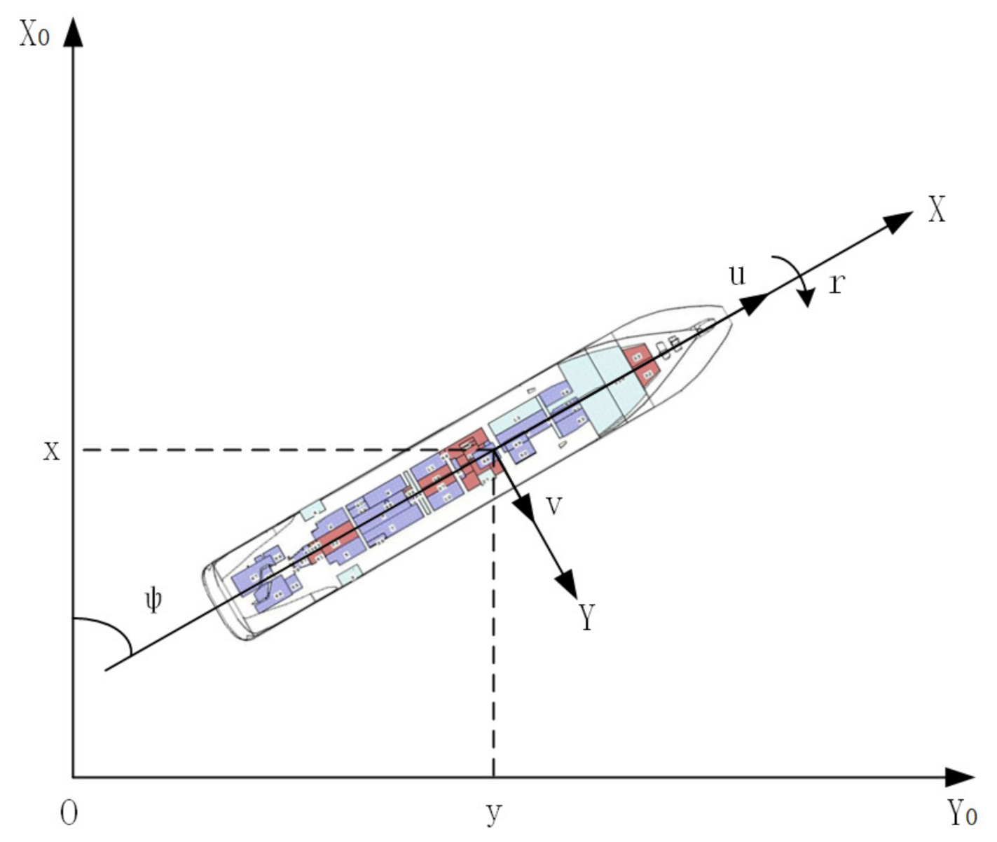
In general, the three degrees of freedom (3-DOF) underactuated marine surface vessel motion model can be described as in [
24], as shown in
Figure 1.
where
-denotes the vehicles’ position and heading.
denotes the surge, sway, and yaw velocities in the body-fixed frame.
denotes the actual input vector.
,
are hydrodynamic damping.
are unknown time-varying disturbance.
To solve the underactuated problem of the marine surface vessel model, the following differential homeomorphism transformation is introduced [
25]:
where
.
Taking the time derivative of Equation (
8), one can get
satisfies the following properties:
where
.
Furthermore, the mathematical model of underactuated marine surface vessel after differential homeomorphism transformation can be obtained as
where
,
,
are unmodeled dynamics.
Let
, then Equation (
11) can be written as
Further, convert system Equation (
12) into a chain structure system by introducing the following variable substitution and feedback transformation [
26]:
Next,
, let
, we have
Let
, the system Equation (
14) can be described as
As Equation (
15) is converted from Equation (
11), so if the stability of the system Equation (
15) and system Equation (
11) are same. In other words, when
, if
,
, will gradually stable at the origin.
Theorem 1 ([
27])
. For Equation (15), when , if , converges to zero, we have Then, Equation (14) can be simplified asLet , , , , we have According to Theorem 1, if system Equation (
17) gradually stabilizes, the system Equation (
15) will gradually stabilizes as well. Therefore, the remain work is make system Equation (
17) stable.
5. Simulation
In the simulation studies, model vessel named “Cyber ship I” is used to verify the effectiveness of the proposed control scheme. The parameters of “Cyber ship I” can be found in [
29]:
, ship length
m,
,
,
,
,
,
. In the simulation, The design parameters are
,
,
,
,
,
,
,
,
= 0.01,
= 0.01,
,
The initial states of the vessel is designed as
,
,
,
,
.
In addition, to verify the effectiveness of the control scheme designed in this paper, a comparison is made between the adaptive control considering BLF and the adaptive control without BLF. The adaptive control scheme without BLF is listed in Equation (
62). The initial states of the vessel model system setting are taken to be the same as the control scheme designed in this paper, and the parameters are
,
. The result of the simulation is shown in
Figure 2 and
Figure 3.
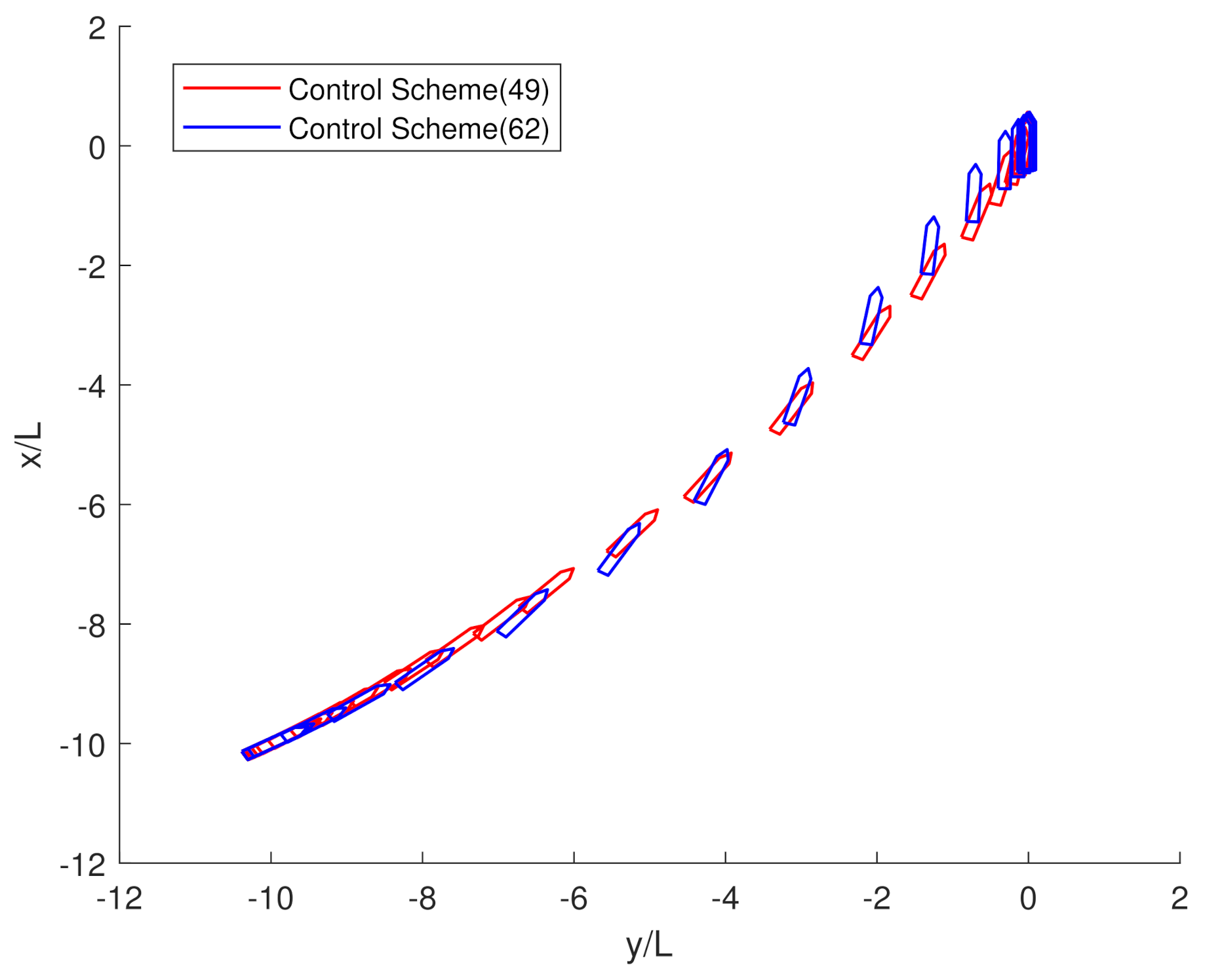
Figure 2 shows the trajectory comparison of the vessel with control scheme Equation (
49) and control scheme Equation (
62). It can be seen from this graph that both schemes helped the vessel realize berthing successfully.
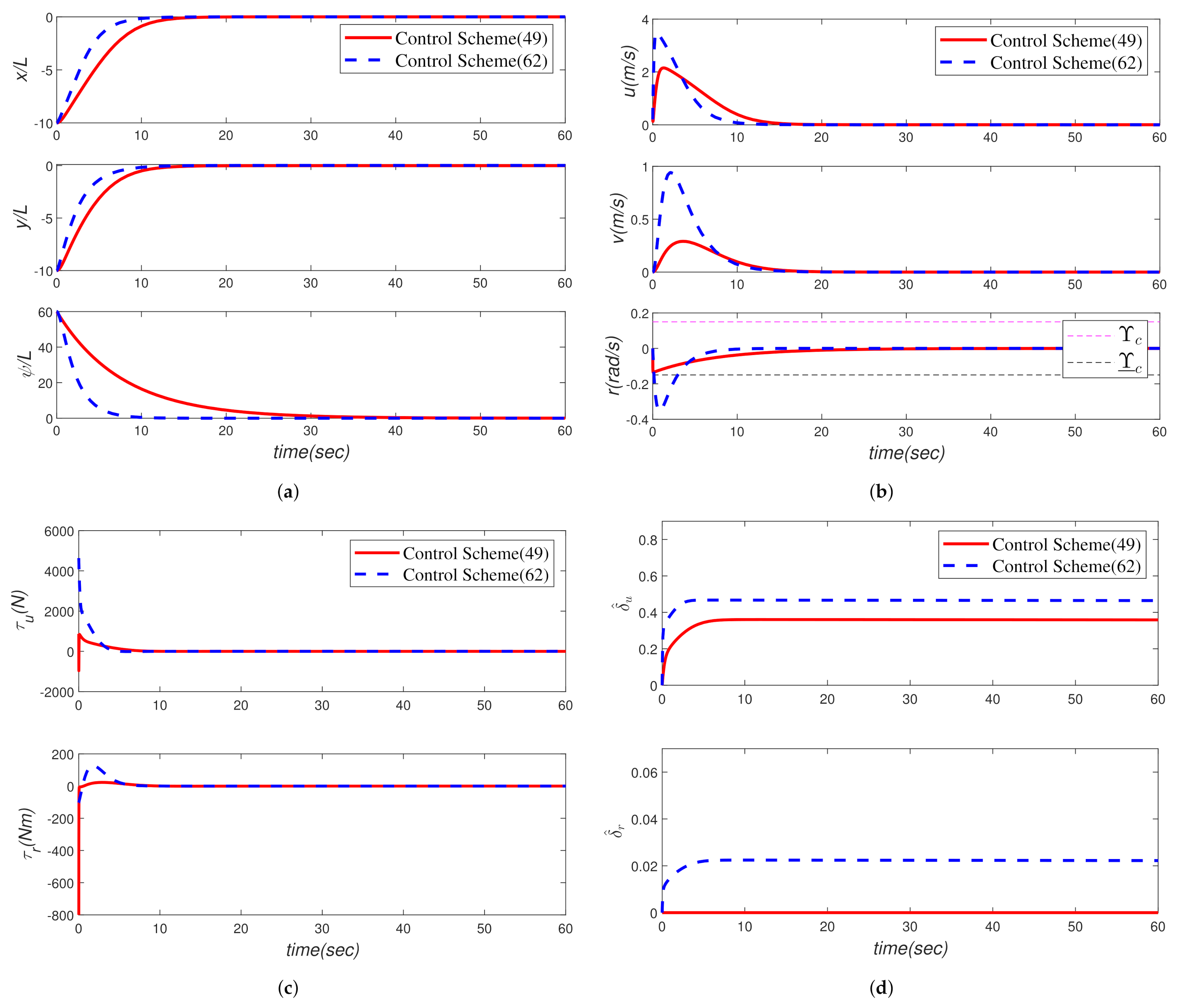
Figure 3a shows curves of vessel position and heading angle. The vessel under the control scheme (
49) reaches the desired lateral position
x = 0 at 17.27 s, and the longitudinal position reaches the desired position
y = 0 at 19.49 s, while the vessel under the control scheme Equation (
62) reaches desired position of lateral and longitudinal at 14.28 s and 16.09 s, respectively. In terms of heading, the vessel under control scheme Equation (
62) sharply decreases to 3.9° in 5.7 s, then gradually decreases and stabilizes at 0°. In contrast, the value of the vessel heading under control scheme Equation (
49) has been used for 43.59 s from 60° to 0°. It can be seen that the curve changes more smoothly.
Figure 3b displays curves change of surge velocity (
u), sway velocity (
v), and yaw rate (
r). For the vessel with a control scheme (
62), the acceleration phase of
u is from 0 to 0.6 s, and the maximum speed is 3.48 m/s, then it is reduced to 0 m/s in about 15 s, while the vessel under control scheme Equation (
49) reaches the maximum velocity of 2.15 m/s at approximately 2.15 s. Compared to
u,
v does not need to be too big in the process of vessel berthing for the vessel with control scheme Equation (
62), sway speed
v reaches the peak value of 0.94 m/s at around 2.4 s, decreases to 0 m/s, and stays stable at 18.87 s, while the sway speed
v of the vessel is under control scheme Equation (
49) reaches the maximum velocity of 0.29 m/s and stays stable at around 3.19 s. Through the comparison of the yaw rate (
r), it can be seen that the vessel controlled by the control scheme (
49) reaches a stable position in 26 s, and the value of
r is within (−0.15 rad/s − 0.15 rad/s) during the whole process, while the yaw rate of vessel controlled by the control scheme Equation (
62) exceeds 0.15 rad/s at around 0.16 s and reaches its peak value of 0.35 rad/s at around 0.6 s. Obviously, from the comparison result of the yaw rate, it can be seen that the control scheme with BLF can better limit the yaw rate within a certain range which verifies the effectiveness of our proposed control scheme.
Figure 3c illustrates the curves change of force and control force moment. It can be seen from the simulation image that the surge control force with control scheme Equation (
49) changes sharply increase from −959.8 N to 869.2 N and then gradually stabilize at 0 N in 10.9 s. The yaw control force moment changes from −1089 Nm to 22.97 Nm within approximately 2.4 s and gradually decreases to 0 Nm at 11.83 s. In contrast, the simulation image that the surge control force with control scheme Equation (
62) changes from 4653 N to −10 N in 6.5 s and gradually stabilizes at 0 N. The yaw control force moment reaches a peak value of 127 Nm at around 1.78 s and gradually decreases to 0 Nm at 9.7 s. The change of control force and torque is reasonable and bounded, which shows the effectiveness of the control rate designed in this paper.
Figure 3d shows the change of the adaptive parameters. It can be seen from the figure that the adaptive parameters are bounded and stable.
In short, it can be seen from
Figure 2 and
Figure 3 that the control scheme designed in this paper can effectively limit the yaw rate in a particular range, which meets the project’s needs.
In order to further verify the robustness of the control scheme, under the condition that the initial state of the ship and the design parameters of the control scheme remain unchanged, the bounded disturbance is selected for simulation test, and the disturbance vector is selected as
.
Figure 4 and
Figure 5 present the simulation results, which are used to analyze the control performance and system robustness.
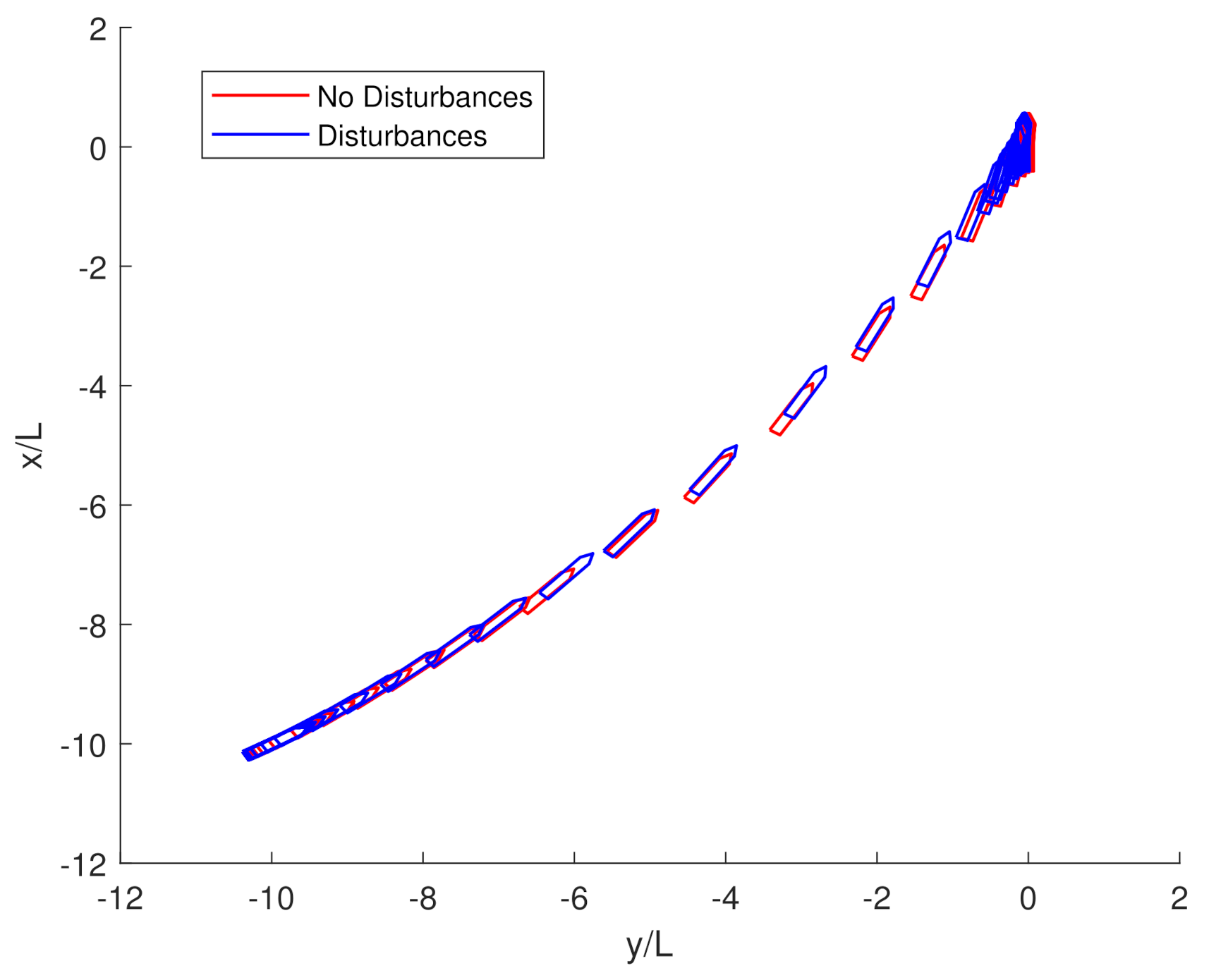
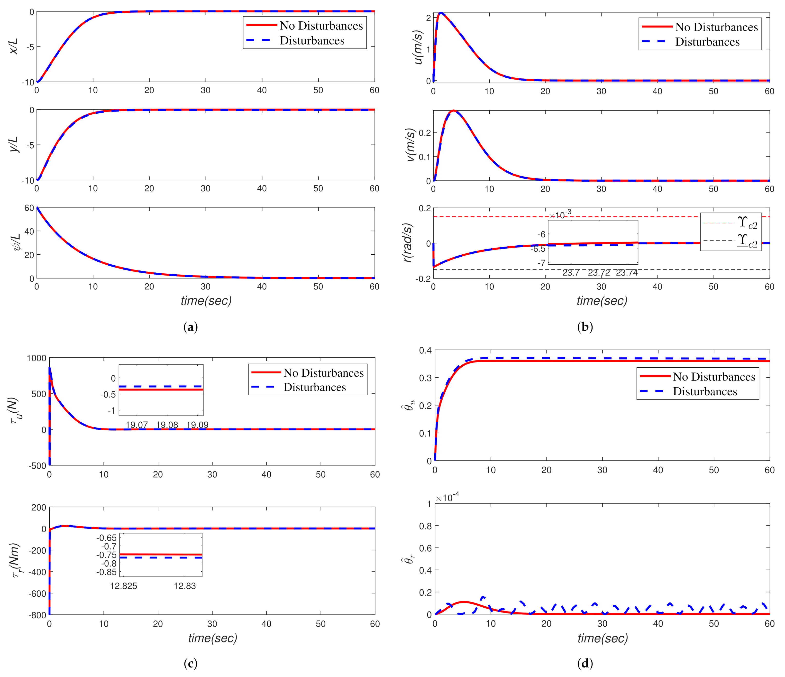
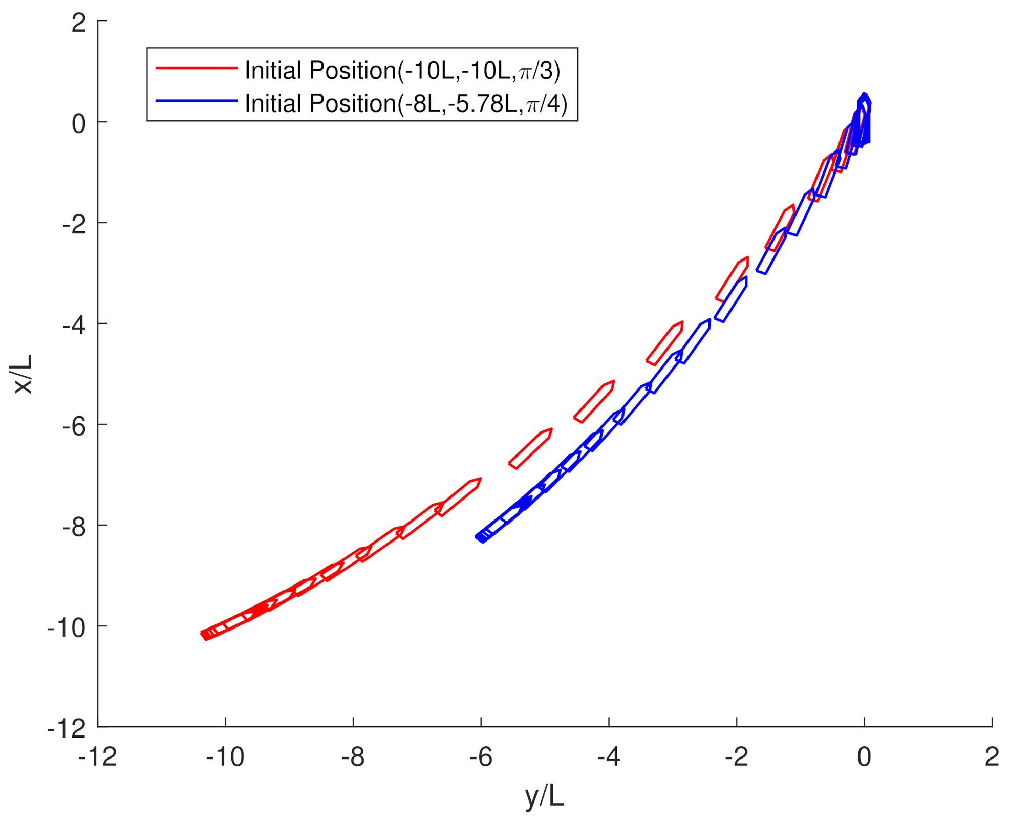
Figure 4 compares the results of trajectory with control scheme Equation (
49) under disturbance (indicated by a blue line) and without disturbance (indicated by a red line). It can be found that both berthing tasks are well finished.
Figure 5a shows curves of vessel position and heading angle. There is no overshoot in the two curves in the figure. Compared to the red line, the vessel’s position showed a slight deviation, and the curve of heading angle appeared fluctuations within a small bounded range between 0.13 rad/s to 0.02 rad/s after approximately 40 s.
Figure 5b demonstrates the comparison of the curves of surge velocity (
u), sway velocity (
v), and yaw rate (
r) of the vessel controlled by control scheme Equation (
49) and control scheme Equation (
49) with disturbance. For control scheme Equation (
49) with disturbance, the acceleration phase of
u is from 0 to 1.4 s, the maximum speed is 2.14 m/s at 1.41 s, then reduced to a stable scale between −0.00013 m/s to 0.00013 m/s in 26 s, while the sway velocity (
v) stabilized in a small bounded range between from −0.00025 m/s to 0.00025 m/s after approximately 26 s. By comparing the yaw rate (
r), the value of the yaw rate is within [−0.15 rad/s −0.15 rad/s] during the whole process, even under the influence of disturbance. It can be seen that in the case of interference, the berthing speed curve can still be stabilized within a small range. It is very close to the curve without interference, indicating that the system has certain robustness.
Figure 5c illustrates the curves change of force and control force moment of the vessel controlled by control scheme Equation (
49) without disturbance and control scheme Equation (
49) with disturbance. It can be seen from the image that the surge control force, which is indicated by a blue line, sharply increases from −2789 N to 876.7 N and then gradually stabilizes in a small bounded range between −0.01 N to 0.01 N after approximately 12 s. The yaw control force moment changes from −1089 Nm to 22.73 Nm within around 2.94 s and gradually decreases the small bounded range between −0.014 Nm to 0.014 Nm.
Figure 5d shows the change of the adaptive parameters. It can be seen that the (with disturbance indicated by a blue line) reaches 0.367 and keep it steady after 9.93 s, which is a little higher as compared to that without disturbance. Under the influence of disturbance, it begins to fluctuate and stabilizes in a small bounded range between 1.58 × 10
to 4.29 × 10
. In short, it can be seen from
Figure 4 and
Figure 5 that under the disturbance, The control scheme still shows good performance when vessel berthing.
Furthermore, simulation is done between different original statuses with the same control parameters. In this study, different initial conditions of ship position and heading angle. In simulation, the initial states are taken as
,
,
,
,
,
.
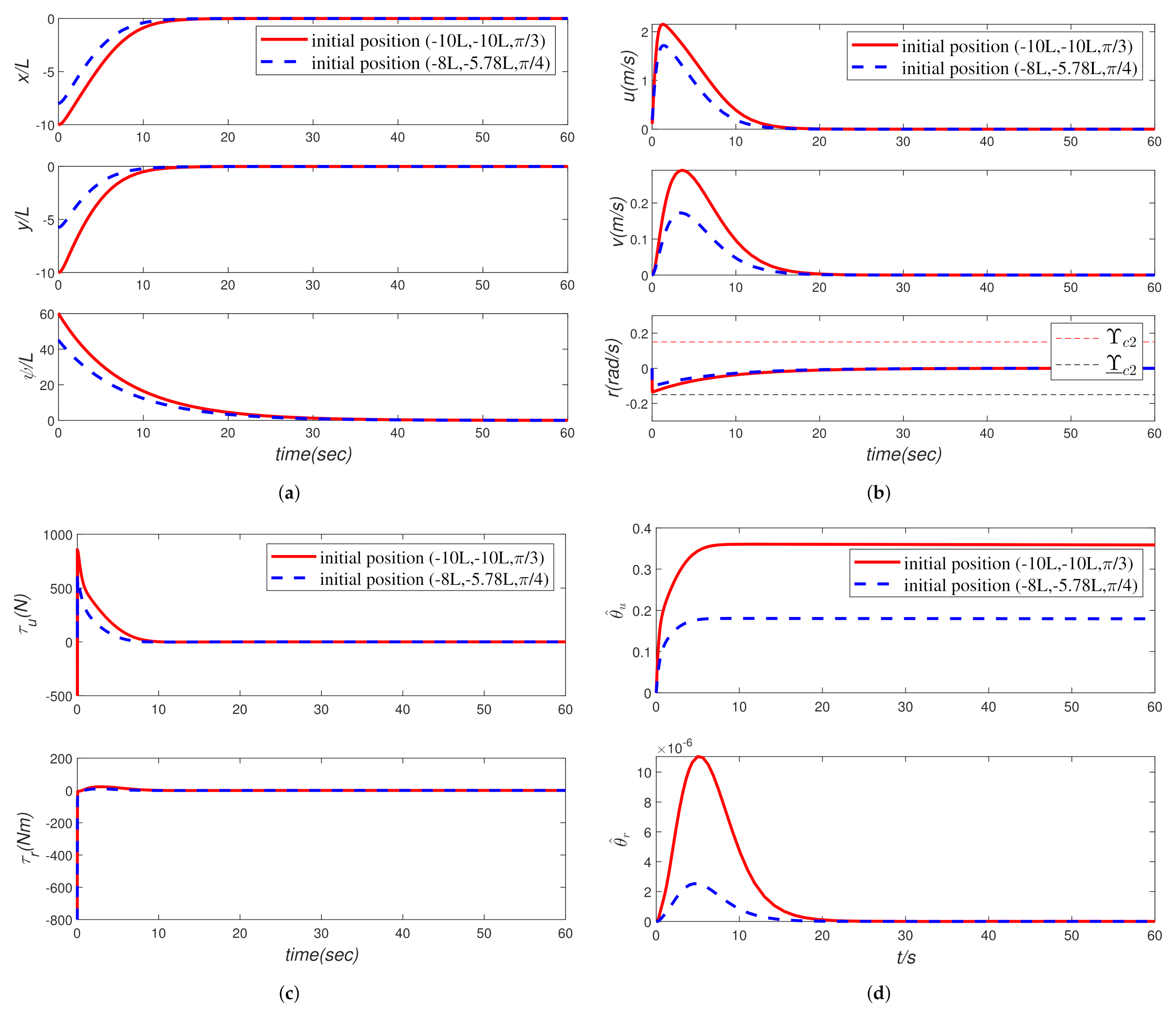
Figure 5 and
Figure 6 show the simulation results. It can be seen that the berthing task is successful with the new initial position.
Figure 7a shows that the lateral position reaches the desired position
x = 0 at 15.58 s, and the longitudinal position reaches the desired position
y = 0 at 14.59 s.
Figure 7b illustrations that the yaw rate does not exceed the limitation.
Figure 7c shows the curves change of control force and control force moment of the vessel with new initial states. It can be seen from the portrait that the surge control force with new initial states increases from −1.731 N to 609.3 N and then gradually stabilizes at 0 N in 10.1 s. The yaw control force moment changes from −816.8 Nm to 9.614 Nm within around 2.7 s and gradually decreases to 0 Nm at 9.4 s.
Figure 7d shows that the adaptive control schemes are all bounded and stable, which proves the effectiveness and practicability of the control scheme designed in this paper.
We clearly illustrate the effectiveness of the proposed control rate in
Table 1.
6. Conclusions
The BLF-based auto-berthing control scheme has been proposed for an underactuated vessel system with 3-DOF considering model uncertain dynamics and yaw rate limitation. The control design applies a differential homeomorphism transformation approach to convert the vessel to a cascade form to solve the underactuated problem. An auto-berthing control scheme is derived based on the backstepping framework, combining BLF, RBF, MLP, and DSC methods. By applying RBF, the uncertain factors affected by the low speed, shallow water, and quay–wall effects are efficiently approximated. Furthermore, a DSC filter is constructed to avoid the differential explosion, and MLP is adopted to improve calculation efficiency. Compared with the auto-berthing control scheme without considering BLF, this method successfully stints the yaw rate in a relatively small range. The Lyapunov-based theoretical analysis indicates that all signals under the proposed auto berthing control scheme are bounded.
However, the proposed method does not solve the problem of the general applicability of the port, and it can only realize automatic berthing from a specific location. In addition, this study does not consider input nonlinearities that may lead to input saturation, hysteresis, dead zones, the effect of communication loads on the system, sway-yaw coupling of vessel model, and tests on actual vessels. The above aspects will be considered in the automatic berthing control design in the future.


