Figure 1.
Suboff geometry.
Figure 1.
Suboff geometry.
Figure 2.
Computational mesh. (a)-around the hull extremities; (b)-side view of the mesh clustering; (c)-top view of the mesh clustering; (d)-cross view from the aft region; (e)-cross view in the midsection.
Figure 2.
Computational mesh. (a)-around the hull extremities; (b)-side view of the mesh clustering; (c)-top view of the mesh clustering; (d)-cross view from the aft region; (e)-cross view in the midsection.
Figure 3.
Grid convergence test performed for the (G
1–G
4) meshes. (
a)-total resistance measured (EFD) [
53,
60] and computed (CFD); (
b)-absolute computational errors.
Figure 3.
Grid convergence test performed for the (G
1–G
4) meshes. (
a)-total resistance measured (EFD) [
53,
60] and computed (CFD); (
b)-absolute computational errors.
Figure 4.
Time histories of the resistance computed on the finest mesh for three advancing speeds.
Figure 4.
Time histories of the resistance computed on the finest mesh for three advancing speeds.
Figure 5.
Comparison between the experimental data [
60] and the numerical solutions computed by using different turbulence models on the finest mesh (
a)-total resistance measured (EFD) and computed (CFD); (
b)-absolute computational errors.
Figure 5.
Comparison between the experimental data [
60] and the numerical solutions computed by using different turbulence models on the finest mesh (
a)-total resistance measured (EFD) and computed (CFD); (
b)-absolute computational errors.
Figure 6.
Time step convergence test. (
a)-total resistance measured (EFD) [
60] and computed (CFD); (
b)-absolute computational errors.
Figure 6.
Time step convergence test. (
a)-total resistance measured (EFD) [
60] and computed (CFD); (
b)-absolute computational errors.
Figure 7.
Absolute errors in the grid convergence test for the static drift computations: (a)-; (b)-.
Figure 7.
Absolute errors in the grid convergence test for the static drift computations: (a)-; (b)-.
Figure 8.
Absolute errors in the grid convergence test for the static drift computations: (a)-; (b)-.
Figure 8.
Absolute errors in the grid convergence test for the static drift computations: (a)-; (b)-.
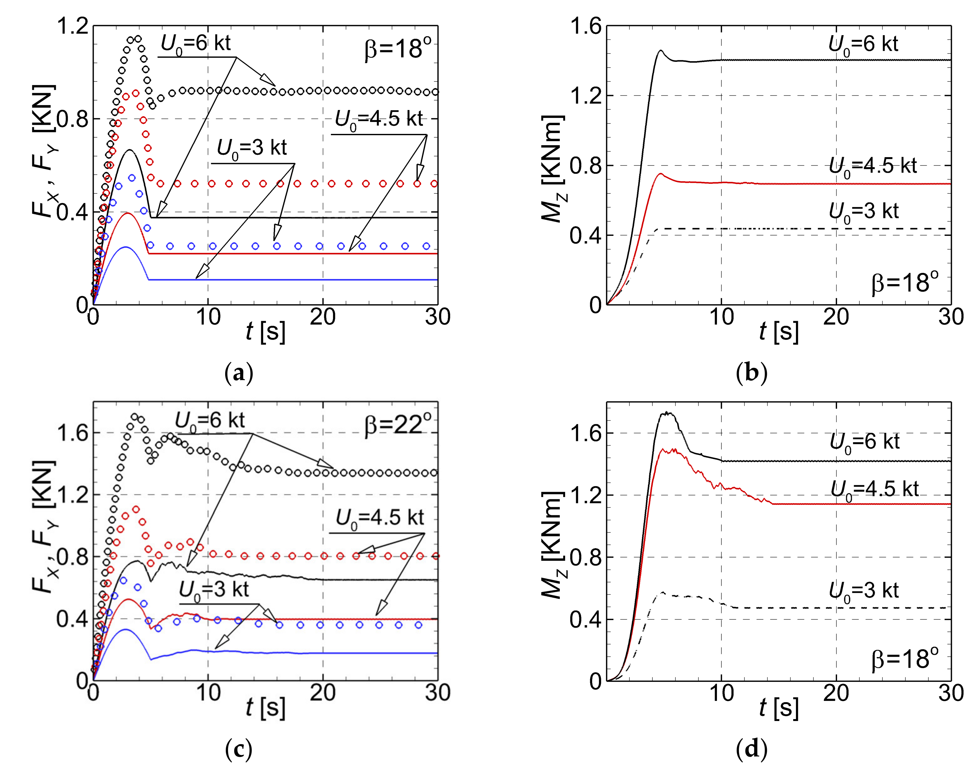
Figure 9.
Time histories of the streamwise and lateral forces and yaw moments computed for three advancing speeds computed for the largest incidence angles: (a)-streamwise and lateral forces in case, (b)-yaw moment in case, (c)-streamwise and lateral forces in case, (d)-yaw moment in case.
Figure 9.
Time histories of the streamwise and lateral forces and yaw moments computed for three advancing speeds computed for the largest incidence angles: (a)-streamwise and lateral forces in case, (b)-yaw moment in case, (c)-streamwise and lateral forces in case, (d)-yaw moment in case.
Figure 10.
Detailed time histories of the streamwise and lateral forces and yaw moments computed for: (a)- case, (b)- case.
Figure 10.
Detailed time histories of the streamwise and lateral forces and yaw moments computed for: (a)- case, (b)- case.
Figure 11.
Instant streamwise non-dimensional velocity (a) and vorticity (b) contours computed at by using the DES-SST turbulence model for.
Figure 11.
Instant streamwise non-dimensional velocity (a) and vorticity (b) contours computed at by using the DES-SST turbulence model for.
Figure 12.
Instant streamwise non-dimensional velocity (a) and vorticity (b) contours computed at by using the DES-SST turbulence model for.
Figure 12.
Instant streamwise non-dimensional velocity (a) and vorticity (b) contours computed at by using the DES-SST turbulence model for.
Figure 13.
Instant streamwise non-dimensional velocity (a) and vorticity (b) contours computed at by using the DES-SST turbulence model for.
Figure 13.
Instant streamwise non-dimensional velocity (a) and vorticity (b) contours computed at by using the DES-SST turbulence model for.
Figure 14.
Wake structure computed for by using the SST turbulence model: (a)—, (b)—, (c)—.
Figure 14.
Wake structure computed for by using the SST turbulence model: (a)—, (b)—, (c)—.
Figure 15.
Time-averaged and instant velocity profiles through the bridge-tip vortex core center computed for
at
knots (
top),
knots (
middle) and
knots (
down) in the transverse directions at three different cross planes, where the vortex core centers from IDDES, DES, RANS, and experimental PIV data [
60] are aligned. Left column:
; middle:
; right column:
.
Figure 16.
Time-averaged and instant velocity profiles through the bridge-tip vortex core centre computed for
at
knots in the transverse directions at three different cross planes, where the vortex core centers from IDDES, DES, RANS and experimental PIV data [
60] are aligned: (
a)-
; (
b)-
; (
c)-
.
Figure 17.
Cross section distribution of instant vorticity and velocity vectors computed for at by using IDDES turbulence model: (a)- (b)-, (c)-.
Figure 17.
Cross section distribution of instant vorticity and velocity vectors computed for at by using IDDES turbulence model: (a)- (b)-, (c)-.
Figure 18.
Instantaneous bridge-tip vortex trajectories computed for at by using IDDES turbulence model: (a)- (b)-.
Figure 18.
Instantaneous bridge-tip vortex trajectories computed for at by using IDDES turbulence model: (a)- (b)-.
Figure 19.
Non-dimensional instant streamwise velocity and vorticity contours computed for at: (a)-non-dimensional streamwise velocity, (b)-vorticity.
Figure 19.
Non-dimensional instant streamwise velocity and vorticity contours computed for at: (a)-non-dimensional streamwise velocity, (b)-vorticity.
Figure 20.
Comparison between the mean non-dimensional pressure fields on the hull computed for at : (a)-, (b)-, (c)-, (d)-.
Figure 20.
Comparison between the mean non-dimensional pressure fields on the hull computed for at : (a)-, (b)-, (c)-, (d)-.
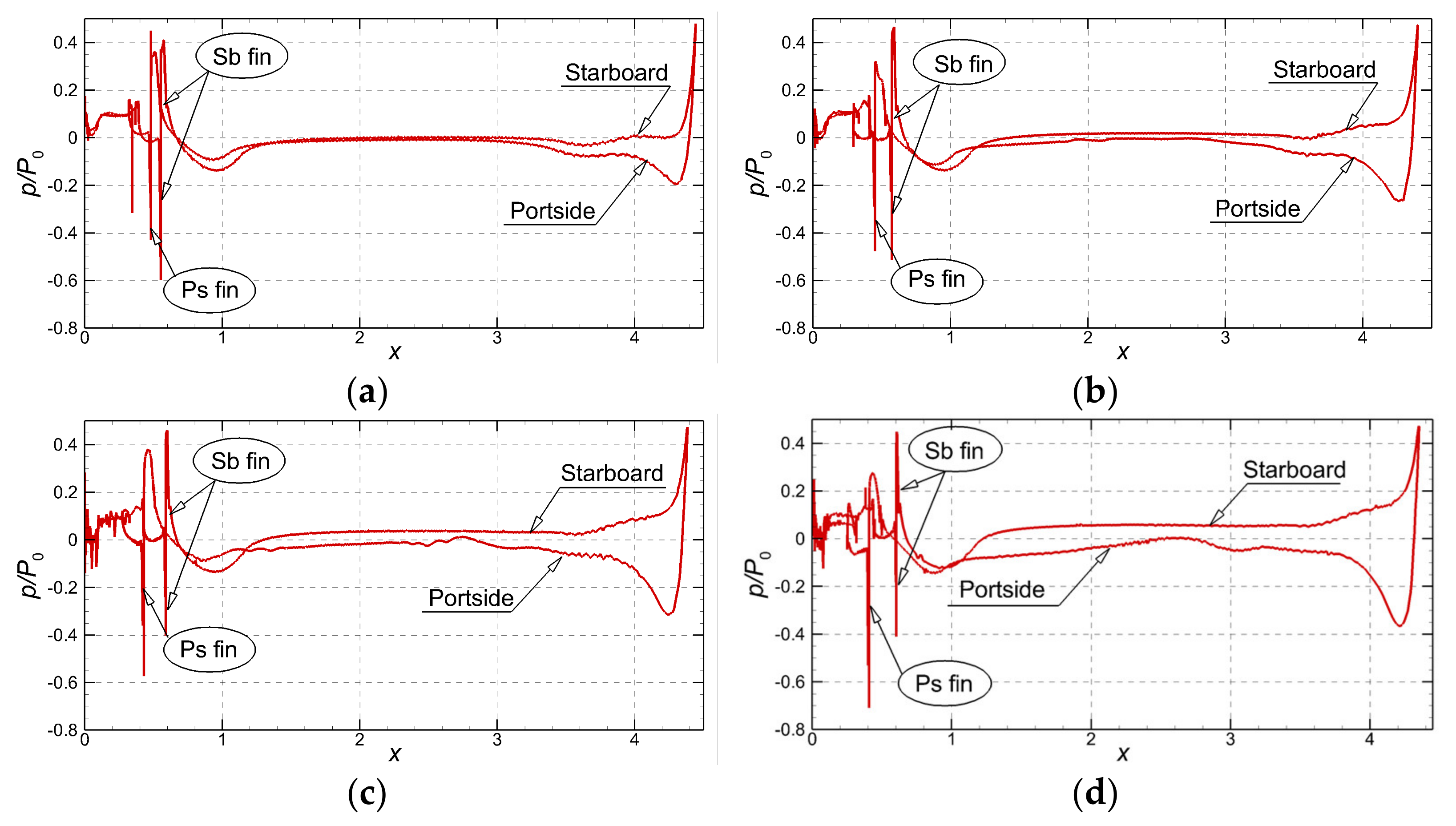
Figure 21.
Comparison between the mean pressures on the Suboff hull computed for at (a)-, (b)-, (c)-, and (d)-.
Figure 21.
Comparison between the mean pressures on the Suboff hull computed for at (a)-, (b)-, (c)-, and (d)-.
Figure 22.
Comparison between the non-dimensional mean pressure fields computed at for at (a)-, (b)-, (c)-, (d)-.
Figure 22.
Comparison between the non-dimensional mean pressure fields computed at for at (a)-, (b)-, (c)-, (d)-.
Figure 23.
Vortex formation mechanisms for (a)- SST model, (b)-DES model, (c)-IDDES model.
Figure 23.
Vortex formation mechanisms for (a)- SST model, (b)-DES model, (c)-IDDES model.
Figure 24.
Vorticity contours computed for at s. by using: (a)- SST turbulence model, (b)-IDDES turbulence model.
Figure 24.
Vorticity contours computed for at s. by using: (a)- SST turbulence model, (b)-IDDES turbulence model.
Figure 25.
Details of wake vorticity contours computed for at s. by using: (a)- SST turbulence model, (b)-IDDES turbulence model.
Figure 25.
Details of wake vorticity contours computed for at s. by using: (a)- SST turbulence model, (b)-IDDES turbulence model.
Figure 26.
Instant isosurfaces of the second invariant of velocity gradient () colored by helicity and computed for at by using the IDDES turbulence model: (a)-, (b)-, (c)-, and (d)-.
Figure 26.
Instant isosurfaces of the second invariant of velocity gradient () colored by helicity and computed for at by using the IDDES turbulence model: (a)-, (b)-, (c)-, and (d)-.
Table 1.
Main particulars of the DARPA Suboff hull.
Table 1.
Main particulars of the DARPA Suboff hull.
| Main Particulars | Symbol | Units | |
|---|
| Length | | m | 4.356 |
| Diameter | | m | 0.508 |
| Wetted surface | | m2 | 6.339 |
| Displacement | | m3 | 0.706 |
| Center of mass | | m | (2.345, 0.000, 0.002) |
Table 2.
Computational grids generated for the grid convergence study—hull in straight run.
Table 2.
Computational grids generated for the grid convergence study—hull in straight run.
| | G1 | G2 | G3 | G4 |
|---|
| Number of cells | 8.01·106 | 1.65·107 | 3.19·107 | 6.41·107 |
| 2.06 | 1.93 | 2.01 |
| 2 |
Table 3.
Grid convergence test for the DARPA Suboff hull. Computations in straight run.
Table 3.
Grid convergence test for the DARPA Suboff hull. Computations in straight run.
| U0 | EFD [60] | CFD |
|---|
| G1 | G2 | G3 | G4 |
|---|
| [knots] | N | R [N] | | | R [N] | | | R [N] | | | R [N] | | |
|---|
| 3 | 40.920 | 39.3118 | 4.09 | 39.6638 | 3.17 | 41.8407 | 2.20 | 41.6975 | 1.86 |
| 3.5 | 45.151 | 43.8045 | 3.07 | 44.0990 | 2.39 | 46.0967 | 2.05 | 45.9462 | 1.73 |
| 4 | 52.014 | 50.5589 | 2.88 | 50.8765 | 2.24 | 53.0340 | 1.92 | 52.8679 | 1.62 |
| 4.5 | 63.222 | 61.5700 | 2.68 | 61.9310 | 2.08 | 64.3974 | 1.83 | 64.2028 | 1.53 |
| 5 | 76.013 | 74.1174 | 2.56 | 74.5315 | 1.99 | 77.3582 | 1.74 | 77.1315 | 1.45 |
| 5.5 | 90.116 | 88.1816 | 2.19 | 88.5511 | 1.77 | 91.5337 | 1.55 | 91.2634 | 1.26 |
| 6 | 105.241 | 103.209 | 1.97 | 103.598 | 1.59 | 106.640 | 1.31 | 106.377 | 1.07 |
Table 4.
Verification for the turbulence models used to simulate the flow on the finest mesh.
Table 4.
Verification for the turbulence models used to simulate the flow on the finest mesh.
| EFD [60] | CFD |
|---|
| DES SST | IDDES SST |
|---|
| [knots] | [N] | [N] | |ε| [%] | [N] | |ε| [%] | [N] | |ε| [%] |
|---|
| 3 | 40.921 | 39.6842 | 3.02 | 39.8274 | 2.67 | 41.69748 | 1.86 |
| 3.5 | 45.152 | 43.9987 | 2.55 | 44.1793 | 2.15 | 45.94615 | 1.73 |
| 4 | 52.012 | 50.8086 | 2.31 | 51.0270 | 1.89 | 52.86788 | 1.62 |
| 4.5 | 63.221 | 61.8544 | 2.16 | 62.0694 | 1.82 | 64.20278 | 1.53 |
| 5 | 76.013 | 74.4366 | 2.07 | 74.6798 | 1.75 | 77.13149 | 1.45 |
| 5.5 | 90.114 | 88.3619 | 1.94 | 88.5871 | 1.69 | 91.26341 | 1.26 |
| 6 | 105.241 | 103.3983 | 1.75 | 103.6509 | 1.51 | 106.3766 | 1.07 |
Table 5.
Time step convergence test for the DARPA Suboff hull. Computations in the straight run case, IDDES turbulence model.
Table 5.
Time step convergence test for the DARPA Suboff hull. Computations in the straight run case, IDDES turbulence model.
| EFD | CFD |
|---|
| | | |
|---|
| knots | | | |ε|[%] | | |ε|[%] | | |ε|[%] | | |ε|[%] |
|---|
| 3 | 40.92 | 41.6975 | 1.86 | 39.7685 | 2.90 | 39.2749 | 4.19 | 36.6516 | 11.65 |
| 4 | 52.014 | 52.8679 | 1.62 | 50.7301 | 2.53 | 50.1818 | 3.65 | 47.2303 | 10.13 |
| 5 | 76.013 | 77.1315 | 1.45 | 74.3298 | 2.26 | 73.6104 | 3.26 | 69.7012 | 9.06 |
| 6 | 105.241 | 106.377 | 1.07 | 103.512 | 1.67 | 102.767 | 2.41 | 98.6459 | 6.69 |
Table 6.
Verification and validation for the total resistance in the straight run case.
Table 6.
Verification and validation for the total resistance in the straight run case.
| Parameter | Speed
[knots] | | | | | | |
|---|
| [N] | 3 | 2 | 0.34 | 1.236 | 1.921 | 1.78 | 2.619 |
| 3.5 | 0.32 | 1.156 | 1.872 | 2.583 |
| 4 | 0.30 | 1.197 | 1.816 | 1.543 |
| 4.5 | 0.30 | 1.264 | 1.805 | 2.535 |
| 5 | 0.29 | 1.208 | 1.713 | 2.470 |
| 5.5 | 0.29 | 1.123 | 1.711 | 2.469 |
| 6 | 0.24 | 1.152 | 1.704 | 2.464 |
Table 7.
Meshes generated for the grid convergence study. Drift angle
Table 7.
Meshes generated for the grid convergence study. Drift angle
| | G1 | G2 | G3 | G4 |
|---|
| Number of cells | 8.248·106 | 1.666·107 | 3.285·107 | 6.58·107 |
| 2.02 | 1.975 | 2.00 |
| 1.992 |
Table 8.
Grid convergence study. Run at the drift angle
Table 8.
Grid convergence study. Run at the drift angle
| EFD | CFD |
|---|
| G1 | G2 | G3 | G4 |
|---|
| knots | [N] | [N] | | [N] | | [N] | | [N] | |
|---|
| 3 | 119.921 | 116.035 | 3.35 | 116.997 | 2.50 | 117.434 | 2.12 | 117.695 | 1.89 |
| 4.5 | 269.971 | 262.408 | 2.88 | 264.287 | 2.15 | 265.139 | 1.82 | 265.648 | 1.63 |
| 6 | 483.837 | 473.421 | 2.20 | 476.021 | 1.64 | 477.197 | 1.39 | 477.900 | 1.24 |
| | [Nm] | [Nm] | || | [Nm] | || | [Nm] | || | [Nm] | || |
| 3 | 188.199 | 180.406 | 4.32 | 181.553 | 3.66 | 182.536 | 3.10 | 193.412 | 2.77 |
| 4.5 | 426.614 | 411.904 | 3.57 | 414.082 | 3.03 | 415.946 | 2.56 | 436.383 | 2.29 |
| 6 | 733.504 | 713.0431 | 2.87 | 716.090 | 2.43 | 718.693 | 2.06 | 747.000 | 1.84 |
Table 9.
Meshes generated for the grid convergence study. Drift angle
Table 9.
Meshes generated for the grid convergence study. Drift angle
| | G1 | G2 | G3 | G4 |
|---|
| Number of cells | 8.248·106 | 1.666·107 | 3.285·107 | 6.58·107 |
| 2.02 | 1.975 | 2.00 |
| 1.992 |
Table 10.
Grid convergence study. Run at the drift angle
Table 10.
Grid convergence study. Run at the drift angle
| EFD | CFD |
|---|
| G1 | G2 | G3 | G4 |
|---|
| knots | [N] | [N] | | [N] | | [N] | | [N] | |
|---|
| 3 | 119.921 | 116.035 | 3.35 | 116.997 | 2.50 | 117.434 | 2.12 | 117.695 | 1.89 |
| 4.5 | 269.971 | 262.408 | 2.88 | 264.287 | 2.15 | 265.139 | 1.82 | 265.648 | 1.63 |
| 6 | 483.837 | 473.421 | 2.20 | 476.021 | 1.64 | 477.197 | 1.39 | 477.900 | 1.24 |
| | [Nm] | [Nm] | || | [Nm] | || | [Nm] | || | [Nm] | || |
| 3 | 188.199 | 180.406 | 4.32 | 181.553 | 3.66 | 182.536 | 3.10 | 193.412 | 2.77 |
| 4.5 | 426.614 | 411.904 | 3.57 | 414.082 | 3.03 | 415.946 | 2.56 | 436.383 | 2.29 |
| 6 | 733.504 | 713.0431 | 2.87 | 716.090 | 2.43 | 718.693 | 2.06 | 747.000 | 1.84 |
Table 11.
Meshes generated for the grid convergence study. Drift angle
Table 11.
Meshes generated for the grid convergence study. Drift angle
| | G1 | G2 | G3 | G4 |
|---|
| Number of cells | 8.87·106 | 1.78·107 | 3.55·107 | 7.17·107 |
| 2.01 | 1.99 | 2.02 |
| 2.007 |
Table 12.
Grid convergence study. Run at the drift angle
Table 12.
Grid convergence study. Run at the drift angle
| EFD | CFD |
|---|
| G1 | G2 | G3 | G4 |
|---|
| knots | [N] | [N] | | [N] | | [N] | | [N] | |
|---|
| 3 | 282.337 | 271.741 | 3.90 | 274.353 | 2.91 | 275.252 | 2.57 | 275.994 | 2.30 |
| 4.5 | 578.714 | 558.180 | 3.68 | 563.251 | 2.75 | 565.556 | 2.33 | 566.937 | 2.08 |
| 6 | 1009.380 | 984.123 | 2.57 | 990.411 | 1.92 | 993.259 | 1.62 | 994.961 | 1.45 |
| | [Nm] | [Nm] | || | [Nm] | || | [Nm] | || | [Nm] | || |
| 3 | 421.923 | 398.436 | 5.89 | 401.848 | 5.00 | 404.786 | 4.23 | 437.872 | 3.78 |
| 4.5 | 910.225 | 868.121 | 4.85 | 874.290 | 4.11 | 879.587 | 3.48 | 938.533 | 3.11 |
| 6 | 1423.98 | 1379.45 | 3.23 | 1386.066 | 2.74 | 1391.72 | 2.32 | 1453.46 | 2.07 |
Table 13.
Meshes generated for the grid convergence study. Drift angle
Table 13.
Meshes generated for the grid convergence study. Drift angle
| | G1 | G2 | G3 | G4 |
|---|
| Number of cells | 9.08·106 | 1.797·107 | 3.666·107 | 7.48·107 |
| 1.98 | 2.04 | 2.04 |
| 2.02 |
Table 14.
Grid convergence study. Run at the drift angle
Table 14.
Grid convergence study. Run at the drift angle
| EFD | CFD |
|---|
| G1 | G2 | G3 | G4 |
|---|
| knots | [N] | [N] | | [N] | | [N] | | [N] | |
|---|
| 3 | 410.937 | 394.852 | 4.07 | 398.813 | 3.04 | 401.043 | 2.47 | 402.080 | 2.20 |
| 4.5 | 915.261 | 884.359 | 3.49 | 892.001 | 2.61 | 895.472 | 2.21 | 897.551 | 1.97 |
| 6 | 1509.28 | 1471.85 | 2.54 | 1481.17 | 1.90 | 1485.39 | 1.61 | 1487.92 | 1.44 |
| | [Nm] | [Nm] | || | [Nm] | || | [Nm] | || | [Nm] | || |
| 3 | 456.114 | 428.641 | 6.41 | 432.616 | 5.43 | 436.043 | 4.60 | 474.861 | 4.11 |
| 4.5 | 1105.82 | 1049.68 | 5.35 | 1057.87 | 4.53 | 1064.94 | 3.84 | 1143.75 | 3.43 |
| 6 | 1878.83 | 1814.86 | 3.52 | 1824.34 | 2.99 | 1832.44 | 2.53 | 1921.29 | 2.26 |
Table 15.
Verification and validation of the total resistance computed in the drift angle case.
Table 15.
Verification and validation of the total resistance computed in the drift angle case.
| Parameter | Speed
[knots] | | | | | | |
|---|
| [N] | 3 | 2.02 | 0.27 | 1.252 | 1.971 | 1.92 | 2.751 |
| 4.5 | 0.24 | 1.211 | 1.814 | 2.641 |
| 6 | 0.17 | 1.158 | 1.722 | 2.597 |
Table 16.
Verification and validation for the yaw moment computed for drift angle case.
Table 16.
Verification and validation for the yaw moment computed for drift angle case.
| Parameter | Speed
[knots] | | | | | | |
|---|
| [Nm] | 3 | 2.02 | 0.89 | 1.252 | 1.618 | 1.85 | 2.458 |
| 4.5 | 0.54 | 1.211 | 1.507 | 2.386 |
| 6 | 0.05 | 1.158 | 1.404 | 2.322 |


