Wave Transformation behind a Breakwater in Jukbyeon Port, Korea—A Comparison of TOMAWAC and ARTEMIS of the TELEMAC System

Abstract

Severe shoreline erosions are commonly observed due to the side effects of breakwaters constructed to protect the habitat. These breakwaters can cause wave energy differences behind the structure due to diffraction, inducing longshore sediment transport and resulting in shoreline changes. Therefore, it is essential to correctly simulate the effect of wave transformation in the lee side of structures, but such studies reporting performance of models in the field have been relatively rare. In this study, two wave models of the TELEMAC system were used to investigate the accuracy of modeling the wave transformation effect in a lee area of a breakwater built to secure the harbor’s tranquility, near Jukbyeon Port in Korea, through comparisons with field observations. Two cases of wave conditions with different wave heights and directions were tested. In both cases, the TEL EMAC–ARTEMIS model had lower errors than TELEMAC–TOMAWAC at the onshore wave location, confirming that the phase-resolving ARTEMIS showed better performance in simulating the wave transformation than the phase-averaged TOMAWAC, as expected. However, ARTEMIS had slightly higher errors than TOMAWAC at the offshore location, probably due to the interference by reflected waves from the complex coastlines formed by the different coastal structures. The results also provide various implications learned from the numerical experiments, which can be usefully applied to engineering aspects, such as for the estimation of harbor tranquility.

1. Introduction

One serious problem that many sandy beaches are currently facing is coastal erosion, as it can cause economic and environmental damage to habitats and nearby communities. The threat of erosion has been increasing due to natural causes, such as climate change [1,2]. However, human interventions such as coastal structures can also lead to side effects of erosional damages [3]. In some extreme cases, the coastal structures constructed to protect the sand on the beach can even worsen the erosional process. For example, Figure 1 shows that a set of coastal structures, headland breakwaters (HBs), and submerged breakwaters (SBs), were built to protect the sand at the study site. However, the erosion became more severe due to the presence of these breakwaters, which was unexpected when they were initially designed. The main reason for the erosion was the wave transformation—diffraction and refraction—in the lee area of the structures [4]. When shadow zones formed in the lee area of the HBs, the diffracted waves produced gradients in the wave energy distribution to move sand toward the HBs, causing erosion in the shoreline, in-between the HBs. To understand and precisely predict the sediment’s motions and erosional process around such coastal structures, it is therefore essential to increase the modeling accuracy to simulate the effect of the wave transformation caused by the presence of these structures.

In this study, the effect of wave transformation in a two-dimensional field behind a breakwater (BW) was examined through comparisons of numerical models developed for wave propagation in coastal areas. There are numerous studies that have investigated wave transformation behind BWs using numerical models [5,6,7,8]. However, numerical experiments in a real sea environment have been relatively rare, according to the authors’ knowledge. In the present study, the simulation results of two wave models were compared with observational data to analyze the models’ performance in terms of the implementation of the refraction and diffraction effect behind a BW.

Behind a BW, the combined effects of wave shoaling, refraction, and diffraction would lead to the transformation of the propagating waves, modifying the waves’ heights and directions [9], leading to a reduction in the wave energy, which contributes to enhancing the tranquility inside the port/harbor [10]. However, unexpected side effects such as coastal erosion could also occur in the shadow zone behind the BW due to the gradient of the wave energy generated along the coast, caused by the wave transformation [4]. Therefore, an accurate estimation of the effect of the transformation of the propagating waves is necessary not only to secure harbor tranquility but also to protect the coastal areas from anthropogenic disasters by coastal structures.

For this purpose, area models in which wave, current, sediment, and morphology modules are combined [11,12] have been widely used for lab experiments [13,14] or for simulations in the field [15,16]. These process-based models are computationally efficient in simulating the wave transformation and the consequent morphological changes in the lee area of BW or similar coastal structures. However, their accuracy has been questioned as the wave modules are usually based on the phase-averaged wave models that solve the wave action balance equation. These phase-averaged models may not properly calculate the effects of wave diffraction, reflection, and run-up in the nearshore [8].

On the other hand, the phase-resolving wave models that solve mild-slope [17] or Boussinesq equations [18] could have better performance in resolving the wave transformation processes. One of the shortcomings of these phase-resolving models is the high computational cost; thus, their applications for long-term predictions in wide coastal regions have been limited [19]. However, the coupling of phase-resolving wave models with sediment transport and morphology modules has been recently practiced for their application in various processes around coastal structures, such as emerged detached BW [20], submerged detached BW [21,22], groyne [8], or for the simulation of ship-wake induced morphological changes [23]. Specifically, Karambas and Samaras [21] tested their model not only with the lab data, but they also applied it in the field where multiple coastal structures had been established.

These previous studies were focused on simulating wave-induced currents and morphological changes around the coastal structures. The present study focused on simulating the effect of wave transformation, specifically the diffraction/refraction of the waves that propagated to the port behind a BW, which is an important process to secure a port’s tranquility but still limited when using numerical models.

For this, we employed two different wave propagation models: the phase-resolving model based on the mild-slope equation, TELEMAC–ARTEMIS [17]; the phase-averaged model based on the wave action balance equation, TELEMAC–TOMAWAC [24]. These two wave models are part of the TELEMAC system [24], which is, a set of software for the numerical modeling of hydrodynamics, waves, sediment, and morphology. The purpose of this study was then to examine the performance of these models in estimating the effect of wave transformation around a BW constructed to secure harbor tranquility in the Jukbyeon Port in Korea. This was conducted by comparison with the real-field observation data, which is one of its advantages, as previous studies that tested the wave model performance on transformation (diffraction and refraction) behind the coastal structures by comparisons with the in situ observational data are rare, to the authors knowledge. Previously, the wave transformation effect was examined using only one phase-averaged wave model, TELEMAC–TOMAWAC, by controlling the diffraction mode applied in the lee area of a breakwater to estimate the impact on the coastal erosion that was caused by the gradient of the sediment transport along the shore due to the transformation of the propagating waves in the lee area [4]. In this study, we did not simulate the sediment transport and the consequent shoreline evolution. Instead, we focused on investigating the wave propagation in the lee area of the BW, aiming to compare the effect of the wave transformation between the two models: the phase-averaged and phase-resolving models.

2. Materials and Methods

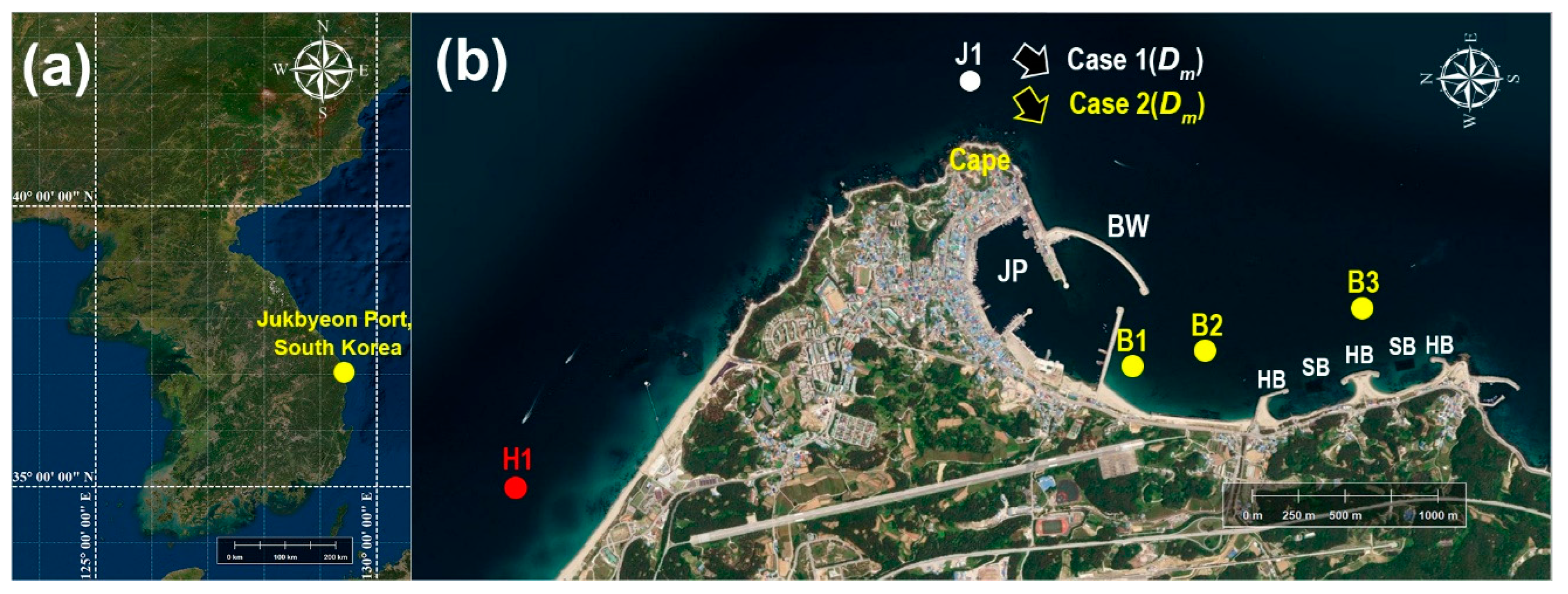
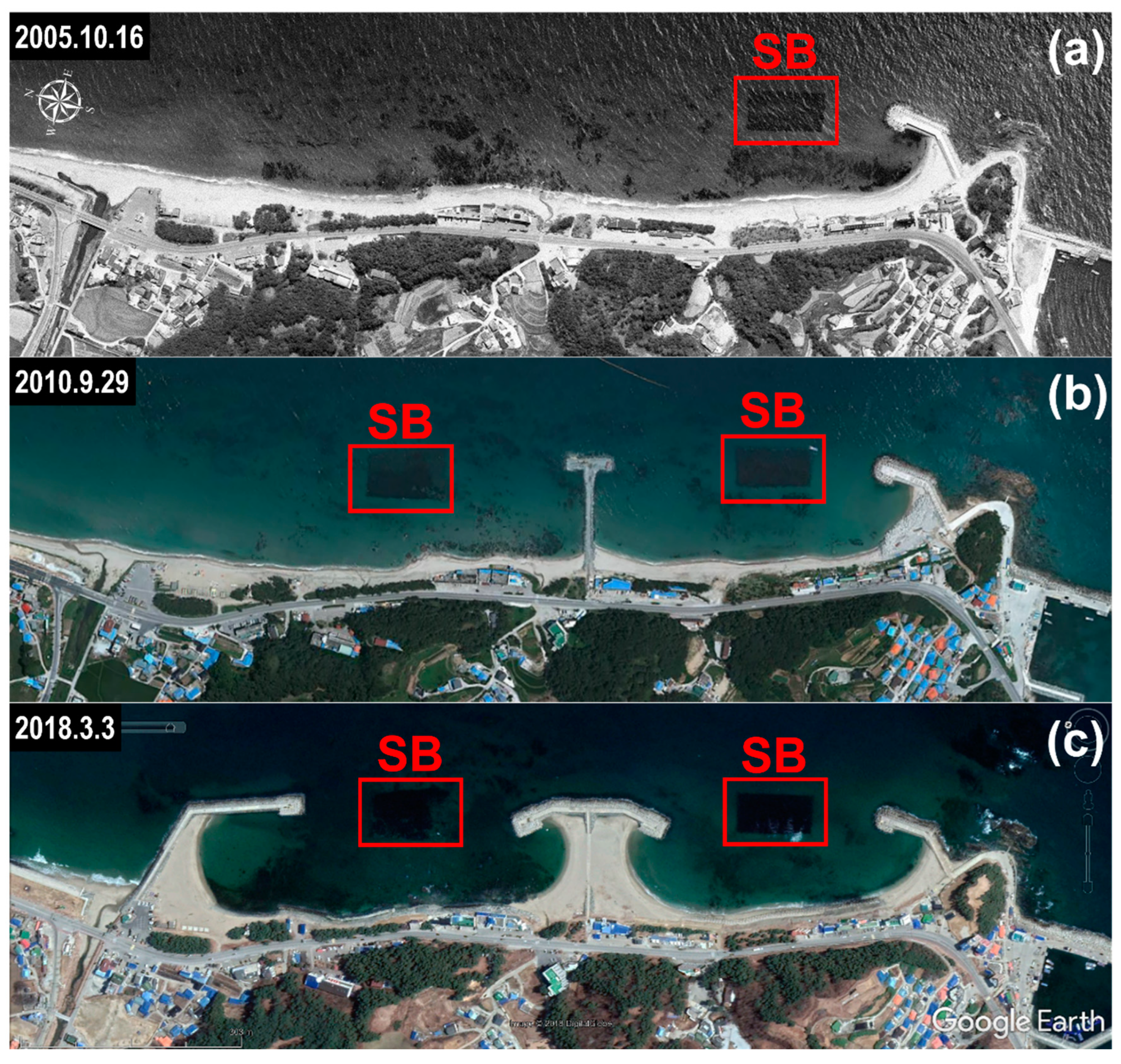
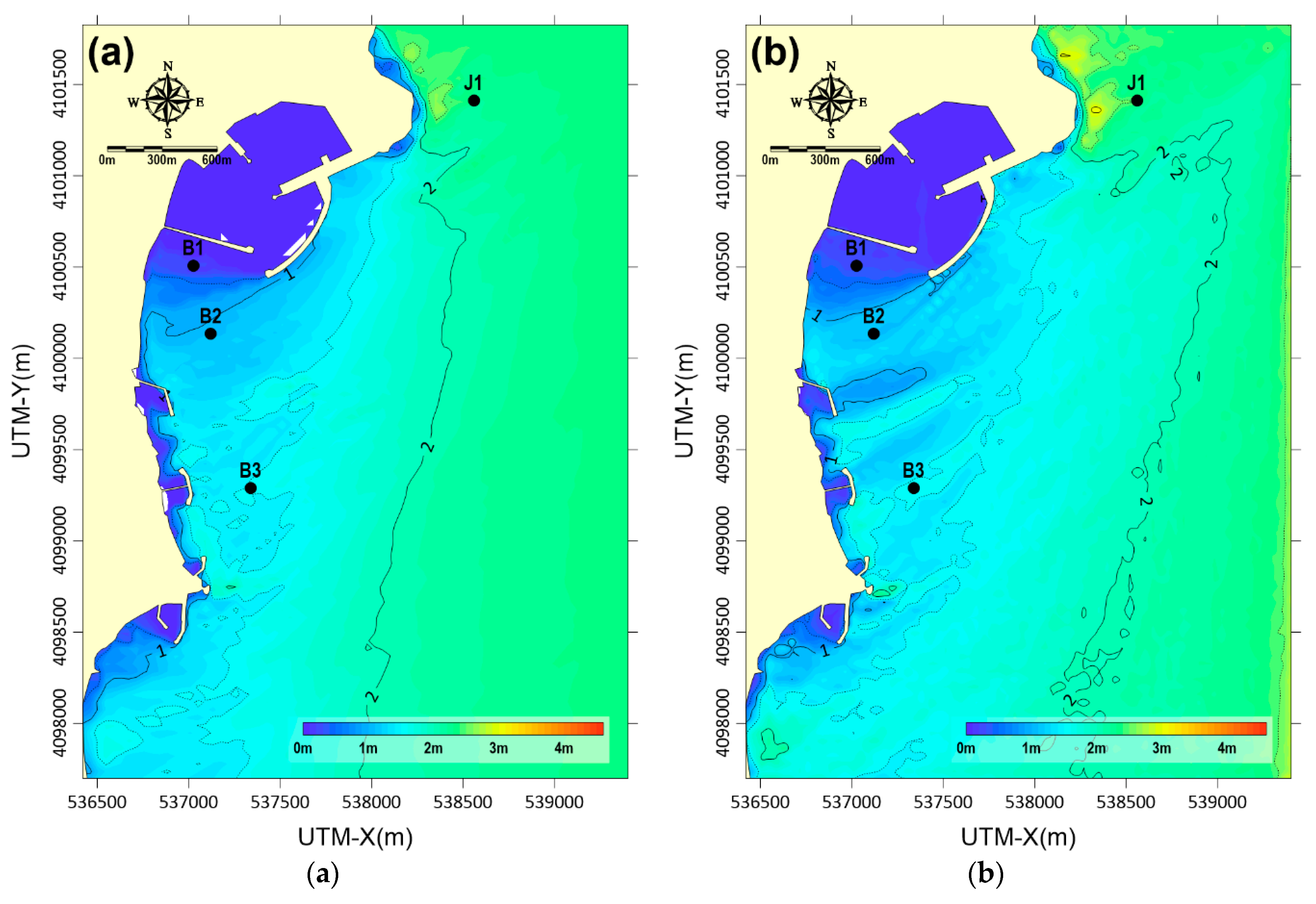
2.1. Study Site

Jukbyeon Port (JP) is located in the middle of the east coast of the Korean Peninsula (Figure 1a). North of the port, a cape was developed from which a breakwater (BW) was constructed in the SE direction. Therefore, the BW could effectively block waves that propagated from the NE and E directions, the primary direction of the propagating waves in this region. In Figure 2, two wave roses are plotted showing the wave conditions in winter and summer in this area. The winter wave rose was based on the measurements from December 2019 to February 2020 in H1, and the summer rose was based on the measurements from June to August 2020. In winter, the wave propagation direction ($D_p$) ranged from NNE to NE, with the majority of the waves approaching in the NE direction, which confirmed the effectiveness of the BW when the waves approached in the represented direction. In summer, the primary wave direction was still NE. However, the waves approached from more diverse directions, as ~30% of the waves were from E and ESE directions. The measured wave height was higher in winter. The significant wave height ($H_s$) which was greater than 1 m was observed to be ~43.7% in winter. In addition, ~13.5% of $H_s$ was greater than 2 m, as they could be categorized as storm waves in this area [25]. In contrast, more than 85.2% of $H_s$ was lower than 1 m in summer. As confirmed from the data in the wave roses, the wave condition is usually rougher in winter in this region, except for the extreme storm waves caused by typhoons that are usually affiliated with the Korean Peninsula in late summer or early autumn.

Although the BW effectively reduced the wave energy inside JP, side effects also occurred due to the shadow zone formed in the lee area of the BW. A shadow zone is an area behind an obstacle, into which the waves can be bent into due to wave diffraction. Because the wave energy gradually decreased in the shadow zone, as the diffracted wave was further propagated behind the obstacle (the BW in this case), the capacity of the sediment movement varied along the shore causing shoreline erosion near the outer edge of the shadow zone, whereas shoreline accretion occurred behind the obstacle [4]. Similar coastal erosion occurred in the beach located in the south of JP in which the coastal structures—a set of headland breakwaters (HBs)—were built to protect the beach from coastal erosion, as shown in Figure 1b. In addition, two submerged breakwaters (SBs) were placed in between the three HBs. The results of the construction of these structures were, however, not successful. In Figure 3, a collection of snapshot pictures shows the beach status throughout the history of these structures. In 2005, only one piece of the HB, a groin, and an SB were built at the southern end of the beach (Figure 3a). This set of structures was effective in conserving the beach sand, as the shoreline was considerably advanced at that time. However, further construction of the structures led to unfavorable results. As shown in Figure 3b,c, the shorelines in 2010 and 2018 had retreated compared to 2005, likely due to the additional structures. In particular, after the set of HB and SB was completed in 2018, the shorelines in between the HB were severely eroded, whereas the sand was moved and accumulated near the HBs that were built perpendicular to the shore. The severe erosions of this beach have brought concerns regarding the coastal protection of this area, which have motivated various experiments and observations in the study site near JP.

2.2. Field Experiment

Considering the wave climate in the study area, where the wave conditions are more energetic in the winter, the field experiment in the present study was conducted for 46 days from 15 December 2019 to 29 January 2020, when the storm waves ($H_s$ > 2 m) frequently attacked the study site. In this period, an AWAC (acoustic wave and current profiler, Nortek, Rud, Norway) was moored in J1, in front of the cape, as shown in Figure 1b, to observe the wave conditions outside the port. At the same time, vector velocimeters by Nortek were moored at the three wave stations of B1, B2, and B3 (Figure 1b). B1 was located just behind the BW outside JP at a depth of 5 m, which had its position within the shadow zone formed behind the BW. Therefore, the waves that reached B1 would be transformed by the diffraction. B2 was located near the border of the shadow zone at a depth of 10 m, considering that the majority of the waves approached in the NE direction in this area, specifically during the time of the field experiment, as shown in Figure 2a. In case of B3, the vector was located outside the shadow zone, ~870 m south of B2 along the coast at a depth of 10 m. The positions of B1, B2, B3, and J1 were determined to observe the wave transformation along the propagation paths toward the port, during the field experiment. It is to be noted that in the lee (shoreward) of B3, the HB and SB were located as shown in Figure 1b, which provided the complex feature of the shorelines, specifically in the lee area of B3.

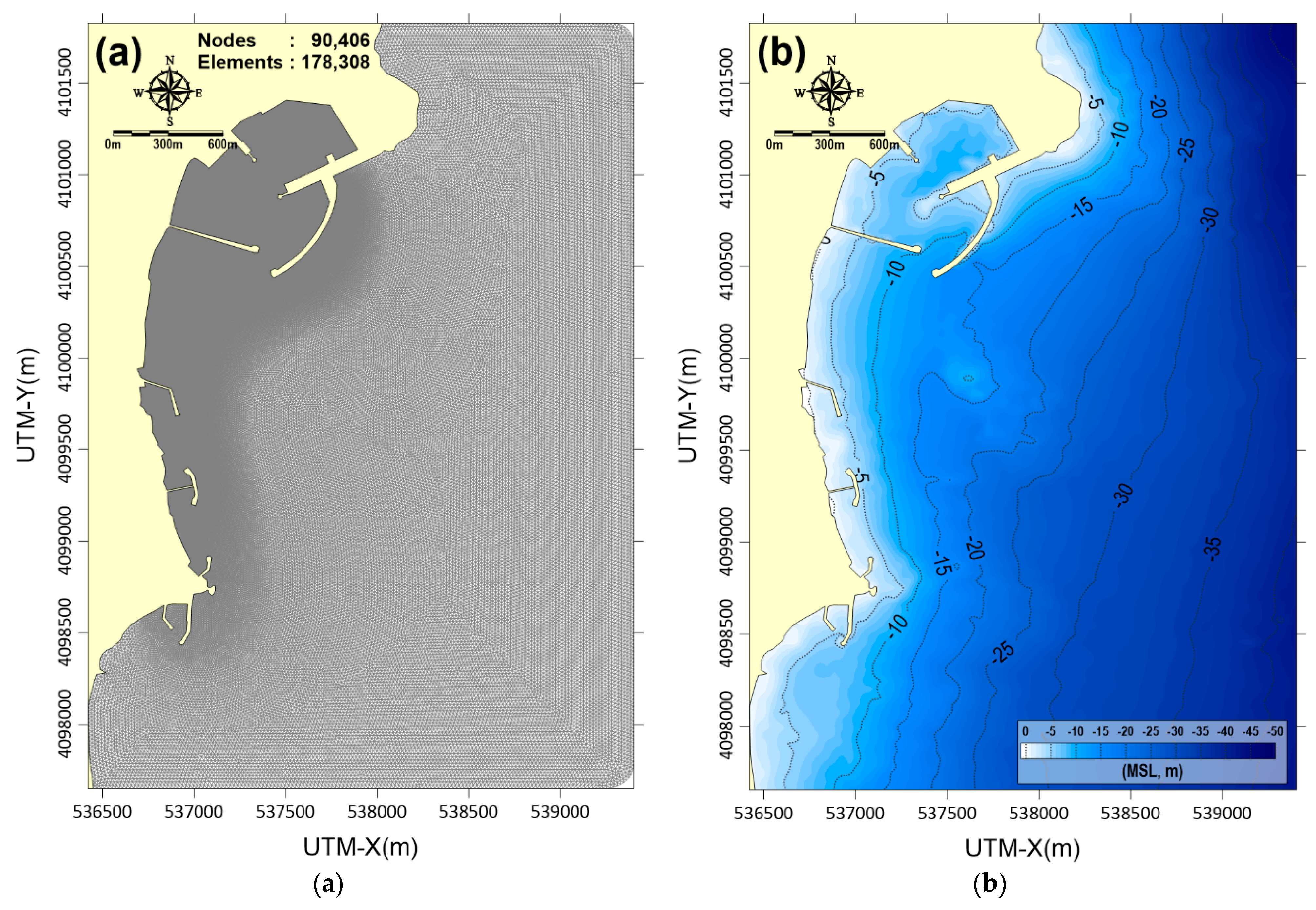
2.3. Numerical Model Experiments

The two wave models employed in this study to simulate wave propagation were TELEMAC–TOMAWAC [26] and TELEMAC–ARTEMIS [17]. Both TOMAWAC and ARTEMIS are wave modules in the TELEMAC system [24]. The TELEMAC system is an integrated suite that consists of modules of solvers for hydrodynamics, waves, sediment, and morphology, and it was developed based on the finite-element method using unstructured grids. TOMAWAC is a phase-averaged wave propagation model in the TELEMAC system, whereas ARTEMIS is a phase-resolving model. In this section, these models are only briefly described, because they are well documented in the listed references. Phase-averaged wave models such as TOMAWAC are based on the spectral action balance equation for wave energy [27]:

$$\frac{\partial N}{\partial t}+\frac{\partial C_{g,x}N}{\partial x}+\frac{\partial C_{g,y}N}{\partial y}+\frac{\partial C_{g,\sigma }N}{\partial \sigma }+\frac{\partial C_{g,\theta }N}{\partial \theta }=\frac{S_{tot}}{\sigma }$$

(1)

where $N$ is the wave action spectral density, $\sigma$ is the intrinsic frequency, $\theta$ is the wave direction, $C_g$ is the group velocity in space ($x$, y, $\sigma$, $\theta$), and $S_{tot}$ is the total source/sink for the wave action. One of the characteristics of TOMAWAC is that this wave module is internally coupled with the hydrodynamic module in the TELEMAC system, so that the interaction between the waves and currents can be modeled by TOMAWAC [28], which is distinguished from other phase-averaged wave models such as SWAN [29].

In TOMAWAC, the effect of the wave diffraction can be considered based on the approximation from the mild-slope equation [30], which suggests that the wavelength could change in the presence of diffraction:

$${\left|k_2\right|}^2=k_1{}^2\left(1+\delta \right)$$

(2)

where $k_1$ and $k_2$ are the wave numbers without/with diffraction, respectively, and $\delta$ is the diffraction parameter given as:

$$\delta =\frac{\nabla ·\left(C{C}_g\nabla a\right)}{k_1{}^{2}C{C}_{g}a}$$

(3)

where $a$ is the wave amplitude, $C$ is the celerity, and $C_g$ is the group velocity. The wave energy propagation speed with diffraction ($C_{gd}$) is given as:

$$C_{gd}=\frac{k_2}{k_1}{C}_g$$

(4)

TELEMAC–ARTEMIS is another wave module in the TELEMAC system, but it is a phase-resolving model that solves the mild-slope equation [31] as:

$$\nabla ·\left(C{C}_g\nabla \varnothing \right)+C{C}_g{k}^2\varnothing =0$$

(5)

where $\varnothing$ is the reduced velocity potential based on the consideration of inviscid, irrotational, and incompressible fluid and for a mildly-varying bottom slope ($\left[\frac{∆\mathrm{h}}{\mathrm{h}}\right]/\left[\frac{\mathrm{h}}{\mathrm{L}}\right]\ll$1). From $\varnothing \left(x,y\right)$ in Equation (5), the total velocity potential $\varnothing \left(x, y, z, t\right)$ can be calculated, and other wave parameters, such as wave amplitude and wave phase, can be derived from $\varnothing \left(x, y, z, t\right)$.

The two wave models were set-up in the same unstructured grid system shown in Figure 4, in which JP and the beach, located south of the port, were included. There were 178,308 elements and 90,406 nodes. The smallest grid size was 5 m near the coastline (Figure 4a). The cell size in the wave propagation direction was ~17 m near the open boundary where the water depth ranged 35–40 m. In the case of Case 2 when $H_s$ was 3.81 m and $T_p$ was 11.72 sec, the mean wavelength was 144.22 m considering a water depth of 35 m. Therefore, 8–9 grids points were used to resolve one wavelength, which provides validation of the model in terms of the grid resolution as phase-resolving wave models typically require a resolution of at least 8–10 grid points per wavelength [32]. However, there could be uncertainties in the ARTEMIS results related to the coarse grid used in this study. The water depths used in the models were calculated from the bathymetry measurements (Figure 4b). The models were run for two different cases (Case 1 and Case 2) that were designed from the observations during the field experiment. For example, the forcing conditions at the models’ open boundaries were taken from the wave data measured in J1 (Figure 1b). In Case 1, the models’ forcing conditions were selected from the wave measurements at 11:00 am on 18 December 2019, when the storm waves with an $H_s$ of 2.36 m and a peak wave period ($T_p$) of 8.93 s affiliated the study site. The peak wave direction ($D_m$) was measured to be 36. 40$°$ as the waves approached from the NNE (clockwise from the north, N = 0$°$ and NE = 45$°$). The boundary conditions for Case 2 were selected from the measurements at 20:00 pm on 8 January 2020, when the severest storm waves attacked the site. The $H_s$ in Case 2 was 3.81 m, and $T_p$ and $D_m$ were measured as 11.72 s and 57.33$°$, respectively, indicating that the waves approached from the NE to ENE in Case 2. These model forcing conditions for the numerical experiments are listed in

Table 1. List of wave parameters used as the forcing (boundary) conditions for both models in the two runs of Case 1 and Case 2. The model input data were determined based on the measurements during the field experiment.

Model Runs	Time of Wave Measurement	${\mathit{H}}_{\mathit{s}}$	${\mathit{T}}_{\mathit{p}}$	${\mathit{D}}_{\mathit{m}}$
Case 1	18 December 2019 11:00 a.m.	2.36 m	8.93 s	36.40$°$
Case 2	8 January 2020 20:00 p.m.	3.81 m	11.72 s	57.33$°$

. The validation of the models’ results was also performed using the observation data measured in B1, B2, and B3 (Figure 1b) by comparing the wave parameters, such as $H_s$ and $D_m$. In the case of TOMAWAC, the results could be directly compared with observations, as they also calculated $H_s$ and $D_m$ from the spectra. For ARTEMIS, the time-dependent fields of the propagating waves were analyzed to estimate these parameters, which is further described in Section 3.2. TOMAWAC was run for 30 min until it reached a stable state. In ARTEMIS, an iteration method was applied to reduce the error that was induced in solving the time independent form of the mild-slope equation, Equation (5).

3. Results

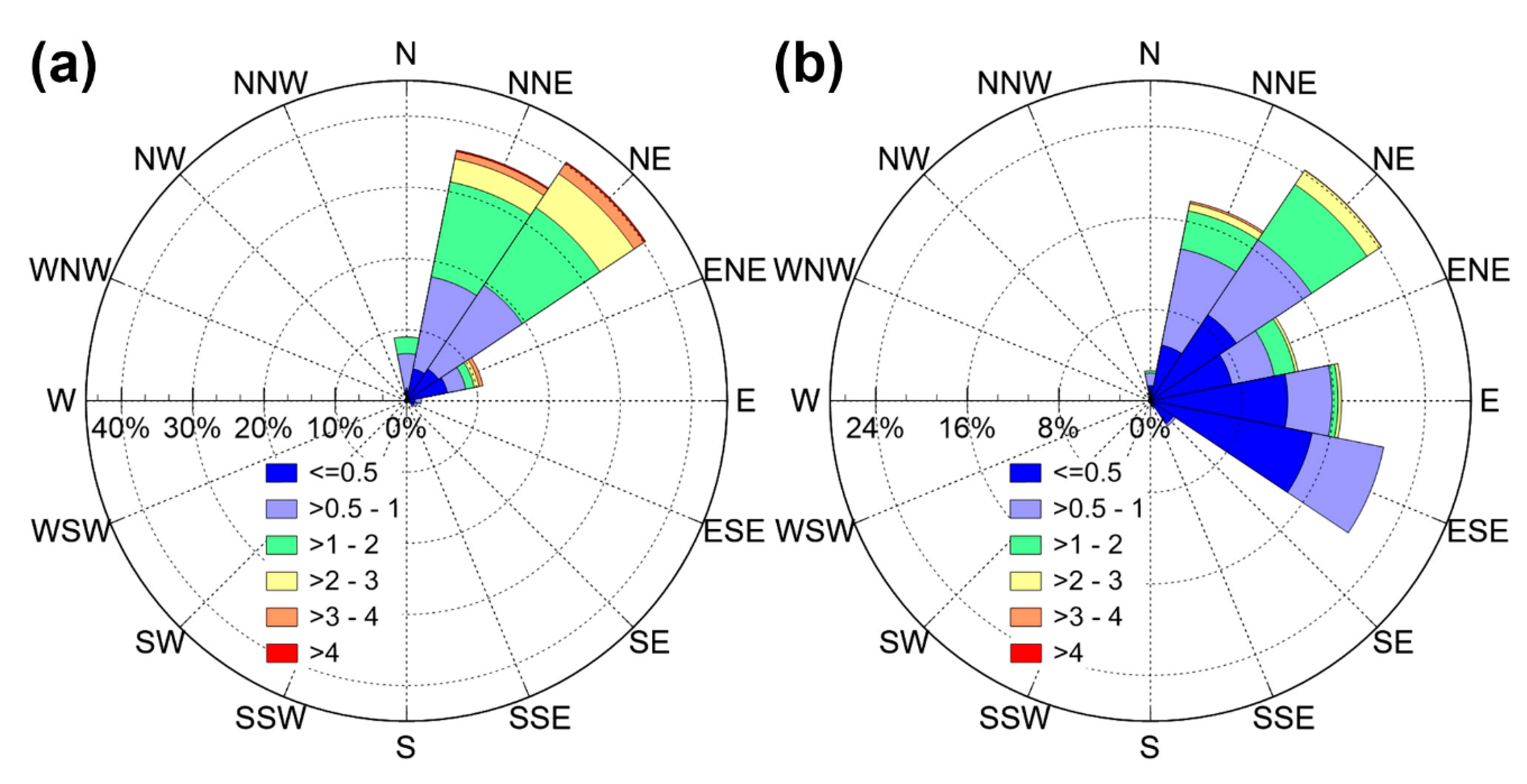
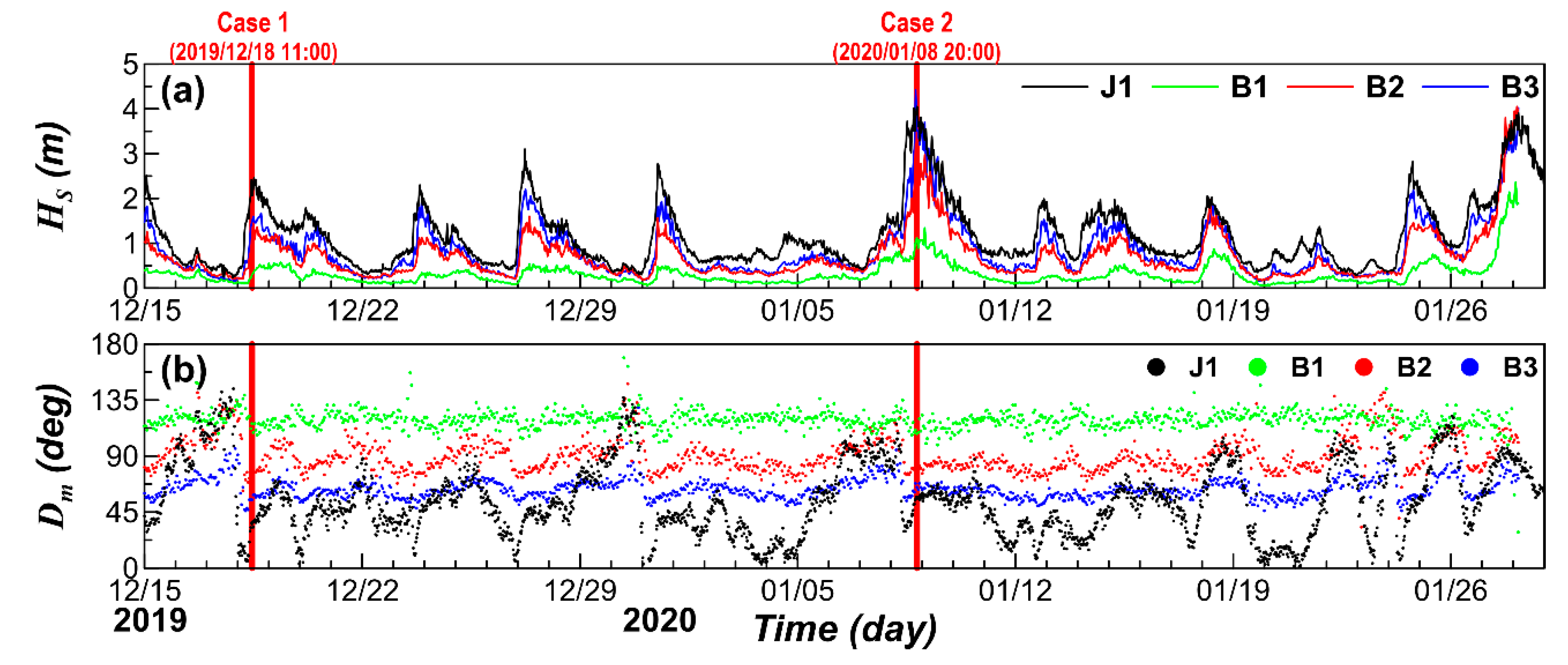
3.1. Wave Observation

In Figure 5, the time variations of the wave data measured during the field experiment were compared among the wave stations. In this period, seven storm waves were affiliated with the study site by defining the event of storm waves when the maximum $H_s$ exceeded 2 m. The first event occurred on 18 December 2019, when the maximum $H_s$ reached 2.36 m at wave station J1. The biggest storm event occurred on 8 January 2020, when the maximum $H_s$ at J1 reached 3.81 m. As listed in Table 1, these two events were selected and set-up for the model runs as Case 1 and Case 2, respectively. Figure 5a shows that the wave height significantly decreased as the waves propagated from J1 to B1. In Case 1, for example, $H_s$ was 2.36 m at J1, which was reduced to 1.48 m at B3, 1.05 m at B2, and 0.3 m at B1. Therefore, $H_s$ at B1 was only ~12.7% of that measured at J1. In Case 2, $H_s$ was 3.81 m at J1, but reduced to 3.53, 2.74, and 1.12 at B3, B2, and B1, respectively, resulting in a 29.4% reduction in wave height at B1 compared to that at J1. The reason for the reduction in the wave height was due to the wave transformation, specifically by the diffraction, which was indicated by the pattern of the wave direction changes, as shown in Figure 5b. In the figure, $D_m$ significantly changes along the path of the wave propagation. For J1, $D_m$ shows severe fluctuations because the waves propagated in various directions, outside the port. As the waves approached closer to the port, however, the fluctuations became smoother and the averaged value of $D_m$ increased, indicating that the wave propagating direction changed toward the port’s entrance. For example, for B3, $D_m$ fluctuated around 60$°$ (ENE) and around 90$°$ (E) for B2. In the onshore station, B1, however, $D_m$ was stable around 120$°$ (ESE). This rapid change in the wave direction in the lee area of the BW confirms the effect of the wave diffraction and also indicates that the significant reduction in $H_s$ along with the wave propagation (Figure 5a) could be closely related to the diffraction as well.

3.2. Model Comparison

In this section, the results from the two numerical models were compared based on the observational data for the two cases listed in Table 1. From the field experiment, the wave parameters, $H_s$ and $D_m$, were measured at each wave station (i.e., B1, B2, and B3) for Case 1 and Case 2 statistically using the spectra. TOMAWAC directly calculated these two parameters from the modeled spectra. In the case of ARTEMIS, the modeled data were analyzed to estimate these wave parameters. In order to estimate the wave propagating directions from ARTEMIS, it was necessary to run the phase-resolving model in the regular wave mode, forcing the model with a single wave height and period. Figure 6 shows an example of a wave propagation pattern that resulted from ARTEMIS using the regular wave mode in Case 2. It shows the distribution of the sea surface elevation at a given time step, indicating that the lines of the wave crests were clearly developed along the propagation. The figure also shows that the waves were transformed by changing directions as they approached the port. The wave height and direction could be calculated at each wave station by measuring the crest height and its propagating direction. However, model results in the regular wave mode would be less accurate, because the forcing conditions with only one wave height, period, and direction might lead to errors when applied along the whole open boundaries. Alternatively, ARTEMIS in Case 2 used the irregular wave mode in which the wave spectra from the phase-averaged model were also used as the boundary condition for this phase-resolving model. In this mode, the model results would not show the pattern of the wave propagation like the regular wave mode. Instead, the wave heights could be calculated from the distribution of the sea surface elevation field of the irregular waves. The wave propagation direction could not be evaluated in the irregular wave fields. Therefore, model validation and comparison with other phase-averaged models were only available for the wave height and not for the wave direction.

In Figure 7, the distributions of the wave heights were contoured for a comparison of the results from TOMAWAC and ARTEMIS, in Case 1. The result by ARTEMIS was from the irregular mode run, and that from the regular mode was not included in the comparison. The pattern of wave height distribution was similar between the two wave models in the TELEMAC system, as the effect of the wave transformation in the model was clearly reflected in both TOMAWAC and ARTEMIS. In both models, the wave height was reduced along the path of the wave propagation, as it was sufficiently small to secure the harbor’s tranquility ($\ll 1 \mathrm{m}$) inside the port. The differences between the models’ results were quantified through a comparison of the wave heights calculated at the wave stations, as listed in

Table 2. List of the wave parameters calculated from the model results, Case 1. The percentages in the parenthesis are the model errors from the observations.

Case 1	B1		B2		B3
	${\mathit{H}}_{\mathit{s}}$	${\mathit{D}}_{\mathit{m}}$	${\mathit{H}}_{\mathit{s}}$	${\mathit{D}}_{\mathit{m}}$	${\mathit{H}}_{\mathit{s}}$	${\mathit{D}}_{\mathit{m}}$
Observation	0.30 m	116.0°	1.05 m	78.0°	1.48 m	55.0°
TOMAWAC	0.22 m (27%)	107.3° (8%)	1.06 m (1%)	72.4° (7%)	1.53 m (3%)	57.1° (4%)
ARTEMIS (irregular)	0.28 m (7%)	-	1.09 m (4%)	-	1.58 m (7%)	-

. At B3, the outermost station from the port, $H_s$ was 1.48 m according to field observations. The model results were similar, 1.53 m (TOMAWAC), and 1.58 m (ARTEMIS), indicating that the error by ARTEMIS was larger. This difference was also observed at B2, as the error in modeling the wave height was smaller in TOMAWAC (1.06 m) than in ARTEMIS (1.09 m) compared to the observation (1.05 m). At B1, the innermost station, however, the error was smaller in ARTEMIS (0.28 m) than that in TOMAWAC (0.22 m), compared to the observation (0.30 m). The results of the wave height, as listed in Table 2, can be summarized as follows. For Case 1, the wave height was overestimated by both of the models at the two outer wave stations (B2 and B3) but underestimated at the innermost station (B1). In addition, the accuracy of the modeling was similar between the phase-averaged and phase-resolving models, with slightly more accurate data for TOMAWAC at the two outer stations. However, the wave height was more accurately modeled by ARTEMIS at the innermost station, indicating that the wave transformation effect was better simulated by the model as the waves approached the port behind the BW. These results are only for Case 1 in which the wave energy was moderate, but the waves propagated in a more acute angle outside the port (i.e., the angle between the BW and the wave propagation direction at J1 was larger).

In Figure 8, the distribution of the wave propagation direction, $D_m$, is contoured from the results of TOMAWAC, in Case 1. It is of note that the wave direction could not be estimated from the irregular mode of ARTEMIS, and its wave direction data are not included in the figure. It shows that the waves were gradually changing direction as they approached the shore. In particular, the directional change became more drastic near the shadow zone in the lee area of the BW, confirming the wave transformation by diffraction and/or refraction. It is of note, however, that the $D_m$ distribution became complicated near the coastal structures of the headland (HB) and submerged breakwaters (SBs). In Table 2, the $D_m$ calculated by the TOMAWAC are compared with observations as well. It shows that the modeled data agreed reasonably well with the observation, within an error range less than 10% (B1 = ~8%; B2 = ~7%; B3 = ~4%), confirming that the $D_m$ increased (i.e., the wave direction changed from NE to SE while approaching the port). It also shows that the errors increased as the waves approached closer to the port, which is discussed in Section 4.

The wave heights and directions were also similarly compared in Case 2. It is noted that the wave condition in Case 2 was more energetic than that in Case 2. As shown in Table 1, the wave height applied for the model boundary condition was 3.81 m in Case 2, whereas it was 2.36 m in Case 1. In this region, the waves with heights greater than 2 m were categorized as storm waves [22]; thus, both Case 1 and 2 corresponded to storm conditions. In particular, an $H_s$ of 3.81 m in Case 2 was an extreme wave condition, which was observed less than 5% during the whole year, as shown in Figure 2. The wave propagating directions were also different between the two cases. In Case 1, the $D_m$ was 36.40$°$, indicating that the waves outside the port approached in the NNE direction. In Case 2, the $D_m$ was 57.33$°$, showing that the waves approached in the NE/ENE direction. Therefore, the difference in the angles of the propagating waves when they reached the BW could influence the effectiveness of the models in simulating the wave transformation between the two cases.

In Figure 9, the wave height distributions are compared between the TOMAWAC and ARTEMIS, in Case 2. Compared to that in Case 1 in Figure 7, the distribution pattern showed larger discrepancies between the results of the two cases. For example, the wave height varied more smoothly in space, by TOMAWAC, as the waves propagated. In the case of ARTEMIS, the wave height varied more roughly in space, indicating that the wave transformation occurred unevenly along the propagation. In addition, the wave height was reduced more rapidly by ARTEMIS, as can be seen by comparing the wave height isolines of 3 and 1 m between the two models, indicating that the waves were more effectively transformed by ARTEMIS. These observations are confirmed from the comparison of the wave heights calculated at the wave stations, as listed in

Table 3. List of wave parameters calculated from the model results, Case 2. The percentages in the parenthesis are the model errors from the observations.

Case 2	B1		B2		B3
	${\mathit{H}}_{\mathit{s}}$	${\mathit{D}}_{\mathit{m}}$	${\mathit{H}}_{\mathit{s}}$	${\mathit{D}}_{\mathit{m}}$	${\mathit{H}}_{\mathit{s}}$	${\mathit{D}}_{\mathit{m}}$
Observation	1.12 m	108.0°	2.74 m	78.0°	3.53 m	65.0°
TOMAWAC	1.99 m (78%)	111.1° (3%)	3.09 m (13%)	93.8° (19%)	3.10 m (12%)	77.0° (18%)
ARTEMIS (Irregular)	1.16 m (4%)	-	2.79 m (2%)	-	3.09 m (13%)	-

. First, it is of note that the wave heights were underestimated at B3, the outermost wave station, by both models, where the $H_s$ was observed as 3.53 m. The wave heights calculated by the models were 3.10 m in TOMAWAC and 3.09 m in ARTEMIS, at B3, with an error of ~12%. When the waves reached station B2, however, the modeled data were overestimated, as $H_s$ was 2.74, 3.09, and 2.79 m from the observation, TOMAWAC, and ARTEMIS, respectively, with errors of ~13% (TOMAWAC) and ~2% (ARTEMIS), showing that the accuracy was significantly enhanced by ARTEMIS at B2. At the innermost station, B1, the wave height continued to be overestimated, as $H_s$ was 1.12, 1.99, and 1.16 m by the observation, TOMAWAC and ARTEMIS, respectively, with errors of ~78% (TOMAWAC) and ~4% (ARTEMIS), showing a large discrepancy in the accuracy between the two models.

In Figure 10, the distribution of the wave propagation direction, $D_m$, calculated by TOMAWAC, is contoured in Case 2. It shows that the waves that propagated with a $D_m$ of ~60$°$ changed directions according to the wave transformation as they approached the shore. However, the pattern of the $D_m$ isolines became more complicated near the coastal structures of the HB and SB and also near the port, which corresponded to the $H_s$ distribution in Figure 9a. This complexity can also be confirmed quantitatively through a comparison of the $D_m$ values, as listed in Table 3. At B3, the observed value of the $D_m$ was 65.0$°$, whereas it was 77.0$°$ by TOMAWAC, showing an error of ~18%. At B2, the error was ~19%, similar to that at B3 with a $D_m$ of 78.0$°$ and 93.8$°$ by observation and TOMAWAC, respectively. At B1, however, the error was significantly reduced to ~3%, which is in contrast to the wave height distribution, as the error of $H_s$ was greatest at B1 by TOMAWAC. The complex pattern of the wave heights and directions by the models is discussed in the next section.

The results in Table 1 and Table 2 indicate that there was a difference in the modeling performance between the two cases. In Case 1, the wave energy was lower than that in Case 2, but the wave incident angle to the BW was more acute in approaching the port entrance (i.e., the angle between the BW and the wave propagation direction at J1 was smaller). In both cases, the degree of the errors by ARTEMIS was comparable at all wave stations, ranging 2–13%. However, the error by TOMAWAC increased as the waves propagated toward the port entrance, and the error range became much larger in Case 2 in which the TOMAWAC error was 12% at B3 but increased to 78% at B1. In Case 1, the TOMAWAC error was 3% at B3 and 27% at B1. A discrepancy between the two cases was also observed in terms of the pattern of the errors. For example, the largest error by TOMAWAC was observed in Case 2 at B1, which was an overestimation (observation = 1.12 m; TOMAWAC = 1.99 m). In contrast, the error in Case 1 at B1 was caused by an underestimation (observation = 0.30 m; TOMAWAC = 0.22 m). These results indicate that the wave height calculated by TOMAWAC was reduced too much in Case 1 but not sufficiently reduced in Case 2, whereas the wave energy attenuation was reasonably simulated by ARTEMIS, which is discussed in the next section.

4. Discussion

One of the important results that should be noted from the numerical experiment is the inconsistency of the models’ accuracy. It was expected that the TELEMAC–ARTEMIS phase-resolving wave propagation model that solves the mild-slope equation would be more accurate than the TELEMAC–TOMAWAC phase-averaged model based on the wave action balance equation. In fact, the modeling error was lower for TOMAWAC at B2 and B3 in Case 1 and at B3 in Case 2. At the innermost location, B1, the error by ARTEMIS was lower for both cases, confirming that the model’s accuracy of ARTEMIS increased as the waves propagated to the port’s entrance behind the BW. In the outermost location, B3, however, the accuracy of ARTEMIS was lower than that of TOMAWAC in both cases.

The reason for the low model accuracy of TELEMAC–ARTEMIS outside the shadow zone is not yet clearly understood. However, one possible scenario can be found from the interference of the waves that were reflected from the complicated coasts around the HB and SB, in the lee area of location B3 (Figure 1b). In Figure 11, the wave height distributions in Figure 9 are compared between the two models at a magnified view that focuses on the area around the coastal structures in the lee area of B3, in Case 2. It clearly shows that the spatial variation of the $H_s$ distribution was smoother in the case of the TOMAWAC results. In contrast, the distribution by ARTEMIS was rough, as spots of lower and higher $H_s$ magnitudes developed in this area. The irregular pattern of the $H_s$ distribution by ARTEMIS was likely due to the fact of wave interference. In TOMAWAC, the effect of wave reflection was not considered, whereas the reflection effect was considered in ARTEMIS by setting the reflection coefficient along the coastline. Therefore, in the case where the coastline became complicated due to the construction of various coastal structures, such as the HB and SB in this study, it was difficult to precisely determine the reflection coefficients of the different structures and of the sandy shorelines. The purpose of the present study was to compare the model performance between the TOMAWAC and ARTEMIS, while the reflection coefficient was not set-up for the TOMAWAC boundaries. For fairness with respect to the model conditions, only the default values were given for the ARTEMIS boundaries, and they were not specified for different structures. Therefore, it is not meaningful to decide which model provided the better performance in this area. However, the results indicate that it is important to precisely determine the reflection coefficients along complicated coastlines, specifically near coastal structures that have different reflectance, and a model’s accuracy could decrease if this parameter is not carefully considered. In terms of the wave transformation by refraction/diffraction, it turned out that ARTEMIS showed better performance, as expected from phase-resolving models. For example, the results were more accurate by ARTEMIS at the innermost wave station, B1, in both Case 1 and 2. In TOMAWAC, the modeled wave heights were either underestimated (Case 1) or overestimated (Case 2), indicating that the phase-average model had no specific error pattern in calculating the wave transformation effect.

Regardless of the errors observed in the results from ARTEMIS, it is clear that this phase-resolving model provided better performance in modeling the effect of wave transformation in the port’s shadow zone, which was confirmed by the reasonable agreement with the observations at the innermost location, B1, in both cases. As expected, the accuracy of the TOMAWAC was lower in both cases. However, the pattern of errors showed a difference between the two cases, as the phase-averaged model was underestimated (i.e., the wave height was reduced more than the observed value) at the innermost location in Case 1 but severely overestimated in Case 2. The difference between the two cases in the performance of the TOMAWAC in calculating the wave transformation effect was also observed in the rate of wave height reduction estimated between B1 and B3, the innermost and outermost locations in the port’s shadow zone. In Case 1, the wave height at B1 was only ~14% (0.22 m/1.53 m), whereas it was ~64% (3.10 m/1.99 m) in Case 2.

The fact that the wave height reduction rate was greater in Case 1 could not be understood by simply considering Equations (2) and (3), which describe the wavelength change caused by wave diffraction in the TOMAWAC. By assuming that the $\nabla \mathrm{a}$ was similar between the two cases, $\mathsf{\delta }$ ($\propto 1/\mathrm{a}$) would be greater in Case 2 in which the $H_s$ was greater. Therefore, the change in the wave number by diffraction would be greater in Case 2, according to the implication of Equation (2). However, the deformation of the propagating waves was greater in Case 1 not only in the wave height but also in the wave direction. Although the reason for this discrepancy is not yet clearly understood, it is likely that the lower modeling performance by TOMAWAC in Case 2 was due to the difference in the wave incident angles. In Case 1, the waves approached the shadow zone at a more acute angle outside the port, compared to the waves in Case 2. Therefore, it was easier for the waves to reach the inner area of the shadow zone in Case 2, even though the effect of the wave diffraction was not effectively calculated by this phase-averaged model. In Case 1, the waves should be diffracted more by the model to reach the inner part of the shadow zone (i.e., changing the wave propagating direction more sharply in the shadow zone). Because the model’s performance for wave transformation was less effective for TOMAWAC, however, the waves could not sufficiently reach the innermost location, reducing the wave height at B1 excessively in Case 1. For ARTEMIS, the wave diffraction was effectively simulated so that the wave energy was successfully transferred to the innermost location regardless of the wave incident angles. The results of this study provide important implications for engineering aspects. Although phase-averaged models such as the TELEMAC–TOMAWAC have been largely applied in engineering practices due to the economic computational cost, the results of this study suggest that phase-resolving wave models are recommended in estimating the morphological and shoreline changes caused by wave transformation around coastal structures.

5. Conclusions

The numerical and field experiments in the present study were conducted to compare the performance of modeling the wave transformation effect using real field data measured near the shadow zone in the lee area of a breakwater which had been constructed to secure the harbor’s tranquility. The two models were selected from wave propagating models installed in the TELEMAC system. TOMAWAC is a phase-averaged model based on the wave action balance equation, and ARTEMIS is a phase-resolving model that solves the mild-slope equation. They were set-up in the same computational domain with unstructured grids to facilitate the comparison. Two cases of wave conditions were constructed based on the wave observations outside the port, and the model performances were tested through comparisons of the wave data measured at three locations in the lee area of the port breakwater.

It was expected that the phase-resolving model would be better at modeling the wave transformation, which was confirmed as the ARTEMIS data showed higher accuracy at the innermost location in both test cases of different wave heights and propagating wave directions. Outside the shadow zone, however, ARTEMIS showed no better performance than TOMAWAC in terms of the error in modeling the wave height. The findings and their implications from this study are listed as follows:

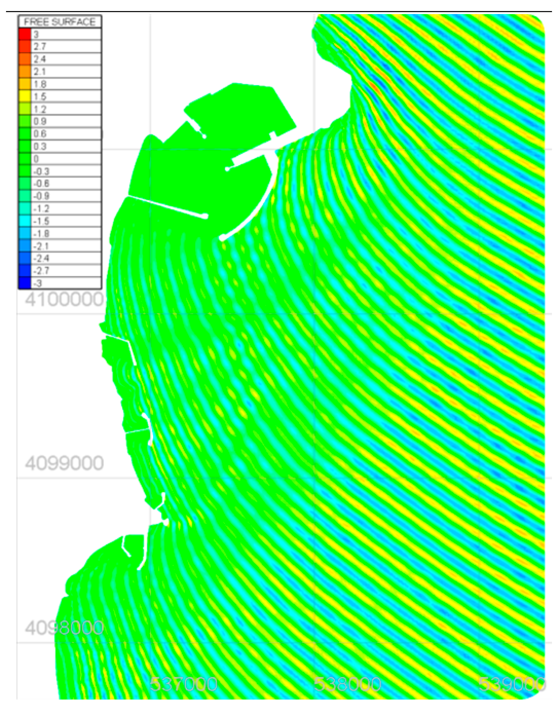
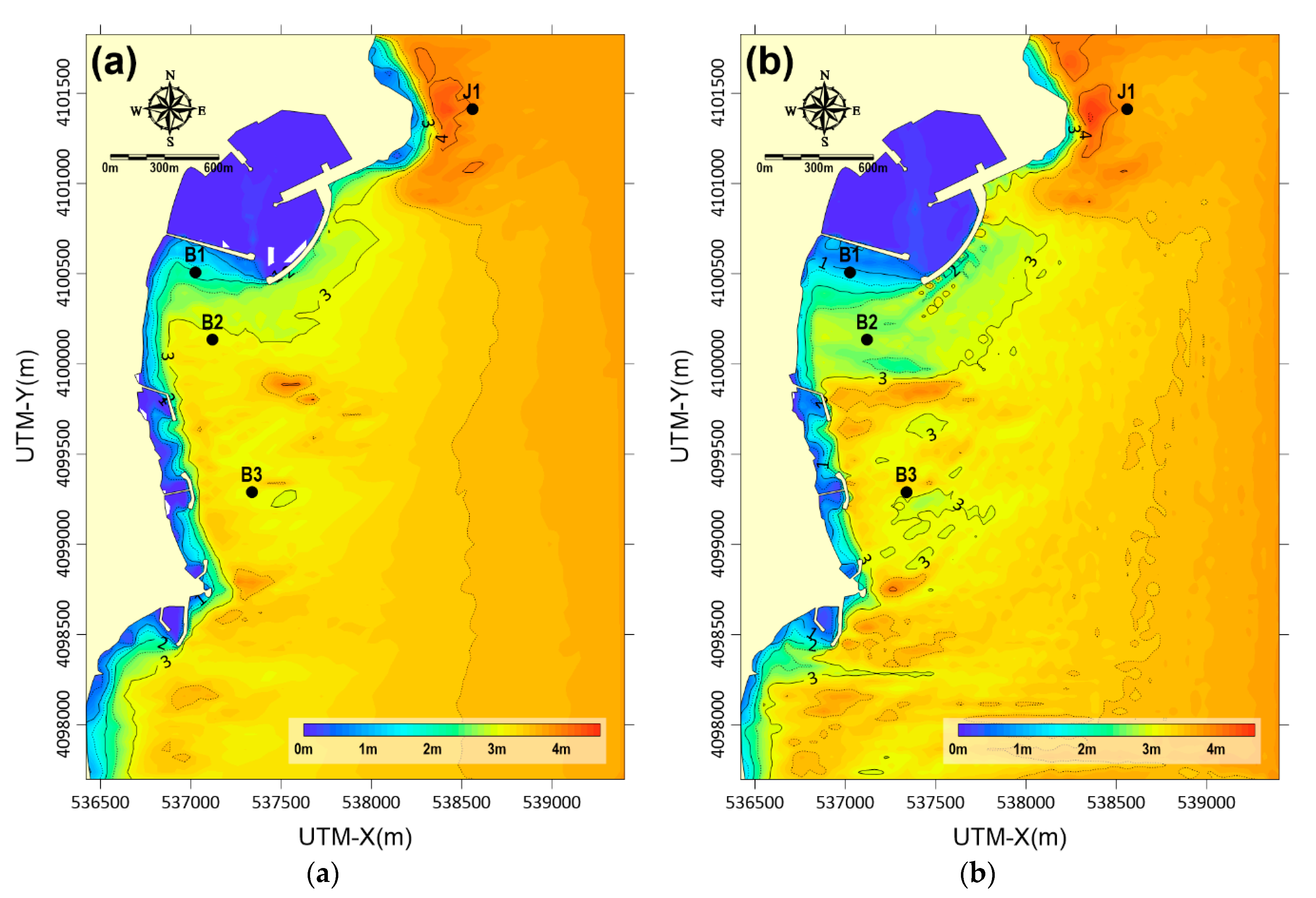
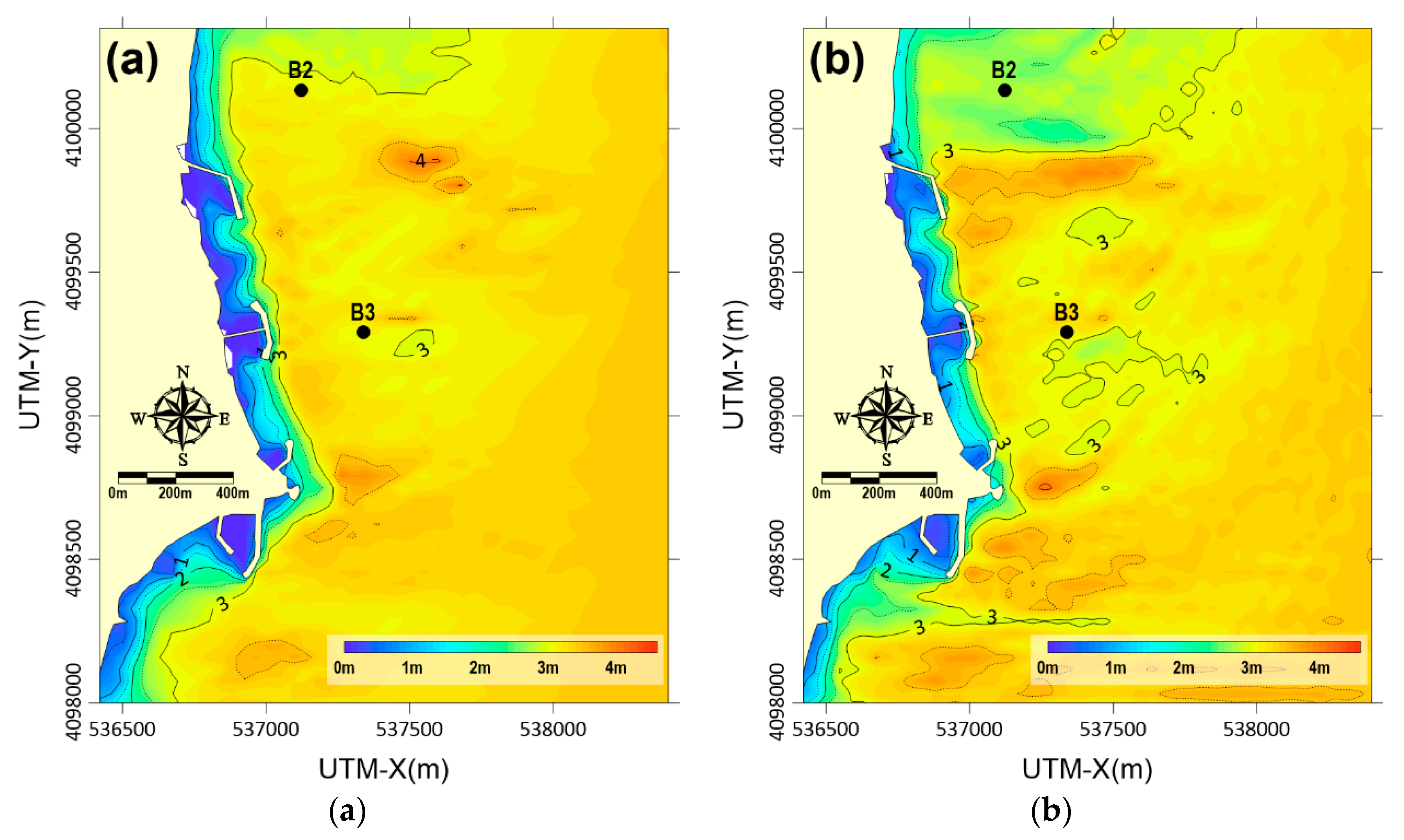
• The wave heights calculated by ARTEMIS decreased as the waves approached the ports, showing good agreement with the observed wave height data in both cases. The errors estimated were less than 10%, except for one wave station located at the outermost part of the shadow zone, indicating that the wave transformation effect (i.e., refraction/diffraction) was nicely modeled by this phase-resolving model.
• The performance of TOMAWAC showed less accuracy in terms of the wave height that was underestimated (lower wave height than observation) or overestimated in the innermost location.
• Although the pattern of errors in the TOMAWAC’s wave heights was opposite (underestimation vs. overestimation), both might be due to the poor performance in modeling the wave transformation by this phase-averaged model. It was likely that the underestimation was because the wave energy could not be successfully transferred to the innermost location due to the acute angle behind the breakwater that disturbed the wave energy propagation with diffraction. The overestimation in the second case might have occurred because the wave energy could reach the innermost location disproportionally even though the diffraction effect was not successfully implemented due to the less acute angle of the incident waves.
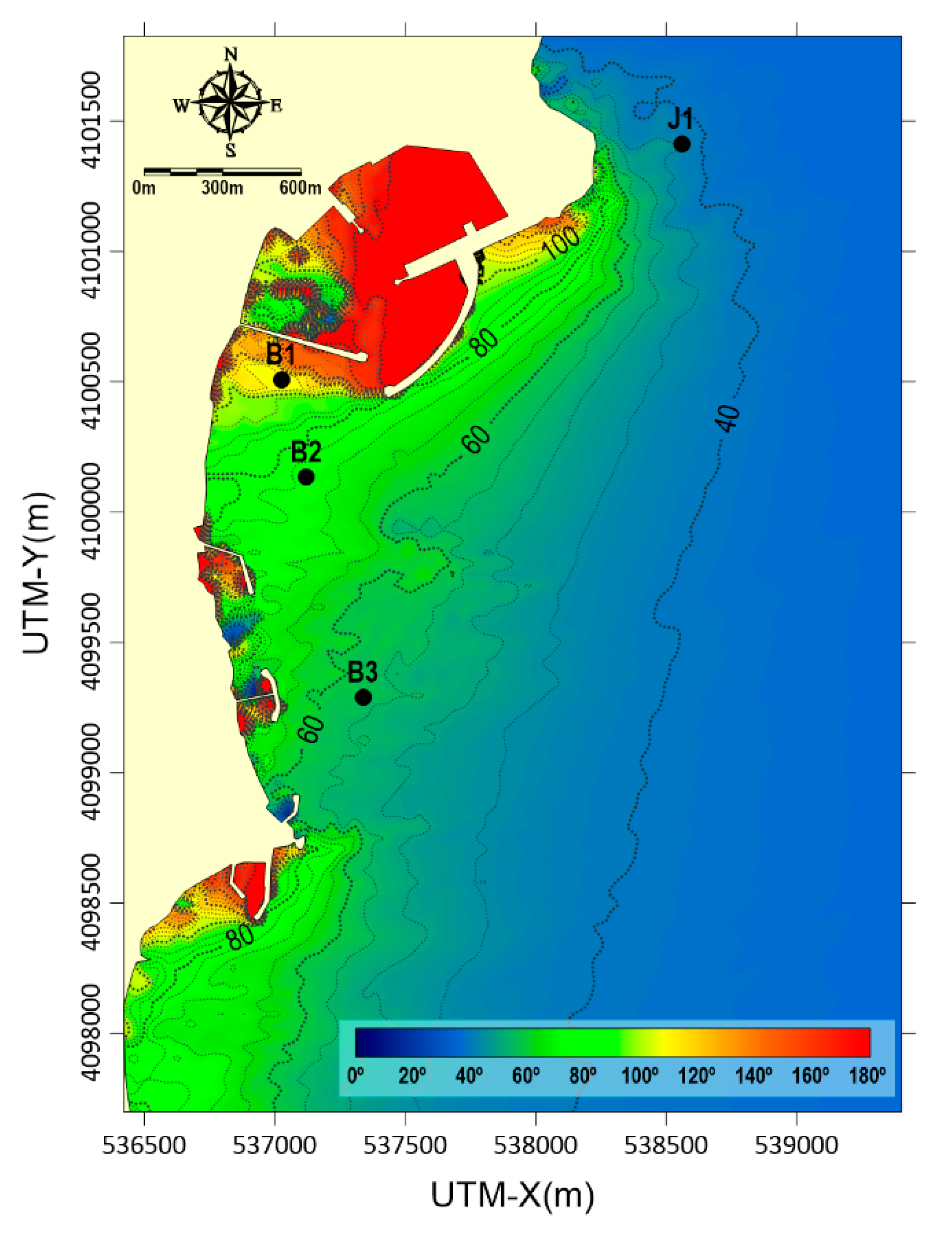
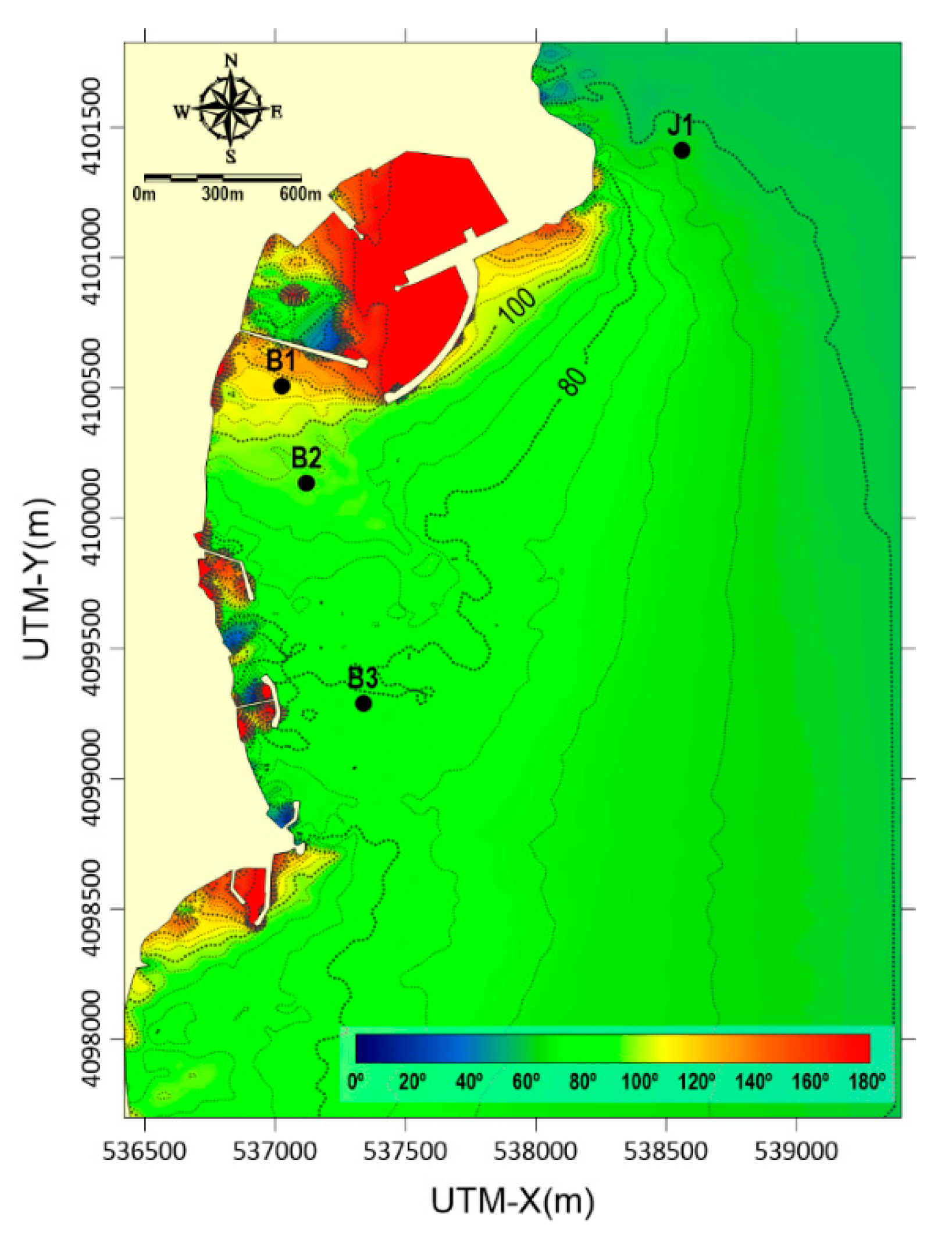
• Wave directions modeled by the TOMAWAC support the above results. In the first case (wave height underestimation), the observed wave direction was 116° at the innermost location, whereas it was ~107° by the model, which indicates that the wave propagation direction was not sufficiently changed by the TOMAWAC, and the diffraction effect was not successfully modeled. In the second case (overestimation), the modeled wave direction changed by only 34°, as the waves propagated from the outermost to the innermost location, whereas the observational data changed by 43°, indicating that the modeled wave height was not reduced as much as the observation, because the effect of the wave diffraction could not be successfully applied during the propagation process and the wave energy was transferred to the innermost location without significant loss by the transformation.
• Although the ARTEMIS results were in better agreement with the measured wave heights in the inner locations in both cases, confirming its successful performance in modeling the wave transformation, it provided higher errors in the outermost location than TOMAWAC. The reason was likely because the coastlines near this outermost location become complicated due to the construction of coastal structures, which required high accuracy in setting the reflection coefficient along the complex land boundaries. Otherwise, the model would result in a wave in which the propagating waves were mixed with the falsely reflected waves, which could increase the errors compared to a real wave field.

The results of this study only compared the performance of two wave models in simulating the wave diffraction effect around a breakwater based on field measurements. However, the outcomes of this study could be further applied in planning protection measures for coastal sandy shorelines and habitats. For example, both model results indicate that the wave energy could be significantly reduced in the lee area of the breakwater, which could cause the alongshore movement of sediments if they happened to be sandy beaches. In protecting the beach from erosion, the breakwater (or other coastal interventions) should be carefully designed. In many engineering practices, phase-averaged models such as the TELEMAC–TOMAWAC have been largely applied. The results of the present study, however, suggest that phase-resolving wave models are recommended to be coupled with the sediment transport models in estimating the morphological and shoreline changes caused by the wave transformation around such structures. Even then in that case, these phase-resolving models should be carefully tuned, specifically in the areas of complex coastlines because the model accuracy would decrease unless the wave reflection effects at the shore were to be accurately considered.

References

1. Zhang, K.; Douglas, B.C.; Leatherman, S.P. Global warming and coastal erosion. Clim. Chang. 2004, 64, 41–58. [Google Scholar] [CrossRef]
2. Mentaschi, L.; Vousdoukas, M.I.; Pekel, J.F.; Voukouvalas, E.; Feyen, L. Global long-term observations of coastal erosion and accretion. Sci. Rep. 2018, 8, 12876. [Google Scholar] [CrossRef] [Green Version]
3. Do, J.D.; Jin, J.-Y.; Jeong, W.M.; Lee, B.; Choi, J.Y.; Chang, Y.S. Collapse of a coastal revetment due to the combined effect of anthropogenic and natural disturbances. Sustainability 2021, 13, 3712. [Google Scholar] [CrossRef]
4. Do, J.D.; Jin, J.-Y.; Hyun, S.K.; Jeong, W.M.; Chang, Y.S. Numerical investigation of the effect of wave diffraction on beach erosion/accretion at the Gangneung Harbor, Korea. J. Hydro-Environ. Res. 2020, 29, 31–44. [Google Scholar] [CrossRef]
5. Maa, J.P.-Y.; Hsu, T.-W.; Tsai, C.-H.; Juang, W. Comparison of wave refraction and diffraction models. J. Coast. Res. 2000, 16, 1073–1082. [Google Scholar]
6. Dezvareh, R.; Bargi, K.; Moradi, Y. Assessment of Wave Diffraction behind the Breakwater Using Mild Slope and Boussinesq Theories. Int. J. Comput. Appl. Eng. Sci. 2012, 2, 72–76. [Google Scholar]
7. Han, X.; Dong, S.; Wang, Y. Interaction between oblique waves and arc-shaped breakwater: Wave action on the breakwater and wave transformation behind it. Ocean Eng. 2021, 234, 109252. [Google Scholar] [CrossRef]
8. Afentoulis, V.; Papadimitriou, A.; Belibassakis, K.; Tsoukala, V. A coupled model for sediment transport dynamics and prediction of seabed morphology with application to 1DH/2DH coastal engineering problems. Oceanologia 2022, 64, 514–534. [Google Scholar] [CrossRef]
9. Sorensen, R.M. Wave refraction, diffraction, and reflection. In Basic Coastal Engineering; Springer: Boston, MA, USA, 2006; pp. 79–111. [Google Scholar]
10. Panigrahi, J.K.; Padhy, C.; Murty, A. Inner harbour wave agitation using boussinesq wave model. Int. J. Nav. Archit. Ocean. Eng. 2015, 7, 70–86. [Google Scholar] [CrossRef] [Green Version]
11. Lesser, G.R.; Roelvink, J.V.; van Kester, J.T.M.; Stelling, G. Development and validation of a three-dimensional morphological model. Coast. Eng. 2004, 51, 883–915. [Google Scholar] [CrossRef]
12. Hervouet, J.-M. Hydrodynamics of Free Surface Flows: Modelling with the Finite Element Method; John Wiley & Sons: Hoboken, NJ, USA, 2007. [Google Scholar]
13. Nam, P.T.; Larson, M.; Hanson, H. A numerical model of beach morphological evolution due to waves and currents in the vicinity of coastal structures. Coast. Eng. 2011, 58, 863–876. [Google Scholar] [CrossRef]
14. Tang, J.; Lyu, Y.; Shen, Y.; Zhang, M.; Su, M. Numerical study on influences of breakwater layout on coastal waves, wave-induced currents, sediment transport and beach morphological evolution. Ocean. Eng. 2017, 141, 375–387. [Google Scholar] [CrossRef]
15. Afentoulis, V.; Eleftheria, K.; Eleni, S.; Evangelos, M.; Archontia, L.; Christos, M.; Vasiliki, T. Coastal Processes Assessment under Extreme Storm Events Using Numerical Modelling Approaches. Environ. Process. 2017, 4, 731–747. [Google Scholar] [CrossRef]
16. Ding, Y.; Wang, S.S. Development and application of a coastal and estuarine morphological process modeling system. J. Coast. Res. 2008, 10052, 127–140. [Google Scholar] [CrossRef]
17. Durand, N.; Bourban, S.; Tozer, N. ARTEMIS developments at HR Wallingford. In Proceedings of the XXV TELEMAC-MASCARET User Conference, Norwich, UK, 9–11 October 2018; pp. 131–135. [Google Scholar]
18. Nwogu, O.G. Numerical prediction of breaking waves and currents with a Boussinesq model. In Coastal Engineering 1996; American Society of Civil Engineers: Reston, VA, USA, 1997; pp. 4807–4820. [Google Scholar]
19. Kirby, J.T. Boussinesq models and their application to coastal processes across a wide range of scales. J. Waterw. Port Coast. Ocean. Eng. 2016, 142, 03116005. [Google Scholar] [CrossRef]
20. Karambas, T.V. Design of detached breakwaters for coastal protection: Development and application of an advanced numerical model. In Proceedings of the 33rd International Conference on Coastal Engineering, Santander, Spain, 1–6 July 2012; pp. 1–6. [Google Scholar]
21. Karambas, T.V.; Samaras, A.G. An integrated numerical model for the design of coastal protection structures. J. Mar. Sci. Eng. 2017, 5, 50. [Google Scholar] [CrossRef]
22. Klonaris, G.T.; Metallinos, A.S.; Memos, C.D.; Galani, K.A. Experimental and numerical investigation of bed morphology in the lee of porous submerged breakwaters. Coast. Eng. 2020, 155, 103591. [Google Scholar] [CrossRef]
23. Malej, M.; Shi, F.; Smith, J.M. Modeling Ship-Wake-Induced Sediment Transport and Morphological Change—Sediment Module in FUNWAVE-TVD; Coastal and Hydraulics Laboratory, Engineer Research and Development Center: Vicksburg, VI, USA, 2019. [Google Scholar]
24. Briere, C.; Abadie, S.; Bretel, P.; Lang, P. Assessment of TELEMAC system performances, a hydrodynamic case study of Anglet, France. Coast. Eng. 2007, 54, 345–356. [Google Scholar] [CrossRef]
25. Do, J.D.; Jin, J.-Y.; Jeong, W.M.; Lee, B.; Kim, C.H.; Chang, Y.S. Observation of nearshore crescentic sandbar formation during storm wave conditions using satellite images and video monitoring data. Mar. Geol. 2021, 442, 106661. [Google Scholar] [CrossRef]
26. Benoit, M.; Marcos, F.; Becq, F. Development of a third generation shallow-water wave model with unstructured spatial meshing. In Coastal Engineering 1996; American Society of Civil Engineers: Reston, VA, USA, 1997; pp. 465–478. [Google Scholar]
27. Booij, N.; Ris, R.C.; Holthuijsen, L.H. A third-generation wave model for coastal regions: 1. Model description and validation. J. Geophys. Res. Ocean 1999, 104, 7649–7666. [Google Scholar] [CrossRef] [Green Version]
28. Villaret, C.; Hervouet, J.-M.; Kopmann, R.; Merkel, U.; Davies, A.G. Morphodynamic modeling using the TELEMAC finite-element system. Comput. Geosci. 2013, 53, 105–113. [Google Scholar] [CrossRef]
29. Booij, N.; Holthuijsen, L.; Ris, R. The “SWAN” wave model for shallow water. In Coastal Engineering 1996; American Society of Civil Engineers: Reston, VA, USA, 1997; pp. 668–676. [Google Scholar]
30. Holthuijsen, L.; Herman, A.; Booij, N. Phase-decoupled refraction–diffraction for spectral wave models. Coast. Eng. 2003, 49, 291–305. [Google Scholar] [CrossRef]
31. Berkhoff, J.C.W. Mathematical Models for Simple Harmonic Linear Water Waves: Wave Diffraction and Refraction. Ph.D. Thesis, Delft University of Technology, Delft, The Netherlands, 1976. [Google Scholar]
32. De Jong, M.P.D.; Borsboom, M. A practical post-processing methods to obtain wave parameters from phase-resolving wave model results. Int. J. Ocean. Clim. Syst. 2012, 3, 203–216. [Google Scholar] [CrossRef]
Figure 1. (a) Map of the Korea Peninsula and the location of Jukbyeon Port (JP); (b) map of JP.
Jmse 10 02032 g001
Figure 2. Rose diagram: (a) winter (December 2019–February 2020); (b) summer (June–August 2020).
Jmse 10 02032 g002
Figure 3. (a) Aerial photo of the area near the HB and SB shown in Figure 1b, taken on 16 October 2005 and (b) 29 September 2010; (c) Google Earth image of the same site, taken on 3 March 2018.
Jmse 10 02032 g003
Figure 4. The unstructured grid system for TOMAWAC and ARTEMIS: (a) meshes around JP, with the smallest grid size of 5 m; (b) map of the water depths in the models based on bathymetry measurements.
Jmse 10 02032 g004
Figure 5. Time variations of the wave parameters during the field experiment: (a) significant wave height ( H s ) and (b) peak wave direction ( D m ) calculated from the wave spectra measured at the four wave stations shown in Figure 1b. Black: J1; green: B1; red: B2; blue: B3.
Jmse 10 02032 g005
Figure 6. Example of a pattern of sea surface elevation resulting from the regular wave mode of TELEMAC–ARTEMIS, Case 2.
Jmse 10 02032 g006
Figure 7. Distributions of wave heights modeled by (a) TELEMAC–TOMAWAC and (b) TELEMAC–ARTEMIS, Case 1.
Jmse 10 02032 g007
Figure 8. Distribution of the wave propagating direction, D m , modeled by TELEMAC–TOMAWAC, Case 1.
Jmse 10 02032 g008
Figure 9. Distributions of wave heights modeled by (a) TELEMAC–TOMAWAC and (b) TEL EMAC–ARTEMIS, Case 2.
Jmse 10 02032 g009
Figure 10. Distribution of the wave propagating direction, D m , modeled by TEL EMAC– TOMAWAC, Case 2.
Jmse 10 02032 g010
Figure 11. Same as Figure 9 but at a magnified view for comparison of the wave height distributions near the coastal structures, headland breakwaters, and submerged breakwaters, (a) TELEMAC–TOMAWAC and (b) TEL EMAC–ARTEMIS, Case 2.
Jmse 10 02032 g011