Article

Experimental Study on the Target–Receiver Formation Problem with the Exploitation of Coherent and Non-Coherent Bearing Information

1
Key Laboratory of Underwater Acoustic Signal Processing of Ministry of Education, Southeast University, Nanjing 210096, China
2
School of Marine Science and Technology, Northwestern Polytechnical University, Xi’an 710072, China
*
Author to whom correspondence should be addressed.
J. Mar. Sci. Eng. 2022, 10(12), 1922; https://doi.org/10.3390/jmse10121922
Submission received: 18 October 2022 / Revised: 20 November 2022 / Accepted: 23 November 2022 / Published: 6 December 2022
(This article belongs to the Special Issue Application of Sensing and Machine Learning to Underwater Acoustic)

Abstract

:
Localization of emitting sources is a fundamental task in sonar applications. One of the most important factors that affect the localization performance is the sensor–target geometry. The sensor formation problem is usually addressed in related work assuming that the target is static and the location is known to a certain degree, but this is not the case for many underwater surveillance problems. In this paper, we deal with the target–receiver formation problem from a different perspective, and propose to investigate the effect of target–receiver geometry on localization performance by exploiting the spatial spectrum of the direct position determination (DPD) methods. For a given multi-array system, the transformation of geometrical patterns can be explicitly demonstrated as the target moves along the track. Meaningful characteristics of the DPD methods are obtained from the experimental results, where coherent and non-coherent bearing information is used and compared. The feasibility of the DPD approaches in the ocean environments is also investigated by comparing with a matched filter processing (MFP)-based multi-array processor in order to validate the credibility of the results in this paper.

1. Introduction

The localization of emitting sources is a fundamental task in sonar and radar applications. Localization methods based on distributed multi-array systems can be categorized into two classes: the two-step methods and the direct localization methods. Classical two-step localization methods are based on intermediate measurements, such as angle of arrival (AOA) and time difference of arrival (TDOA). This issue has been extensively investigated for decades, leading to diverse research on bearings-only [1], TDOA-based [2], and hybrid [3] source localization methods. The direct localization methods, or specifically the direct position determination (DPD) methods, were firstly proposed by Weiss [4,5,6,7,8] and Bosse [9,10], which jointly process all the received signals, bypassing the parameter estimation step of the conventional two-step methods.
All of the estimators outlined above aim to improve the localization accuracy. It is well-known that one of the most important factors that affect the localization performance is the deployment of sensors or the design of trajectories for moving platforms. Given a specific localization problem, the optimal sensor formation in terms of localization accuracy is typically obtained by examining the corresponding Cramer–Rao bound (CRB) or the Fisher information matrix (FIM) [11]. The target location is commonly assumed to be static and known (exactly or with uncertainty) in the formulation of the optimization problems [12,13]. It seems unrealistic since in many underwater surveillance tasks, the target is not static and the location is to be estimated by the sonar systems. However, the solutions obtained can provide guidance for sensor placement at the first stage. Nevertheless, it is of importance to evaluate the target–receiver geometry regarding the localization accuracy for regular underwater sensing scenarios, which is rarely discussed in related work.
A useful characteristic of the DPD methods is that the contribution of each receiver is demonstrated in the 2D spectrum of the objective function. This characteristic is exploited in this paper to realize our objective, which is to investigate the localization performance of a fixed distributed receiving system with different target–receiver geometries as the target moves along its track. The optimal methodology of the direct localization concept is to consider the receiving arrays as sub-arrays of a large array, and a global sample covariance matrix (SCM) is obtained to estimate the source locations. In contrast, a non-coherent distributed array model is employed in [14,15,16,17], where the SCM of each receiving array is transmitted to the central station, and the correlation between disparate sensor arrays is considered irrelevant. From the perspective of information fusion, the above global coherent and non-coherent systems correspond respectively to the exploitation of coherent and non-coherent bearing information. Notably, it is shown in [18] that the power of the sub-array beams in the 2D spectrum is adjusted inherently (instead of through weights) within the global coherent SCM, which means that the bearing information of each sub-array may also be adjusted in the fusion process. In other words, the coherent bearing information of the sub-arrays is not triangulated as is the way with the non-coherent systems. Hence, it is of interest to investigate whether the target–receiver geometry has different effects on localization performance for the two different systems.
In order to evaluate the effect of target–receiver geometry on localization performance, as well as on the exploitation of coherent and non-coherent bearing information, two typical global coherent and non-coherent DPD methods are applied to the SWellEx-96 shallow water experiment data set [19], where three different source–receiver geometries are formed as the source moves along the track. The transformation of different geometrical patterns can be explicitly demonstrated in the whole procedure from the spatial ambiguous surface of the DPD methods. Experimental results lead to an interesting and useful geometrical interpretation of the relationship between sensor–target configuration and the localization performance of algorithms exploiting bearings-only information, which has not been reported in related work.
To guarantee the credibility of the results, the feasibility of the DPD methods in the ocean environments is to be assured. However, although the superiority of DPD methods over conventional two-step methods has been widely demonstrated for radar applications, little work has been reported on their application to multiple acoustic arrays for underwater target localization tasks. One consideration for the direct application of the DPD methods is the plane wave assumption. The assumption is adopted by many sonar array processing algorithms, such as various beamformers [20], but it may introduce a certain degree of error in some cases (e.g., when the aperture of the receiving array is too large or the target is near the endfire of the array) [21]. In contrast, matched-field processing (MFP) is a well-established technique in ocean acoustic source localization, which exploits acoustic waveguide propagation information in the estimation process. Recently, MFP-based multiple-array processors have been developed [22,23], and one of the MFP processors will be evaluated together with the two typical DPD methods to investigate the feasibility of the DPD methods.
The paper is organized as follows: Section 2 introduces two typical global coherent and non-coherent DPD methods. Section 3 evaluates the performance of the two DPD methods with different source–receiver geometries and tone frequencies, and presents a performance comparison between DPD and MFP processors. In Section 4, we summarize the advantages and limitations of these DPD methods in different scenarios.

2. Problem Description and Its Proposed Solution

Imagine that the multiple-array receiving system consists of L spatially distributed hydrophone arrays, each of them composed of N l 1 l L elements and receiving radiating narrowband signals from a known number of Q sources with a common center frequency f c . The total number of hydrophones is N = l N l . Using complex (analytic) signal representation, the observation vector of the lth array at time t can be expressed as
x l t = q = 1 Q ρ l , q a l p q s q t τ l p q + n l t ,
where ρ l , q is an unknown complex parameter representing the channel attenuation, and s q t 1 q Q are the unknown source signals. Assume that the sources and receivers are within the same plane, and the location of the qth source is expressed in Cartesian coordinates as p q = [ x , y , z ] T with z = 0 . a l p q is the steering vector of the lth array with respect to the qth source, whose ith element is e j 2 π f c ζ l , q , i and ζ l , q , i is the time delay between the ith sensor and the phase center of the lth array. τ l p q is the propagation time of the qth source signal to the lth array. We assume that the sources are located in the far-field of each array, which implies that the array response becomes a function of the AOA only, i.e., a l p = a l θ l p . The additive noise vector n l t is white Gaussian, uncorrelated with the signals, of zero mean and with covariance matrix σ l 2 I N l . σ l 2 is the unknown noise variance at the lth array. We assume that the impinging signals are narrowband across all arrays, which means the bandwidth is small compared to the inverse of the transmit time of a wavefront across the arrays. Under this assumption we can write s q t τ l p q s q t e j 2 π f c τ l p q .
Stacking the observations from all arrays at time t in a column vector yields
x = A s + n ,
where
x = [ x 1 T , , x L T ] T , s = [ s 1 , , s Q ] T , n = [ n 1 T , , n L T ] T , A = [ a ¯ 1 , , a ¯ Q ] , a ¯ q = [ ρ 1 , q a 1 T e j 2 π f c τ 1 p q , , ρ L , q a L T e j 2 π f c τ L p q ] T ,
and ( · ) T denotes the transpose operator.
In the following, we introduce two typical narrowband DPD approaches that will be applied to the SWellEx-96 horizontal array data set in Section 3. These approaches are based on two different array models: a global coherent large array model and a non-coherent distributed array model.

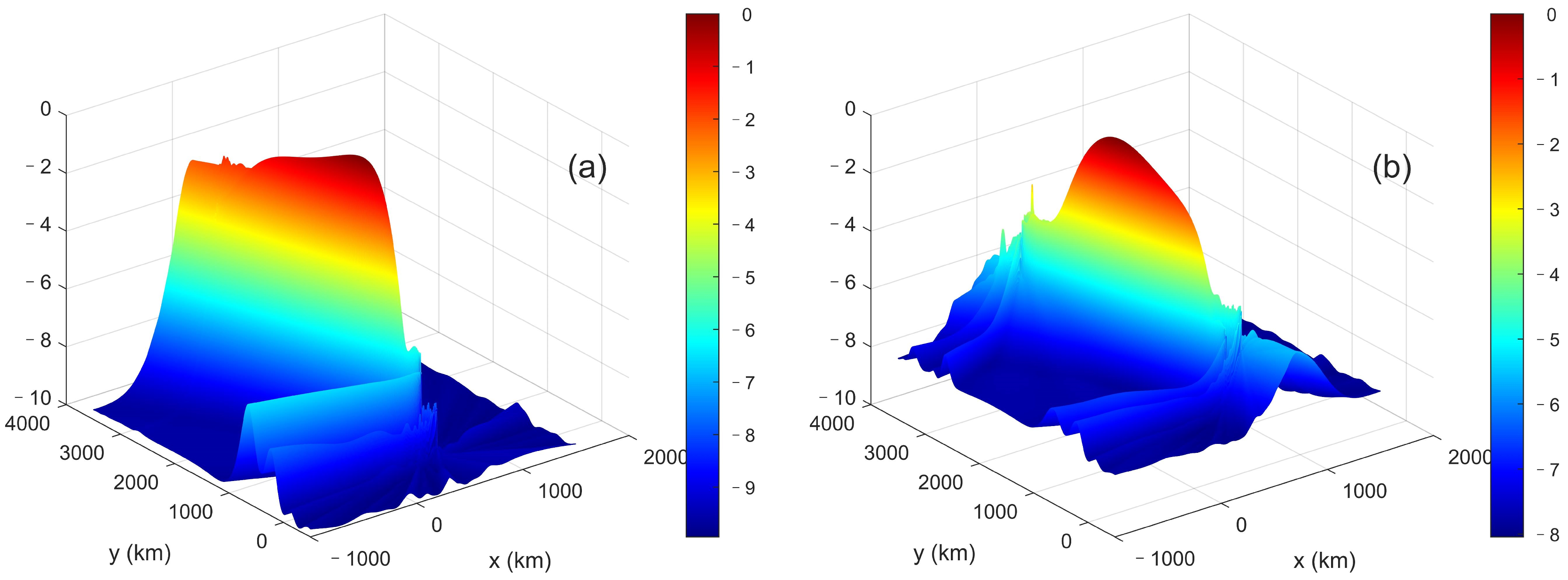
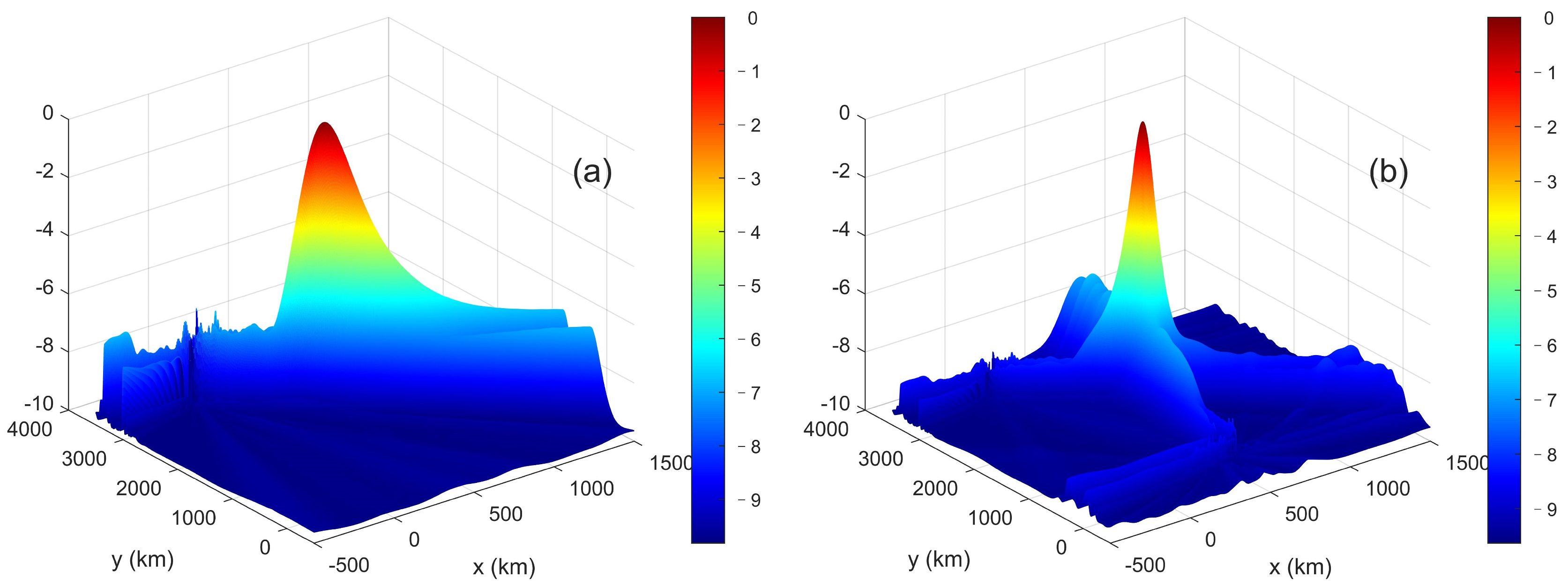
2.1. Global Coherent Processing

The global MUSIC algorithm (GMA) proposed by Bosse [9] is a global coherent position estimator. The covariance matrix (SCM) of the global large array is approximated by
R ^ = 1 T t = 1 T x t x H t ,
where T is the number of time samples. Following the MUSIC algorithm [24] and assuming the dimension of the signal subspace is Q, the unknown parameters are estimated by finding the Q zeros of the following objective function:
C ( p ) = a ¯ H ( p ) Π ^ n a ¯ ( p ) a ¯ H ( p ) a ¯ ( p ) ,
where a ¯ ( p ) is defined in Equation (3). Π ^ n = I U ^ s H U ^ s is the estimated noise projector, and the N × Q matrix Π ^ s is the estimated signal subspace, consisting of the Q eigenvectors of R ^ corresponding to its Q largest eigenvalues. Note that
a ¯ ( p q ) = U ( p q ) ρ ¯ q ,
where
ρ ¯ q = [ ρ 1 , q e j 2 π f c τ 1 p q , , ρ L , q e j 2 π f c τ L p q ] ,
U ( p ) = d i a g ( a 1 ( p ) , , a L ( p ) ) ,
and d i a g ( v ) is a diagonal matrix built with the entries in the vector v . Finding the minimum of the quadratic ratio Equation (5) is equivalent to searching the minimal eigenvalue of the matrix [ a ¯ H ( p ) a ¯ ( p ) ] 1 a ¯ H ( p ) Π ^ n a ¯ ( p ) [25]. For the sake of computational cost, the following equivalent criterion is preferred [26]:
C g ( p ) = | U H ( p ) Π ^ n U ( p ) | | U H ( p ) U ( p ) | ,
where | A | stands for the determinant of matrix A . Define a set of grid points { G x , y = [ g x , g y ] T } within the two-dimensional monitoring area as possible source positions, and then the source coordinates are taken to be the grid points of the minima of Equation (8).

2.2. Non-Coherent Processing

The non-coherent MUSIC approach (referred to as N-MUSIC in the following context) proposed by Rieken [17] is a generalization of the MUSIC algorithm for AOA estimation. The objective function is a non-coherent sum of the spatial ambiguity surface of each receiver array:
C n ( p ) = l = 1 L a l H ( p ) Π ^ n l a l ( p ) ,
where Π ^ n l is the estimated noise projector of the lth array computed from the eigendecomposition of the SCM of the lth array R ^ l = t = 1 T x l t x l H t / T . Similar to GMA, the source coordinates are then taken to be the grid points of the minima of Equation (9).

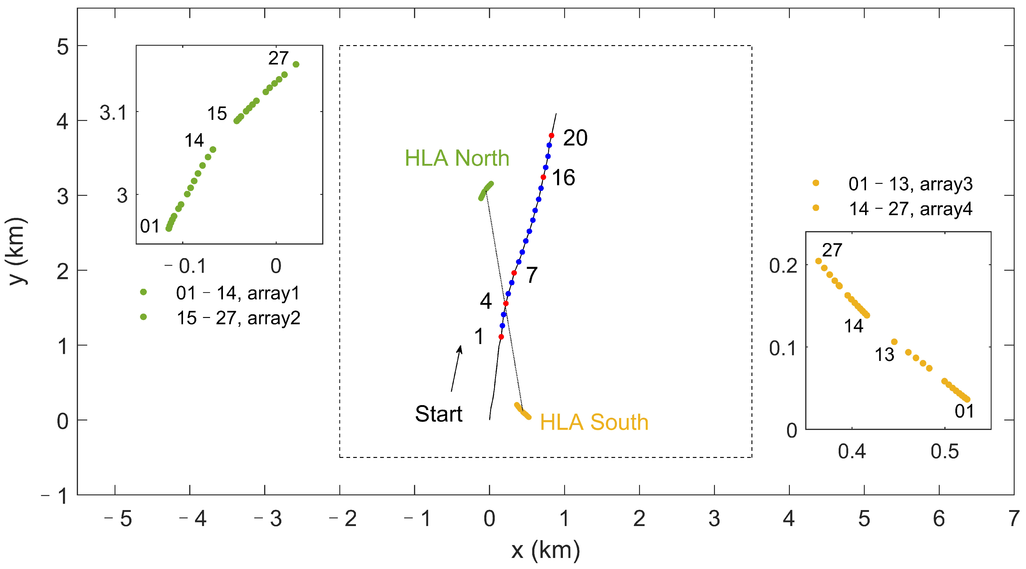
3. Application to Experimental Data

The SWellEx-96 horizontal array data set is obtained from the shallow water evaluation cell experiment which was conducted in May 1996, approximately 12 km from the tip of Point Loma near San Diego, California [19]. Two 32-element horizontal line arrays (HLAs), whose apertures are 255 m and 240 m respectively, were deployed on the sea bed of approximately 200 m depth, and 27 elements of each array are used in the processing. The distance between the two HLAs is approximately 3 km. The geometric plot of the 27-element subsets of the two HLAs and the source track for Event S5 are depicted in Figure 1. The inter-element spacing of the two 27-element HLAs varies significantly from 3.3 m to 43.5 m, and we divide the large array naturally into two small-aperture arrays to avoid overlarge inter-element spacing, which is also shown in Figure 1. Another advantage of subarray processing in such a scenario is that it can effectively mitigate the performance degradation due to the plane wave assumption. As is shown in [21], the propagation modeled by the normal mode solution to the wave equation is significantly different from a plane wave when the range from each hydrophone to the source varies across the array. Hence, when subarray processing is applied, the wave front can be approximately modeled by a plane wave since the range differences for the elements in a subarray are largely decreased from those of the previous large aperture array. In Event S5, two multi-tone acoustic sources were towed along a track between the two arrays, transmitting numerous tones between 49 Hz and 400 Hz. The two sources were towed at depths of about 54 m and 9 m, respectively, and the tow speed was 5 knots. In this section, the performance of the two typical DPD approaches GMA and N-MUSIC introduced in Section 2 is evaluated for the localization of the shallow source, and experimental results demonstrate the effect of the target–receiver geometry on the localization performance for coherent and non-coherent distributed systems.
A subset of data collected between 10 May 23:48:00 UTC and 11 May 00:07:00 UTC was processed, and a position estimate of the shallow source was obtained at the beginning of each minute. For the 19 minute duration, the source first approached the midpoint between the two HLAs and then proceeded away toward the endfire of HLA North, as illustrated in Figure 1. The nine tones transmitted by the shallow source were at 109, 127, 145, 163, 198, 232, 280, 335, and 385 Hz. A segment of duration 2.5 s data at the beginning of each minute sampled at 3276.8 Hz was first filtered at the tone frequency, and the appropriate SCMs were then formulated using the 8192 filtered time samples according to the array models. The 2D search area is [ 2 , 3.5 ] km along the x-axis, and [ 0.5 , 5 ] km along the y-axis with 10 m spacing.
The localization results of GMA and N-MUSIC with 198 Hz for the 20 segments processed are presented in Figure 2. It is noticed that GMA performs better than N-MUSIC for a long duration when the source moves away from the midpoint between the two HLAs (e.g., segments 7 to 15), where favorable source–receiver geometries are formed and the localization performance results of the two processors are very stable. The results validate the feasibility of the plane-wave-assumption-based DPD approaches in such an underwater scenario. In contrast, the estimation error varies significantly for the two processors when the source lies in between the two HLAs (e.g., segments 1 to 6). Equivalent performance is observed for the last 5 segments (16 to 20) when the source approaches the endfire of HLA North. We can see that the processors exhibit different characteristics with different source–receiver geometries. For better understanding of their performance, we divide the 20 segments into three sections as noted in Figure 2 based on the above observations, and then analyze the effect of target–receiver geometry and source frequency on the localization performance of the DPD approaches.

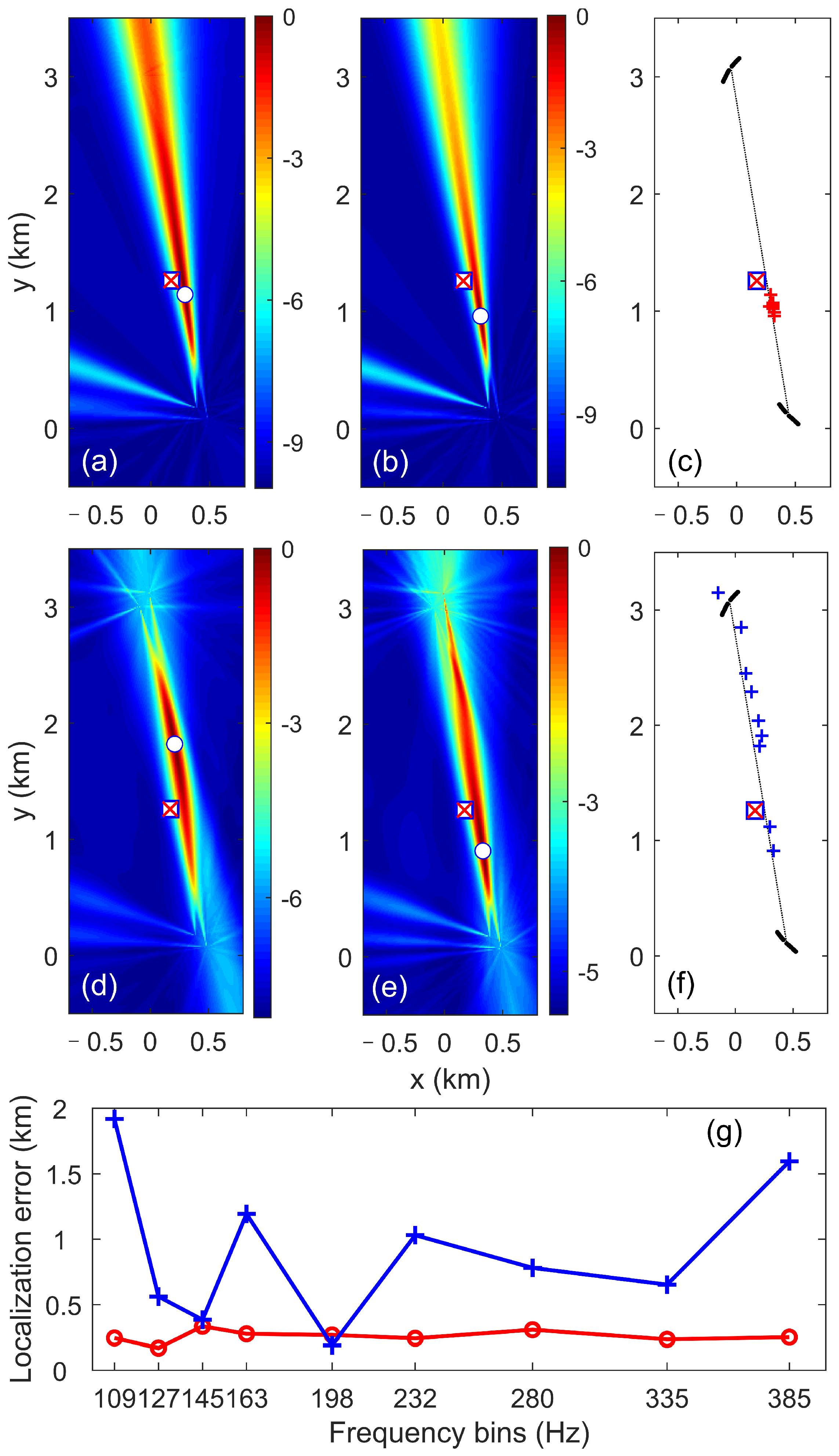
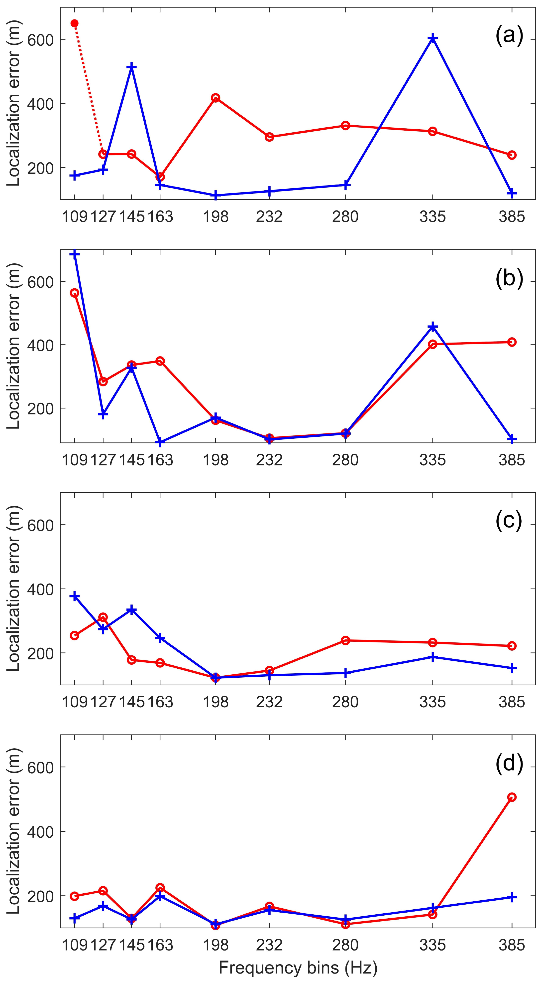
3.1. Section 1: Line Formation

Notice that the estimation error of the two processors does not display any “pattern” in the first section (segments 1 to 6) as it does in Section 2 and Section 3. In this process, the source–receiver geometry is poor since the source is approximately on the line connecting the center of each large HLA. The performance results of the processors are highly unstable and sensitive to the variation of the source–receiver geometry and source frequency. Let us firstly take segment 2 as an example to illustrate such instability with respect to the source frequency.
The localization results of GMA and N-MUSIC at segment 2 are displayed in Figure 3. At this segment, the source is almost on the line connecting the center of each HLA, and the source ranges to HLA North and HLA South are 1.8 km and 1.1 km, respectively. Observe that only “beams” from the two arrays in the south can been seen in the spatial spectrum of GMA, which form a very sharp intersecting angle, as the source is so close to the endfire of the arrays that the beam directions are almost the same. As the beams from the south arrays dominate the estimation process, the localization results of GMA with different frequencies are similar as shown in (c) and (g). In contrast to GMA, beams from all four arrays contribute to the N-MUSIC interference pattern, and they form a very large intersecting area almost covering the whole area between the two HLAs. It is shown in (f) that the estimated positions of N-MUSIC with the nine tones are widely distributed along the beams. As a result, N-MUSIC fails to obtain a correct position estimate with most of the tone frequencies, except with 145 Hz and 198 Hz when it “happens” to produce a location estimate that is relatively close to the true source position. Results indicate that when the source and receivers form a geometry with which the beams from the receivers are entirely overlapping, the estimate obtained by the non-coherent processor is not reliable and we have to resort to the global coherent processor for a stable estimate. We show in Figure 4 the 3D spatial spectrum of GMA and N-MUSIC. It can be seen that the beam power spreads along the y-axis and no peak is formed.
Next, we show in Figure 5 the sensitivity of GMA spectrum to source–receiver geometry, especially to the range difference between the arrays. As shown in Figure 2, the source ranges to HLA North at segments 3, 4, and 5 are 1.67 km, 1.52 km and 1.4 km, respectively, and ranges to HLA South are 1.3 km, 1.44 km, and 1.57 km, respectively. It is observed that GMA displays three different interference patterns as the range difference changes from 80 m to 370 m (note that the distance between the two HLAs is approximately 3 km). When the source is closer to HLA South at segment 3, beams from the south arrays dominate the interference pattern as shown in (a); when the source moves to segment 4, beams from the north arrays appear in the spectrum of (b); when the source is closer to HLA North at segment 5, beams from the south arrays disappear in (c). Actually, for most of the tone frequencies at segment 4, beams from the south arrays dominate the interference pattern, and only with 232 Hz can we see the presence of the north beams as shown in (b). In contrast, the spatial spectrum of N-MUSIC gradually shows an intersection pattern consisting of beams from all four arrays, and the intersection area becomes smaller as the source moves away from the midpoint between the two HLAs. For the purpose of clarification, we note here that when we say intersection pattern, we mean the intersection of beams from two or more widely distributed arrays. The beams from the two arrays in each HLA also intersect, but it is an exception since we divide a large-aperture array into two small-aperture arrays. Specifically, we process data at 17.5 s past segment 4, when the ranges to the two HLAs are 1488 m and 1490 m, respectively. This position is found by interpolating values between true source positions at segments 4 and 5 at the 2.5 s interval. Simulations with GMA show that when the range difference is almost zero, beams from the two HLAs form an intersection pattern like N-MUSIC for most of the tone frequencies, and the spectrum shown in (g) is an example with 232 Hz. This indicates that GMA depends largely on the array closest to the source in the localization task. Only when there exists another array that is equivalently close to the source will GMA demonstrate the intersection interference pattern, which is difficult to encounter in practical situations.
Figure 6 shows the localization errors of GMA and N-MUSIC at segments 3 to 5, as well as their errors at 17.5 s past segment 4. Results show that N-MUSIC achieves comparable or even higher accuracy than GMA when the source lies between the receivers but the beams are not entirely overlapping. We conclude that for the special source–receiver geometry where the source lies between the receivers, non-coherent processors are recommended since they demonstrate no worse performance than the global coherent processor and they are easier to implement in practical localization tasks. However, non-coherent processors become unreliable if the beams are entirely overlapping, and global coherent processing is the better choice.

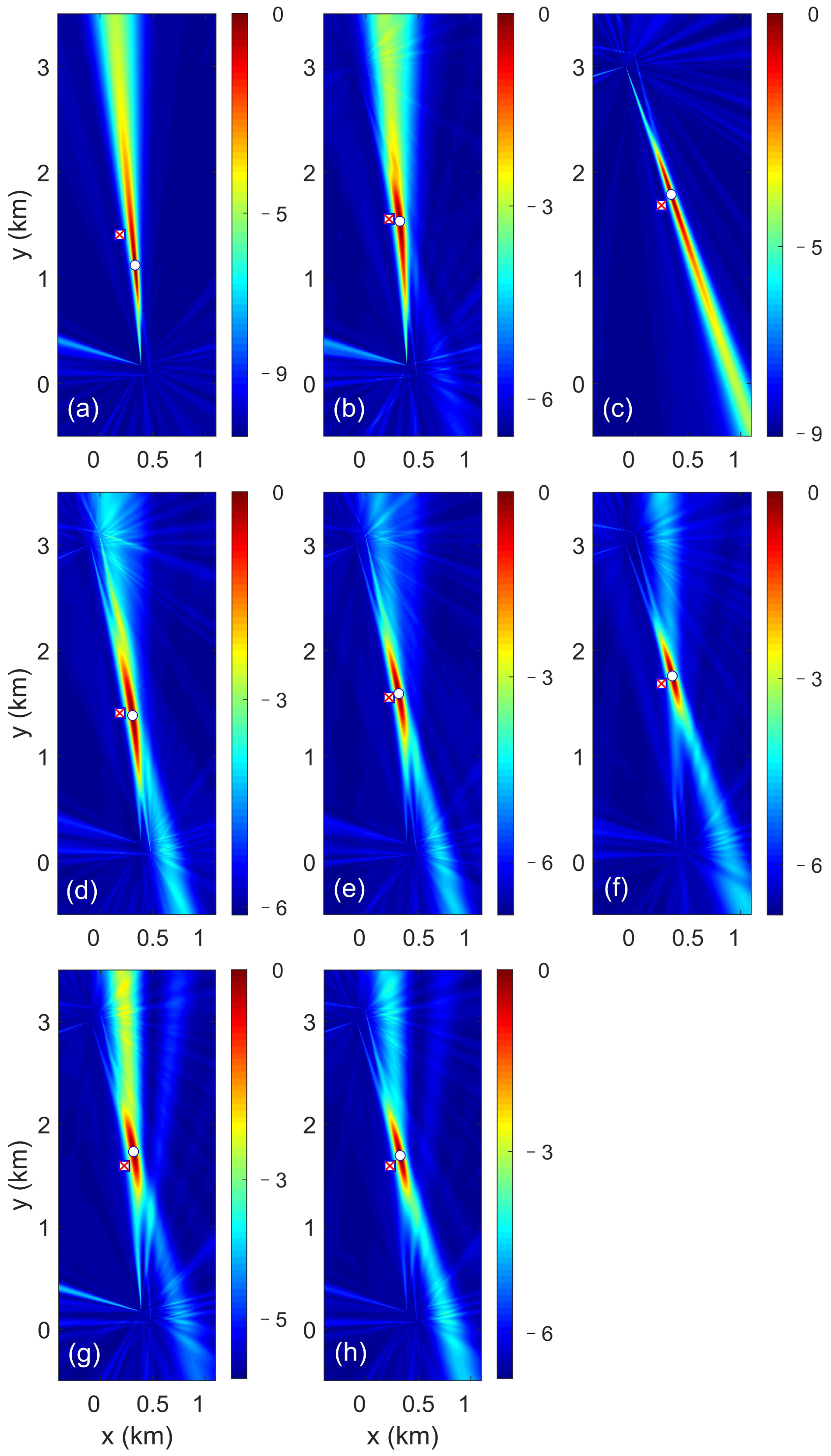
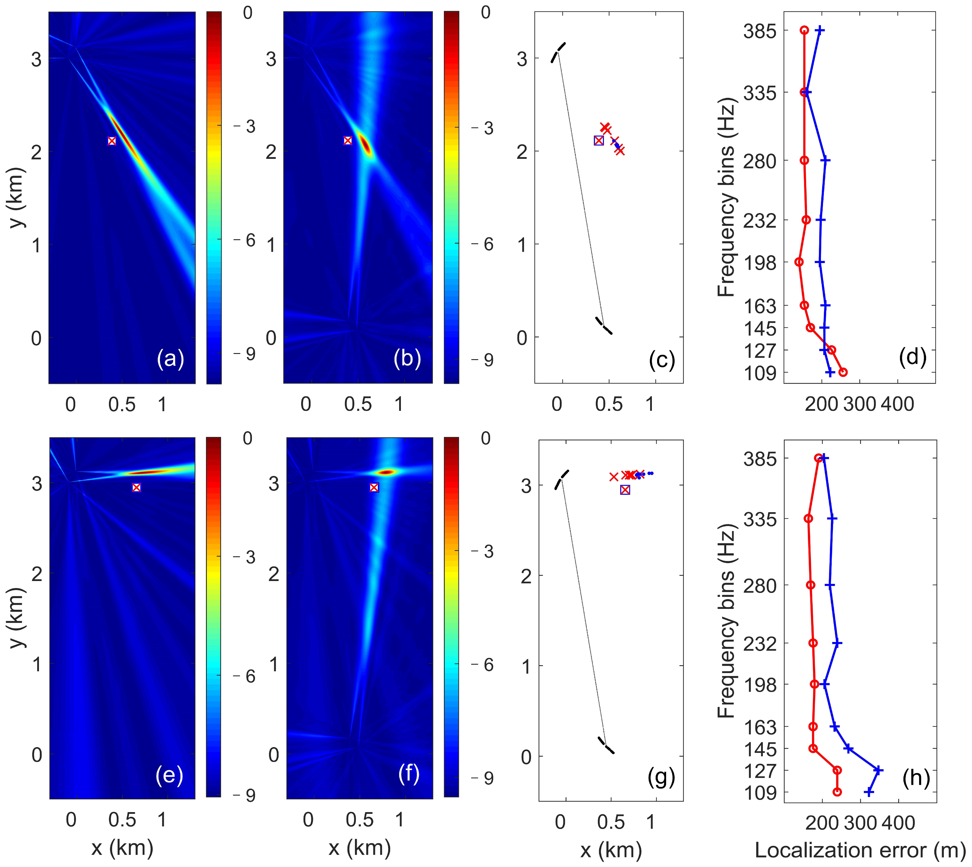
3.2. Section 2: Near-Broadside Formation

In Section 2 (segments 7 to 15), the source proceeded to the broadside of HLA North, and ended near its endfire. In this process, the source is getting closer to HLA North and away from HLA South, forming a favorable source–receiver geometry. It is observed that the localization performance of GMA and N-MUSIC is very stable in this duration as can be seen in Figure 2, where the estimation error has a slight increase as the source moves forward. Similar localization results are observed with the other eight frequencies. Localization results at segments 8 and 14 are presented in Figure 7 to show the typical behavior of GMA and N-MUSIC in this duration. Source ranges to the two HLAs at segment 8 are 1.04 km and 1.98 km, respectively, and at segment 14 are 0.71 km and 2.83 km, respectively. We can see that the beams from the two arrays in the north dominate the GMA spatial spectrum, and they form a clear intersection area as the source is at the broadside of the arrays. In contrast, the beams form a smaller intersection area for N-MUSIC with the help of the south beams, which, however, does not lead to better accuracy as shown in (d) and (h). We show in Figure 8 the 3D spatial spectrum of GMA and N-MUSIC. It can be seen that the beam power becomes more focused compared with Figure 4 and peaks are formed. In fact, GMA has the smallest estimation error for all 9 segments processed in Section 2. Notice that the position estimates are distributed along the direction of the north beams, which indicates that the north arrays produce stable beams, while the directions of the south beams vary with frequency. The deviation of the south beams results in larger localization error of N-MUSIC, but GMA adjusts inherently the contribution of the beams from different arrays to obtain better accuracy. This is an interesting and important property since the adjustment is realized by forming a coherent covariance matrix rather than through weights.
As can be seen in Table 1, when the source–receiver geometry is favorable (the source is at the broadside of the receivers and they form a triangle), non-coherent processors produce a good intersection pattern in the spatial spectrum. However, global coherent processors have better localization accuracy with the beams from the closest receivers dominating the interference pattern.

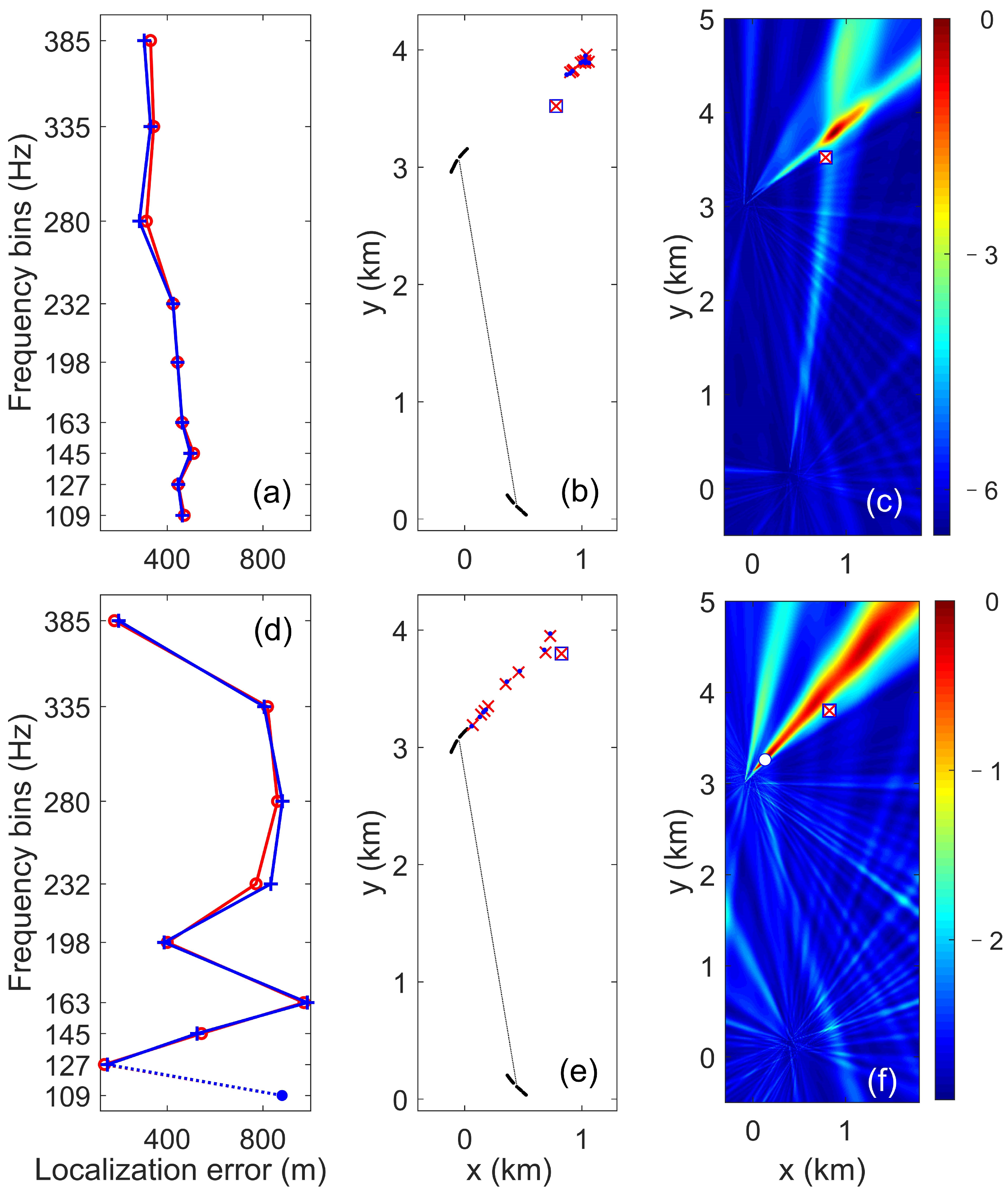
3.3. Section 3: Near-Endfire Formation

In Section 3 (segments 16 to 20), the source moved to the endfire area of HLA North. The source range to HLA North is about 1 km, while to HLA South it is larger than 3 km. Localization results of GMA and N-MUSIC at segments 18 and 20 are presented in Figure 9. The increase in error is obvious compared with the general cases in Section 2 (see Figure 7d,h), which is expected since source ranges to both HLAs are increasing. It is noticed that GMA and N-MUSIC exhibit similar accuracy with all tones. Actually, they produce similar interference patterns especially with lower frequencies. When the source is not exactly on the endfire of HLA North (e.g., segment 18), the processors produce a good intersection pattern and its performance is stable with different frequency tones. However, the power of the north beams is no longer concentrated when the source moves to segment 20, and we can see an ambiguity beam on the other side of HLA North. In this case, the estimation position is decided by the splitting narrow beams from the south arrays and the results are not liable any more.

3.4. Comparison between DPD and MFP

Next we compare the localization performance of the two DPD processors with the relative-amplitude MFP processor which achieves the best performance among the three multiple-array MFP processors presented in Tollefsen’s work [23]. For MFP processors, data were transformed to the frequency domain with 8192-point fast Fourier transforms (2.5 s time samples, Hamming windowed), yielding frequency bin widths of 0.4 Hz. To guarantee the same simulation setting where the previous results were obtained in Section 3.1, Section 3.2 and Section 3.3, SCMs were obtained with one snapshot on a certain frequency tone for both DPD and MFP processors. The 3D search volume for source positions is over (5.5, 5.5) km in (longitude, latitude) (50 m spacing) and 1–40 m in depth (2 m spacing).
Position estimates of the three processors in each section as well as their estimation errors are displayed in Figure 10. In Section 1, the position estimates of the three processors are all distributed along the line connecting the center of each HLA, but N-MUSIC has generally lower estimation errors. Results indicate that both DPD and MFP processors produce unstable and hence unreliable position estimates with such a geometry, but DPD processors demonstrate higher localization accuracy than the MFP processor. In Section 2, it is shown that the three processors have good and stable localization performance. GMA and the relative-amplitude MFP processor achieve similar accuracy, while N-MUSIC has larger estimation errors in this duration. This indicate that the spatial coherence of received signals between the arrays can be exploited to improve localization accuracy in this section. In Section 3, the estimation error of the three processors increases quickly as the source moves forward. The performance of the relative-amplitude MFP processor is very unstable (perhaps due to mismatch) when the source moves to the endfire of HLA North. Experimental results show satisfying performance of the MUSIC-based DPD processors with multiple horizontal arrays in shallow water when the SNR is high and the number of sources is known. However, their performance is not guaranteed when the number of sources (or the eigen-structure of the SCM) is difficult to estimate, and the plane-wave assumption may not hold in complex underwater environments.

4. Summary

In this paper, the effect of target–receiver geometry on localization performance, as well as on the exploitation of coherent and non-coherent bearing information is investigated by applying two DPD methods to the SWellEx-96 shallow water experimental data set. The global coherent processor GMA treats the receiving arrays as sub-arrays of a large array and exploits coherent bearing information. In contrast, the correlation between disparate arrays is considered unknown or irrelevant for the non-coherent MUSIC method, and hence non-coherent bearing information is used. Experimental results demonstrate the localization performance of the two processors with three different source-receiver geometries as the source moves along its track. The advantages and limitations of the exploitation of coherent and non-coherent bearing information in these scenarios are reported, which may provide some insights for the deployment of receivers in practical localization tasks.
The large-aperture arrays in the experiment are divided into two small-aperture arrays to mitigate the effect of plane wave assumption that may not hold for large-aperture arrays in ocean environments. Comparison between DPD and MFP processors demonstrates the feasibility of the DPD approaches in ocean acoustic environments as well as the credibility of the results in this paper. We would like to note here that DPD methods may not be practically implemented in real tasks since element-level received data are to be transmitted, but situational information can be deduced from the intersection pattern of the beams, which is very important for target localization tasks. The quality of the received data as well as the detecting information of the array may also be analyzed from the 2D or 3D spatial spectra, which is a very meaningful characteristic of direct localization methods.

Author Contributions

Conceptualization, L.W. and S.F.; methodology, L.W. and X.L.; writing—original draft preparation, L.W.; writing—review and editing, Y.Y. and X.L.; funding acquisition, L.W. All authors have read and agreed to the published version of the manuscript.

Funding

This research was supported in part by the National Natural Science Foundation of China under Grant No. 12204100, and in part by the State Key Laboratory of Acoustics, Chinese Academy of Sciences under Grant No. SKLA202205.

Institutional Review Board Statement

Not applicable.

Informed Consent Statement

Not applicable.

Data Availability Statement

The SWellEx96 shallow water experimental data set used in this study is publicly available at: http://dx.doi.org/10.6075/J0MW2F21 accessed on 22 November 2022.

Conflicts of Interest

The authors declare no conflict of interest.

References

  1. Nguyen, N.H.; Dogancay, K. Closed-Form Algebraic Solutions for Angle-of-Arrival Source Localization With Bayesian Priors. IEEE Trans. Wirel. Commun. 2019, 18, 3827–3842. [Google Scholar] [CrossRef]
  2. Wang, G.; Ho, K.C. Convex Relaxation Methods for Unified Near-Field and Far-Field TDOA-Based Localization. IEEE Trans. Wirel. Commun. 2019, 18, 2346–2360. [Google Scholar] [CrossRef]
  3. Wang, D.; Yin, J.; Zhang, T.; Jia, C.; Wei, F. Iterative constrained weighted least squares estimator for TDOA and FDOA positioning of multiple disjoint sources in the presence of sensor position and velocity uncertainties. Digit. Signal Process. 2019, 92, 179–205. [Google Scholar] [CrossRef]
  4. Weiss, A.J. Direct position determination of narrowband radio frequency transmitters. IEEE Signal Process. Lett. 2004, 11, 513–516. [Google Scholar] [CrossRef]
  5. Weiss, A.J.; Alon, A. Direct Position Determination of Multiple Radio Signals. EURASIP J. Adv. Signal Process. 2005, 2005, 37–49. [Google Scholar]
  6. Weiss, A.J.; Alon, A. A decoupled algorithm for geolocation of multiple emitters. Signal Process. 2007, 87, 2348–2359. [Google Scholar]
  7. Tirer, T.; Weiss, A.J. High Resolution Direct Position Determination of Radio Frequency Sources. IEEE Signal Process. Lett. 2016, 23, 192–196. [Google Scholar] [CrossRef]
  8. Tzafri, L.; Weiss, A.J. High-Resolution Direct Position Determination Using MVDR. IEEE Trans. Wirel. Commun. 2016, 15, 6449–6461. [Google Scholar] [CrossRef]
  9. Bosse, J.; Ferréol, A.; Germond, C.; Larzabal, P. Passive geolocalization of radio transmitters: Algorithm and performance in narrowband context. Signal Process. 2012, 92, 841–852. [Google Scholar] [CrossRef]
  10. Bosse, J.; Ferréol, A.; Larzabal, P. A Spatio-Temporal Array Processing for Passive Localization of Radio Transmitters. IEEE Trans. Signal Process. 2013, 61, 5485–5494. [Google Scholar] [CrossRef]
  11. Bishop, A.; Fidan, B.; Anderson, B.; Doğançay, K.; Pathirana, P. Optimality analysis of sensor-target localization geometries. Automatica 2010, 46, 479–492. [Google Scholar] [CrossRef]
  12. Moreno-Salinas, D.; Pascoal, A.; Aranda, J. Optimal Sensor Placement for Acoustic Underwater Target Positioning With Range-Only Measurements. IEEE J. Ocean. Eng. 2016, 41, 620–643. [Google Scholar] [CrossRef]
  13. Xu, S.; Doğançay, K. Optimal Sensor Placement for 3-D Angle-of-Arrival Target Localization. IEEE Trans. Aerosp. Electron. Syst. 2017, 53, 1196–1211. [Google Scholar] [CrossRef]
  14. Wax, M.; Kailath, T. Decentralized processing in sensor arrays. IEEE Trans. Acoust. Speech Signal Process. 1985, 33, 1123–1129. [Google Scholar] [CrossRef]
  15. Wang, L.; Yang, Y.; Liu, X. A distributed subband valley fusion (DSVF) method for low frequency broadband target localization. J. Acoust. Soc. Am. 2018, 143, 2269–2278. [Google Scholar] [CrossRef]
  16. Wang, L.; Yang, Y.; Liu, X. A Direct Position Determination Approach for Underwater Acoustic Sensor Networks. IEEE Trans. Veh. Technol. 2020, 69, 13033–13044. [Google Scholar] [CrossRef]
  17. Rieken, D.W.; Fuhrmann, D.R. Generalizing MUSIC and MVDR for multiple noncoherent arrays. IEEE Trans. Signal Process. 2004, 52, 2396–2406. [Google Scholar] [CrossRef]
  18. Wang, L.; Yang, Y.; Liu, X. A cluster-based direct source localization approach for large-aperture horizontal line arrays. J. Acoust. Soc. Am. 2020, 147, EL50–EL54. [Google Scholar] [CrossRef] [Green Version]
  19. Booth, N.O.; Hodgkiss, W.S.; Ensberg, D.E. SWellEx-96 Experiment Acoustic Data, UC San Diego Library Digital Collections. 2015. Available online: https://library.ucsd.edu/dc/collection/bb3312136z (accessed on 18 September 2019).
  20. Krim, H.; Viberg, M. Two decades of array signal processing research: The parametric approach. IEEE Signal Process. Mag. 1996, 13, 67–94. [Google Scholar] [CrossRef]
  21. Wilson, J.H.; Veenhuis, R.S. Shallow water beamforming with small aperture, horizontal, towed arrays. J. Acoust. Soc. Am. 1997, 101, 384–394. [Google Scholar] [CrossRef]
  22. Tollefsen, D.; Dosso, S.E. Source Localization With Multiple Hydrophone Arrays via Matched-Field Processing. IEEE J. Ocean. Eng. 2017, 42, 654–662. [Google Scholar] [CrossRef]
  23. Tollefsen, D.; Gerstoft, P.; Hodgkiss, W.S. Multiple-array passive acoustic source localization in shallow water. J. Acoust. Soc. Am. 2017, 141, 1501–1513. [Google Scholar] [CrossRef] [PubMed]
  24. Schmidt, R. Multiple emitter location and signal parameter estimation. IEEE Trans. Antennas Propag. 1986, 34, 276–280. [Google Scholar] [CrossRef] [Green Version]
  25. Gantmacher, F. Matrix Theory; American Mathematical Society: Providence, RI, USA, 1959; Volume I-II. [Google Scholar]
  26. Ferreol, A.; Boyer, E.; Larzabal, P. Low-cost algorithm for some bearing estimation methods in presence of separable nuisance parameters. Electron. Lett. 2004, 40, 966–967. [Google Scholar] [CrossRef]
Figure 1. (Color online) Geometric plot of the 27-element subsets of the two horizontal line arrays and the source track for Event S5. Filled green and yellow circles indicate the north large array (HLA North) and the south large array (HLA South), respectively. The four small-aperture arrays 1 to 4 are indicated by element indices. Dashed black line connects the center of the two HLAs. Solid black line indicates the source track for the first 30 min. Filled blue circles indicate true source positions for the 19 min data processed, and filled red circles mark several key points along the track. Dashed box indicates the 2D search area.
Jmse 10 01922 g001
Figure 2. (Color online) Localization results of GMA and N-MUSIC with 198 Hz for the 20 segments processed. (a) Position estimates of GMA (red cross symbols) and N-MUSIC (filled blue circles). Solid black line indicates true source track. (b) Range estimates of GMA to HLA North (red cross symbols) and HLA South (dotted red line with filled circles), and range estimates of N-MUSIC to HLA North (blue cross symbols) and HLA South (dotted blue line with filled circles). Solid green line and yellow line indicate true range to HLA North and HLA South, respectively. (c) Localization errors of GMA (solid red line with red circles) and N-MUSIC (solid blue line with plus symbols).
Jmse 10 01922 g002
Figure 3. (Color online) Localization results of GMA and N-MUSIC with nine tone frequencies at segment 2. (a,b) Spatial spectra of GMA with 127 Hz and 145 Hz. (d,e) Spatial spectra of N-MUSIC with 127 Hz and 145 Hz. True source position is indicated by red cross symbol inside the square. Estimated source position is indicated by white circle. (c,f) Position estimates of GMA (red symbols) and N-MUSIC (blue symbols) with nine shallow tone frequencies. (g) Localization errors of GMA (solid red line with red circles) and N-MUSIC (solid blue line with plus symbols).
Jmse 10 01922 g003
Figure 4. (Color online) 3D spatial spectrum of GMA (a) and N-MUSIC (b) with 127 Hz at segment 2.
Jmse 10 01922 g004
Figure 5. (Color online) (ac) Spatial spectra of GMA at segments 3, 4, and 5, respectively. (df) Spatial spectra of N-MUSIC at segments 3, 4, and 5, respectively. (g,h) Spatial spectra of GMA and N-MUSIC at 17.5 s past segment 4. Results are with 232 Hz. True source position is indicated by red cross symbol inside the square. Estimated source position is indicated by white circle.
Jmse 10 01922 g005
Figure 6. (Color online) Localization errors with nine tone frequencies at (a) segment 3, (b) segment 4, (c) segment 5, and (d) 17.5 s past segment 4 of GMA (solid red line with red circles) and N-MUSIC (solid blue line with plus symbols). Note that the estimation error of GMA at segment 3 with 109 Hz is 1681 m and is indicated by the filled circle in (a).
Jmse 10 01922 g006
Figure 7. (Color online) Demonstration of typical behavior of GMA and N-MUSIC in section 2. Results are with 198 Hz at segment 8 (first row) and segment 14 (second row), respectively. (a,e) Spatial spectra of GMA. (b,f) Spatial spectra of N-MUSIC. (c,g) Position estimates of GMA (red symbols) and N-MUSIC (blue symbols). True source position is indicated by red cross symbol inside the square. (d,h) Estimation results of GMA (solid red line with red circles) and N-MUSIC (solid blue line with plus symbols).
Jmse 10 01922 g007
Figure 8. (Color online) 3D spatial spectra of GMA (a) and N-MUSIC (b) with 198 Hz at segment 8.
Jmse 10 01922 g008
Figure 9. (Color online) Localization results of GMA and N-MUSIC at segment 18 (first row) and segment 20 (second row). (a,d) Localization errors with nine tone frequencies of GMA (solid red line with red circles) and N-MUSIC (solid blue line with plus symbols). (b,e) Position estimates of GMA (red symbols) and N-MUSIC (blue symbols). True source position is indicated by red cross symbol inside the square. (c,f) Spatial spectra of N-MUSIC with 280 Hz. Note that the estimation error of GMA and N-MUSIC at segment 20 with 109 Hz are 1728 m and 1750 m. They are indicated by filled red circle and filled blue circle in (d) respectively.
Jmse 10 01922 g009
Figure 10. (Color online) (ac) Position estimates of GMA (red symbols), N-MUSIC (blue symbols) and the relative-amplitude MFP processor (green symbols) for Section 1, Section 2 and Section 3, respectively. Solid black line indicates true source track in corresponding section. (d) Localization errors of GMA (red symbols), N-MUSIC (blue symbols) and the relative-amplitude MFP processor (green symbols). Results are with 198 Hz. Filled green symbols in (c) indicate the estimate with x value beyond this area. Filled green symbols in (d) on the dotted lines correspond to the estimates with error larger than 1 km.
Jmse 10 01922 g010
Table 1. Comparison of the DPD processors with three formations.
Formation TypeCoherent Bearing InformationNon-Coherent Bearing Information
Line formationClose array dominationLarge intersection area
Stationary localization resultsRandom localization results
Near broadsideClose array dominationClose array domination
Stationary localization resultsStationary localization results
Higher localization accuracyLower localization accuracy
Near end-fireClose array dominationMultiple intersection area
Stationary localization resultsDispersive localization results
Publisher’s Note: MDPI stays neutral with regard to jurisdictional claims in published maps and institutional affiliations.

