1. Introduction
Orthogonal frequency division multiplexing (OFDM) was developed from multi-carrier modulation technology and has the characteristic of anti-narrowband interference [
1]. The spectral efficiency of the communication process was improved by the adoption of overlapping sub-carrier modulation technology, which reduces the communication bandwidth. Because of these advantages, OFDM has become the preferred technical solution for high-rate underwater acoustic communication [
2]. As its name suggests, orthogonality between subcarriers can maximize the spectral efficiency and reduce inter-carrier interference (ICI) [
3,
4]. The presence of carrier frequency offset (CFO) in a communication system can destroy the orthogonality, which reduces the signal-to-noise ratio (SNR) and intensifies the ICI, significantly increasing the bit error rate (BER) of the received OFDM signal [
5]. Therefore, estimating and compensating for the CFO before demodulating and decoding the received signal is an important research objective for OFDM systems. Because of factors such as the sea surface fluctuation effect, turbulence, and internal wave motion, the transmitter and receiver terminals used in underwater communication usually have relative velocities, which leads to the Doppler effect. An approximate Doppler value is commonly estimated for each OFDM frame, and a resampling method is used for compensation after receiving the signal [
6]. Because the transmitted OFDM symbol is a wideband signal, there is a residual Doppler frequency shift in the system after resampling, which can be regarded as a result of the CFO [
7].
Presently, the methods used for CFO estimation can be mainly divided into two categories [
8,
9]: data-aided estimation [
10,
11,
12] and non-data-aided estimation [
13]. When the data-aided estimation is performed in the time domain, it utilizes a training sequence [
10], whereas if it is performed in the frequency domain, it uses pilot symbols [
11,
12,
14]. The non-data-aided estimation methods are also commonly referred to as blind estimation. Some auxiliary information about the received signal is used for blind channel estimation, but this does not increase the overhead of the channel resources. This information usually includes pre-set structures and characteristics such as the cyclic prefix (CP) in OFDM [
15,
16,
17,
18], responses on the null subcarrier [
19,
20,
21], constant modulus [
22,
23,
24], and non-Gaussianity of modulated signals [
25]. In addition to the blind estimation method, Li et al. proposed that OFDM with ICI could be regarded as a multi-carrier-code division multiple access (MC-CDMA) system on the receiver side [
26] because MC-CDMA is a technology that combines OFDM and code division multiple access (CMDA). Moreover, the ICI matrix in OFDM is an orthogonal matrix. An
ICI matrix acts as a spreading code matrix; thus
N data symbols in the OFDM are spread over all
N subcarriers in the MC-CDMA system [
26]. The data symbols quantize the normalized CFO, obtaining M spreading code matrices as candidates. The received signal is then decoded, decided, and reconstructed using candidates. The Euclidean distance is utilized to measure the difference between the reconstructed and received signals. The result with the smallest difference value corresponds to the best-normalized CFO estimation. The scheme should be able to perfectly cancel the ICI caused by the CFO. In 2013, a joint estimation method for the CFO and channel information that embedded the channel estimation block was proposed on the basis of previous work [
27]. Concurrently, the computational complexity was also improved by adopting the “golden section search” [
28]. Simulation results showed that the proposed scheme achieved a promising performance, which was comparable to that of OFDM in the absence of ICI.
Although much research is available in the literature related to CFO estimation and compensation, few schemes have been presented for time-varying CFO (TVCFO) estimation in underwater acoustic communication. Based on the above analysis, relative motion causes a Doppler effect or CFO, and a constant CFO can only be caused by a relatively uniform motion. However, in a complex and changeable underwater environment, it is difficult to guarantee a relatively uniform motion. Instead, an unpredictable acceleration often exists, which leads to a TVCFO in OFDM. This TVCFO is very difficult to deal with because its tracking and equalization usually require high computational complexity [
29], which tends to increase linearly with the number of symbols in the OFDM frame. An introduction to the existing research is given below.
Mason et al. proposed a method for estimating the constant Doppler shift or slowly changing the time-varying Doppler shift within the packet by transmitting two identical OFDM symbols and employing a bank of parallel autocorrelators at the receiver [
30]. This work was extended by Parrish et al. [
31], who suggested tracking the Doppler variation with the help of marginal maximum likelihood estimation between symbols. Carrascosa et al. [
32] proposed a TVCFO estimation method that predicted and tracked the nonuniform Doppler shift between adjacent data blocks based on the frequency and time correlation. Abdelkareem [
29] assumed that the Doppler shift varied linearly among OFDM symbols, based on the principle that a Doppler shift changes the signal length in the time domain. This requires frequent sampling and interpolation to estimate and compensate for the Doppler shift within the duration of a symbol. Simultaneously, the first-order statistics of the cyclic prefix are also estimated to reduce the ICI. In 2016, Abdelkareem studied the effect of sudden changes in the acceleration and velocity directions on the cyclic prefix correlation and proposed an adaptive time-varying Doppler estimation scheme. This adaptive mechanism was embedded in the automatic selection of the best estimation method based on CP window center positioning, first-order expectation, and autocorrelation of the CP [
33]. Avrashi first studied the closed-form expression of the received signal that passed through a double-spread channel based on the least squares criterion. The value of the constant CFO was obtained using a root-based and eigenvalue decomposition-based CFO estimator [
25]. In 2022, Avrashi extended the constant CFO to a polynomial and piecewise model variation over time [
9], and implemented a method for estimating the TVCFO based on previous research. Compared with a grid search, which imposes a high computational burden on a modem [
33], heuristic-based intelligent optimization algorithms have remarkable advantages, including greater adaptability and higher solution efficiency [
34]. Therefore, they have allowed great progress in channel estimation [
35,
36,
37,
38,
39].
The differential evolution (DE) algorithm is a prevalent example of intelligent optimization algorithms. It has a simple structure with few parameters, but exhibits excellent performance [
35,
37]. The DE algorithm has a feature that distinguishes it from other intelligent optimization algorithms: it is especially suitable for solving problems where there are dependencies between the adjacent variables to be optimized [
40,
41]. The dependencies refer to the fact that variables are linked by a similar influencing factor, such as Rosenbrock, Schaffer F7, and Whitley’s composite functions in the benchmark suites. Coincidentally, underwater acoustic channel conditions do not change suddenly under normal circumstances. Even when the CFO changes over time, the CFO value on a subsequent block changes on the basis of the previous CFO value in terms of the OFDM structure. In other words, time-varying CFO estimation for OFDM systems falls squarely into the category of problem optimization with adjacent variables depending. In summary, the specific mutation and crossover operations of the DE algorithm can be used to track the time-varying CFO values of adjacent blocks in an OFDM data frame. After a limited number of iterations, the best estimate of the time-varying subcarrier frequency offset can be obtained.
From the literature, an OFDM model analogous to the MC-CDMA system can realize perfect ICI cancellation without losing any system overhead [
26,
27]. Considering the significant advantages and development potential of this scheme in underwater acoustic communication, we extended the model to time-varying environments and obtained a TVCFO estimation and thus compensation in this study. Simultaneously, the crossover characteristic of the DE algorithm was used to track the TVCFO and obtain the best estimation values based on its strong optimization ability. Specifically, the CFO value of each block was regarded as a variable to be optimized in the DE. The spread code matrix in the MC-CDMA system was obtained based on the variables by analogy, and then the received signal was reconstructed using the estimated CFO values. The Euclidean distance between the reconstructed and received signals was used to form the cost function. The optimal estimation of the TVCFO was achieved by the iterative use of the genetic operators of the DE.
The objective of this investigation was to study the performance of time-varying CFO estimation in OFDM systems based on the DE algorithm due to its advantages in solving problems with adjacent variables depending. The main contribution of this paper is to provide a feasible idea for time-varying CFO estimation, and the proposed method not only has the general applicability of modulation methods but also can improve the noise tolerance in demodulation. The remainder of this paper is organized as follows:
Section 2 introduces the OFDM system model and DE.
Section 3 details the proposed OFDM TVCFO estimation methods. The results and discussion are presented in
Section 4. Finally, we conclude this paper and make suggestions for future research in
Section 5.
3. Time-Varying Carrier Frequency Offset Estimation
The previous section discussed a model OFDM system with ICI caused by the CFO, which was analogous to the orthogonal MC-CDMA was discussed. However, because of the complexity of underwater acoustic environments, it is inappropriate to assume that both transducers will maintain uniform motion over a long period. Their motion can be impacted by multiple factors, including sea surface undulation, turbulence, and internal wave motion. More often, this relative motion is a variable speed motion with random accelerations. Therefore, the ICI in the received OFDM signal has a TVCFO rather than a constant CFO. In general, the duration of one OFDM block of underwater acoustic communication lasts from tens of milliseconds to approximately one hundred milliseconds. Considering the actual environment for underwater acoustic communication, we can reasonably assume that the acceleration of the relative motion is constant over the duration of an OFDM block; that is, the CFO changes within the duration of an OFDM frame but remains constant in the very short OFDM time block. Therefore, the model mentioned above should be modified slightly to change the constant CFO in the frame time to a variable value, while allowing it to remain steady during the block duration. The estimation of a single CFO value within a data frame is changed to finding the CFO values for each block within a data frame.
Water works as a waveguide in communication; however, it is also a viscous fluid, making it impossible for channel conditions to change quickly. Therefore, there are dependencies between the CFO values in neighboring blocks of the received signal because the velocity of relative motion corresponding to the latter time block changes based on that of the previous time block, which is adjacent to it. As previously mentioned, relevant research has shown that the DE algorithm is particularly suitable for dealing with problems in which there are dependencies between the adjacent parameters to be optimized. Therefore, we used the DE algorithm to jointly optimize the estimated TVCFO values in each block of the received signal. Based on the above analysis, the specific steps for estimating the TVCFO using the DE algorithm are given below.
- (1)
Determine optimization variables and their limits
Based on the previous analysis, this study investigated TVCFO estimation, where the CFO values on multiple OFDM symbol blocks varied over time and were unequal. The CFO on each OFDM symbol in a frame can be regarded as a variable to be optimized. If a data frame has
N symbol blocks, then the
th individual of the DE can be expressed as follows:
for
, where
is the population size of the DE. According to the introduction of Formula (
3), the normalized CFO is in the range of [0, 1]. In other words, the minimum value,
, is 0, and the maximum value,
, is 1. If it exceeds the limit, it should be readjusted back to this range; otherwise, it is meaningless. Real number DE coding was adopted in this study.
- (2)
Determine the fitness function
The fitness function can generally be regarded as a cost function in an optimization problem or its equivalent transformation and is mainly used for measuring the quality of solutions. For minimization problems, a smaller fitness function value indicates a higher quality for the individual solution. When the fitness function value is zero, the solution has the highest quality, and the individual is therefore the optimal solution. When the optimal solution was introduced and the Euclidean distance between the reconstructed and received signals was zero, the estimated value of the CFO was the actual value of the received OFDM signal. Although the fitness value could not be zero because of the influence of noise, there was still a relationship between the quality of the solution and its fitness. A smaller fitness value indicated that the estimated value of the CFO was closer to the real value. Because the TVCFO was considered, it was necessary to take the overall performance of the CFO values on all the symbol blocks within an OFDM frame into account. Hence, the mean value of the reconstruction differences was employed as the fitness value:
where
denotes the vector of the estimated CFO values on each block.
- (3)
Initialize the population
The initial population,
, consists of
original individuals, which are randomly generated in the decision space constrained by the upper and lower bounds of each dimension:
Thus
can be expressed as follows:
for
. In addition, the fitness value of the population can be obtained by substituting the initial population into the fitness function (
12).
- (4)
Perform genetic operations:
Populations are sorted based on the fitness values in the typical method before performing genetic operations. The sorting operation is used to facilitate the mutation operator to make full use of promising individuals with high quality because a solution with higher quality is the individual that carries more useful information. In other words, these individuals can accelerate the convergence and guide the population to find the optimal solution faster.
After completing the sorting operation, the mutation operation is performed. This operation can be expressed by the following formula:
where
is the mutation vector corresponding to the
i-th target vector,
.
is a promising individual selected from the top
of the current population. Individual
is randomly selected from the current population, while individual
comes from the union of the current population and these obsolete individuals, which can increase the diversity and prevent mutation vector
from falling into the local optima. These vectors differ from each other. Mutation factor
, which usually lies in the range of [0, 1], is used to scale the difference vector. Here,
g represents the
g-th generation of genetic operations.
Following the mutation, an exponential crossover operation is performed on mutation vector
and objective vector
to further increase the diversity of the current population. Specifically, integer
r is randomly selected from [1,
N]. This integer acts as the starting point of the offspring vector, from which it is exchanged with the components of the mutation vector. Another integer
L limited by [1,
N] is used to determine the dimension proportion of the offspring inherited from the mutation vector.
L can be determined using the following pseudocode:
Crossover rate
is a parameter that controls the value of
L. After parameters
r and
L are determined, the offspring vector can be obtained as follows:
where
is an operation that obtains the remainder. Next, the offspring are evaluated.
Lastly, the selection operation is executed. For a minimization optimization problem, the individuals with lower fitness values in the parents and offspring survive to the next generation. Then, a new population is obtained. The selection operation is as follows:
where
represents the fitness value of the corresponding vector, (i.e., the function value of the cost function);
represents the offspring individuals; and
represents the parent individuals.
- (5)
Judge termination conditions
There are two main types of termination conditions: when the error accuracy of the best solution reaches a pre-set value and when the maximum iteration number meets a pre-set value according to the computing complexity. If the termination conditions are met, the individual corresponding to the best quality is output as the optimal solution in this loop. Otherwise, the execution is repeated from step 4 until the termination conditions are met.
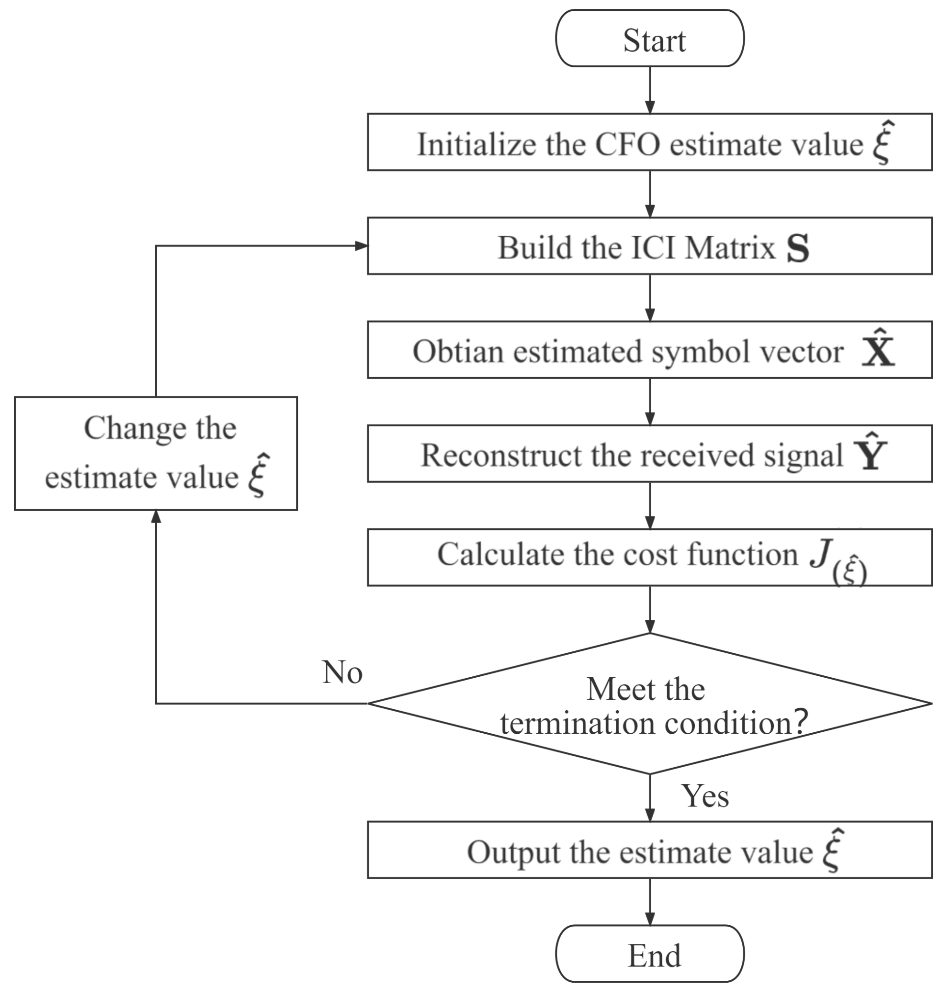
Algorithm 1 presents the pseudocode of the proposed DE-aided TVCFO estimation.
| Algorithm 1: Pseudocode of the proposed scheme |
Step 1 Initialization Set population size , dimension N, maximum generation number , and generation counter . Then initialize the original population with uniformly distributed in the limits, and evaluate the original population. Step 2 Evolution Iteration WHILE ( g ≤ ) DO Step 2.1 Preparation Sort current population according to the fitness values; Step 2.2 Mutation Operation Determine the value of mutation factor ; Perform the mutation operation according to ( 15); Step 2.3 Crossover Operation Determine the crossover rate in the type of exponential crossover; Execute the crossover operation based on ( 17) to obtain the offspring; Step 2.4 Selection Operation Substitute the offspring into ( 12) and get the fitness value; Carry out the selection operation according to ( 18); Step 2.5 Update the Generation Counter Increase the generation counter by 1, that is ; END WHILE Step 3 Output the Solution Solution with the smallest fitness value is output as the best TVCFO estimation. |
4. Results and Discussion
This section first describes a simulation experiment that used the proposed method for TVCFO estimation. Then the results are analyzed. To verify the suitability of using DE to estimate the TVCFO in an OFDM system, it was compared with representative intelligent optimization algorithms applied to channel estimation (the genetic algorithm (GA) [
39] and Simulated Annealing Mutated-Genetic Algorithm (SAMGA) [
36]) on the same model. We gathered the statistics and results of the proposed scheme, as well as the received signal with and without the actual TVCFO compensation, using the bit error rate (BER). Finally, the performances of the proposed scheme for four different modulation types were examined given to test its universality.
An OFDM system with eight blocks in one frame was considered. Each block contained
subcarriers. Binary phase-shift keying (BPSK) modulation was adopted if there was no additionality specified. A channel fading diagonal matrix was obtained based on the channel impulse response, as discussed in [
33] (i.e.,
) [
33]. Two different types of TVCFO were considered for simulation analyses i.e., fourth-order polynomial function and sinusoidal function [
9]. One of the CFO variations was a fourth-order polynomial function (
19):
where
are uniformly distributed and randomly taken from the limits of
, that is
, and
K is the number of blocks. The other variation form was the sinusoidal function (
20):
where
and
. The limits of the TVCFO estimation values were modified as [−0.5, 0.5] for convenience.
4.1. Results of Different Estimators
Based on a model where the received OFDM signal with ICI caused by the TVCFO was analogous to the orthogonal MC- CDMA system, the estimation was conducted using DE. To verify its suitability for considering the dependencies between the CFO values in adjacent blocks of the OFDM data frame, the performance of the DE algorithm for the TVCFO estimation was compared with those of the SAMGA [
36] and GA [
39], which are frequently used in channel estimation. The parameters of the DE algorithm used in this study were consistent with those in [
42], and the parameters of the compared algorithms were set to the values reported in the original papers.
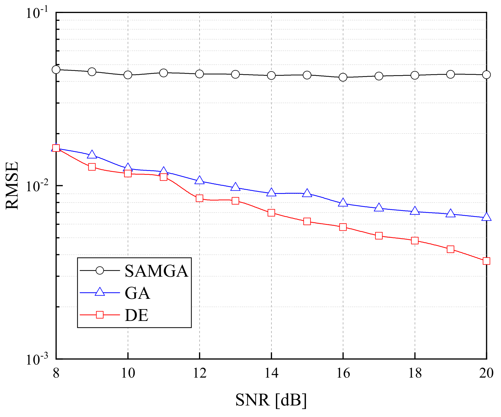
Figure 2 shows the performances of the DE algorithm, GA, and SAMGA when estimating the TVCFO in the form of a polynomial function with the same computing resources. The data in the figure are the averages obtained from 50 independent runs under different SNRs, as are the data in the following figures. The measurements show the Root-Mean-Square Error (RMSE) of the CFO values on the OFDM blocks, which can be defined as follows:
The black, blue, and red curves represent the results obtained by the SAMGA, GA, and DE estimators for the improved model, respectively. The RMSE values improved as the SNR increased. However, the SAMGA did not improve the performance of the genetic algorithm in this case. It was inferred that this lack of improvement was a result of the limited computing resources, which made the large population size unsuitable. Moreover, the SAMGA increased the diversity to prevent premature, which also wasted computing resources. Generally, the available time resources are seriously constrained in underwater acoustic communication. Therefore, the advantages of the SAMGA could not be fully utilized. The GA had a remarkable performance compared to that of the SAMGA; However, the performance of the DE algorithm was slightly better than that of the GA. The average RMSE value with the DE algorithm was approximately
smaller than that of the GA when the SNR was less than 12 dB. When the SNR exceeded 12 dB, the average RMSE of the DE estimator increased, becoming
smaller than that of the GA estimator, and finally reaching a peak that was
lower at 20 dB. This significant improvement was due, not only to the adaptive parameters of the DE algorithm used in this study [
42], but also to its advantage when solving problems with dependencies between adjacent variables. The GA could not compete with the DE algorithm in terms of the dependencies between adjacent variables which is the pivotal characteristic of TVCFO estimation. The above analysis was confirmed by the gap between the two curves becoming progressively obvious as the SNR increased. Because the amplitude of the noise followed a normal distribution and had significant randomness, the dependencies between adjacent variables were diluted. However, as the SNR increased, the influence of the noise decreased, and the connections between adjacent TVCFO values could be more easily mined by the DE algorithm.
The best results of the three estimators were substituted into the improved system model for demodulation. The BER values were determined based on the demodulation results, and are summarized in
Figure 3. According to the curve, when the SNR did not exceed 13 dB, the performances of the three estimators were comparable, and it may be inferred that their accuracies were acceptable. Under the condition of a low SNR, the source of the error values was mainly the noise, and the CFO estimation bias was relatively negligible. The difference between the three estimators becomes clear from the results at 14 dB. When the SNR is less than 17 dB, the performance of the SAMGA estimator is comparable to those of the GA and DE estimators. After the SNR exceeds 17 dB, the SAMGA with the lowest estimation accuracy shows the worst demodulation performance. The comparison between GA and DE algorithms fluctuated, which was a result of the combined effect of noise and the CFO estimation accuracy. The noise uncertainty led to a performance undulation with the same SNR for both estimators. With an increase in the number of result statistics or SNR, the gap between the DE and GA estimations became apparent, as was evidenced by the results at 20 dB.
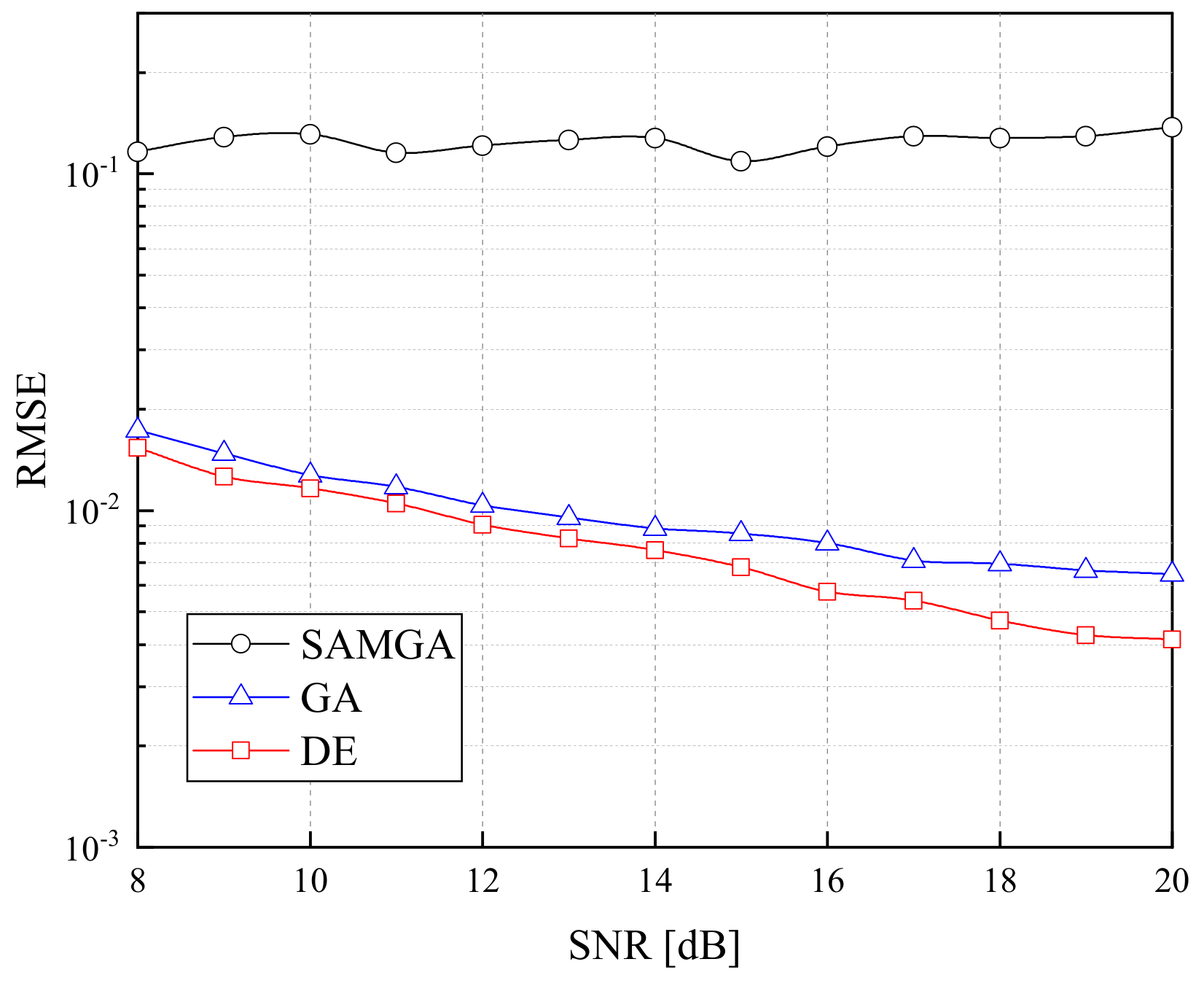
The results of the three algorithms when the CFO values varied in the form of a sinusoidal function with the same computing times are shown in
Figure 4. By comparing the data in
Figure 2 and
Figure 4, similar conclusions can be drawn: the estimation accuracy of the DE algorithm was significantly better than those of the SAMGA and GA. The mismatch between population size and mutation operation adopted by the SAMGA for the TVCFO estimation caused it to have the worst performance of the three estimators. In addition, it should be noted that for the SAMGA estimation, the RMSE of the CFO value with the sinusoidal function was roughly an order of magnitude worse than that in the polynomial function. The difference in the estimation accuracy also led to distinct demodulation results. As seen by the BER statistics for the SAMGA estimator in
Figure 5, the demodulation results were almost unacceptable because of the large deviation in the CFO estimation. Additionally, the CFO estimation bias of the SAMGA estimator fluctuated very little for different SNRs. Therefore, the BER improvement seen in
Figure 5 came merely from the increase in the SNR. The BER curves for the GA and DE estimators further corroborated the conclusions we drew above: the demodulation performances of the DE and GA estimators were dominated by the SNR in the cases with low SNRs, whereas under high SNR conditions, the quality of the TVCFO estimation was reflected in the BER results. The RMSE of the DE estimator was
smaller than that of the GA estimator when the SNR was 20 dB, which corresponded to a
improvement in the BER after demodulation. Based on an analysis of the results of the simulation experiments with the three estimators using two different variations of CFO values, we can safely conclude that, because the dependencies between adjacent variables were considered by the DE algorithm and not the other intelligent optimization algorithms (the GA and SAMGA), it would be appropriate to use the DE algorithm to estimate the TVCFO in underwater acoustic communication.
4.2. Results of Demodulation with/without Compensation
To further verify the performance of the DE estimator of the TVCFO, the demodulation results with and without CFO compensation and with DE estimation value compensation are given in
Figure 6. In this figure, the black solid line with a circle represents the demodulation results for the OFDM system model without compensation. The blue dashed line which is marked as “OFDM without TVCFO” shows the demodulation results in the absence of the CFO, which is equivalent to compensation with real CFO values. And the red squares marked as “OFDM with TVCFO compensation” show the demodulation results when using the DE estimation values. The BER without compensation was much higher than that with compensation, which was predicted. Surprisingly, the results of the compensation with the estimated values were highly coincident with the results when there were no CFO values. Moreover, the demodulation results for the CFO compensation with DE estimation were better than those without the CFO when the SNR is equal to 20 dB. The only possible reason for this was the influence of noise. According to (
7) and (
8), the reconstructed signal could be used to directly calculate the cost function with the actual received signal without considering the noise. Therefore, the effect of noise on the demodulation performance was converted into the CFO on each OFDM block by the DE estimator and taken into account in the simulation values.
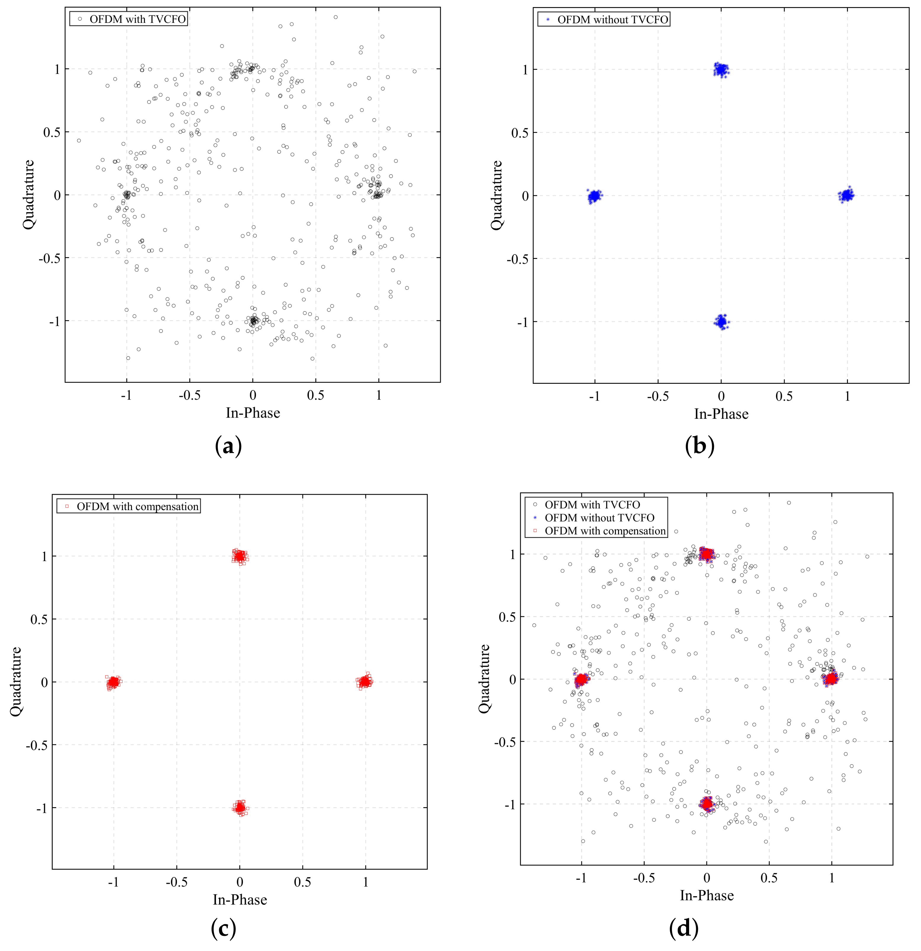
Figure 7 shows a constellation map after demodulation in the three cases: without the CFO compensation, with the actual CFO compensation, and with the DE estimation value compensation. The CFO values that varied as a sinusoidal function were adopted in these simulations. The received data without CFO compensation were randomly distributed, which resulted in difficulties in making the correct decision. In the case of the compensation with the DE estimation values, the data surrounding the correct constellation points were well organized. Importantly, the data boundaries were very clear, because valid decisions could be easily made. In addition, these data were highly coincident with the compensation results with the actual CFO values. Specifically, there is significant overlapping between the red square and blue star data in the figure. This phenomenon demonstrates the validity of the proposed scheme for estimating TVCFO values.
4.3. Results of Different Modulations
Finally, we used the proposed scheme with four modulation methods to investigate the performance in terms of its universality. The BER values of the demodulation results were calculated and are shown in
Figure 8. The four different modulation methods were BPSK, quadrature phase-shift keying (QPSK), differential QPSK (DQPSK), and 16-bit quadrature amplitude modulation (16QAM). According to the data, the demodulation results with 16QAM were similar to those of the QPSK cases analyzed above. The DE algorithm was used to estimate the CFO value for each OFDM block before the received signal was compensated with the values. A comparison of the curves shows that its demodulation was significantly better than the case of direct demodulation without compensation. Moreover, the compensation results with the DE estimated values were consistent with those obtained using actual CFO values. This means that the actual TVCFO value could be obtained using the DE estimator. In the case of BPSK, the DE algorithm with estimation value compensation performed better than that without the TVCFO, which was clear in the high SNR situation. This was because there was less pressure to make a correct BPSK judgment compared to QPSK with the same estimation accuracy, which was affected by the fewer decision options of BPSK. The effect of noise on the OFDM block was considered to be part of the CFO. Therefore, the possibility of a mismatch was smaller because BPSK has fewer decision options. This was also the reason that the demodulation results based on the estimated values were slightly better. For DQPSK, the demodulation effect of the DE estimated values were worse than that of the compensation executed using the actual CFO values, which was also due to the effect of noise being regarded as carrier frequency deviation. Phase changes on adjacent subcarriers are employed to transmit information in the DQPSK modulation. However, the original information is destroyed by the equivalent CFO introduced when dealing with noise in the DE estimator. Therefore, the demodulation results deteriorated with the compensation of the actual TVCFO values. In general, it was relatively acceptable to use the DE algorithm to estimate the TVCFO in DQPSK. In summary, the TVCFO estimation using the DE algorithm was very effective in the PSK and QAM modulation modes. Although the performance of the DE algorithm in the DQPSK modulation mode was not the same as those with the PSK and QAM, the demodulation result after compensation based on the estimated value is significantly better than that without compensation. Moreover, as the SNR increases, the gain after compensation is also more obvious.
This section showed how three estimators (the SAMGA, GA, and DE algorithms) were adopted for the TVCFO estimation on the improved OFDM model. A comparison of the results in terms of the RMSE of the estimated values and the BER of demodulation showed that the mechanism of the DE algorithm, which considers the dependencies among adjacent variables, was very suitable for solving the TVCFO estimation problem. The demodulation performances for the received signal without compensation, with actual CFO values, and with estimated values obtained by the DE compensation were determined. The results demonstrated that the proposed scheme could achieve real TVCFO values, and the effect of noise on the demodulation could also be considered in the QPSK modulation. Ultimately, the performances of the DE estimator with four modulation schemes, BPSK, QPSK, DQPSK, and 16QAM, were tested. The proposed scheme correctly estimated the TVCFO values under the QPSK and 16QAM modulation. The performance under BPSK modulation was the best of the four, and it was easier to reduce the influence of noise under a high SNR. The DQPSK modulation was not as promising as the other three modulations. However, the results were also acceptable, and the DE estimator could be utilized with DQPSK and can be worked as a candidate.


