Structural Prediction Analysis of Cross-Sea Cable-Stayed Bridges during Operation Based on Existing Traffic Volumes

Abstract

In order to study the safety state of the structure of a cross-sea cable-stayed bridge during its operation period, this paper proposes a combined long-term traffic prediction model based on the XGBoost (eXtreme Gradient Boosting) model and LSTM (Long Short Term Memory) model in the context of a cross-sea cable-stayed bridge in Qingdao. XGBoost is an optimized distributed gradient enhancement library. LSTM is a neural network for processing long sequence data. The LSTM model and the XGBoost model were first built separately, and then a genetic algorithm was used to select the optimal weight parameters to combine the two models for prediction. Based on the traffic prediction results of the combined LSTM-XGBoost model, a finite element model was established using numerical analysis. The effect of different traffic volumes on the deflection and stresses in the span of the main beam and the stresses in the diagonal cables was analyzed using the time course analysis method. From the point of view of structural safety, the maximum of future traffic limits and more reasonable average traffic speeds are given to provide a basis for the later management of the bridge.

1. Introduction

With the rapid development of China’s economy, the transport industry and the automotive industry have developed rapidly. The speed and level of construction of urban bridges as an important part of road traffic has developed rapidly. The volume of traffic on bridges during urban operation increases significantly as the economic level of a city rises, seriously increasing the load burden on bridges and having a serious impact on their safety and service life. The dramatic increase in traffic will directly cause damage to the bridge structure during operation, weakening the durability of the structure and, to varying degrees, reducing the bridge’s load-bearing capacity, and even endangering the safe operation of the bridge. In order to quantify the impact of rapidly increasing traffic volumes on the structure of bridges during the operational phase, it is of some relevance and scientific value to carry out structural simulation analyses of standard vehicle crossings.

In recent years, research in forecasting models has been conducted on highway traffic flow forecasting using time series [1], grey systems [2], artificial neural networks [3] and other methods. Artificial neural network methods, with their excellent non-linear mapping capabilities, have gradually become one of the more widely used methods for traffic flow prediction in recent years, and many scholars have improved them to enhance higher accuracy [4]. Among various current studies, both XGBoost models [5] and LSTM models [6,7,8,9] can be used to predict the problem, but they also expose some of the problems. Most of the forecasting models built so far are single model construction and optimization, and the accuracy of forecasting needs to be improved. The combined XGBoost and LSTM models and their improvements are now commonly applied to the prediction of photovoltaic power generation [10,11,12,13] and the prediction of concrete dam deformation analysis [14,15].

Yuan and other scholars [16] pointed out the phenomenon that the reliability of existing bridges is generally low during the remaining operation period of the structure. Yin and other domestic scholars have conducted in-depth studies on the structural state of the bridge during operation using finite element simulation, focusing on the static and dynamic characteristics of the bridge [17,18,19]. The current selection of vehicle loads mainly uses design loads and super-20 fleet loads [20,21,22,23], and the study of the dynamic response of bridges under actual traffic volumes is not sufficiently advanced. Some scholars have used MATLAB software to generate stochastic traffic flow based on traffic volume data under actual operation, and then conducted bridge dynamics analysis to analyze the safety of the bridge during operation [24,25,26,27,28]. However, there is a lack of forecasting of future changes to make some recommendations for subsequent operational management [29,30,31].

Therefore, in this paper, a combined LSTM-XGBoost model is used to forecast the future traffic volume of the bridge based on the existing traffic volume data. A time course analysis of the bridge was conducted to analyze the dynamic response of the bridge under vehicle loads, relying on traffic forecast data. The relationships between time under predicted traffic and span deflection, main girder stresses and diagonal cable stresses were fitted in order to provide theoretical guidance for the later operation and management of the bridge.

2. Traffic Flow Forecast Analysis

2.1. Overview of the LSTM Model

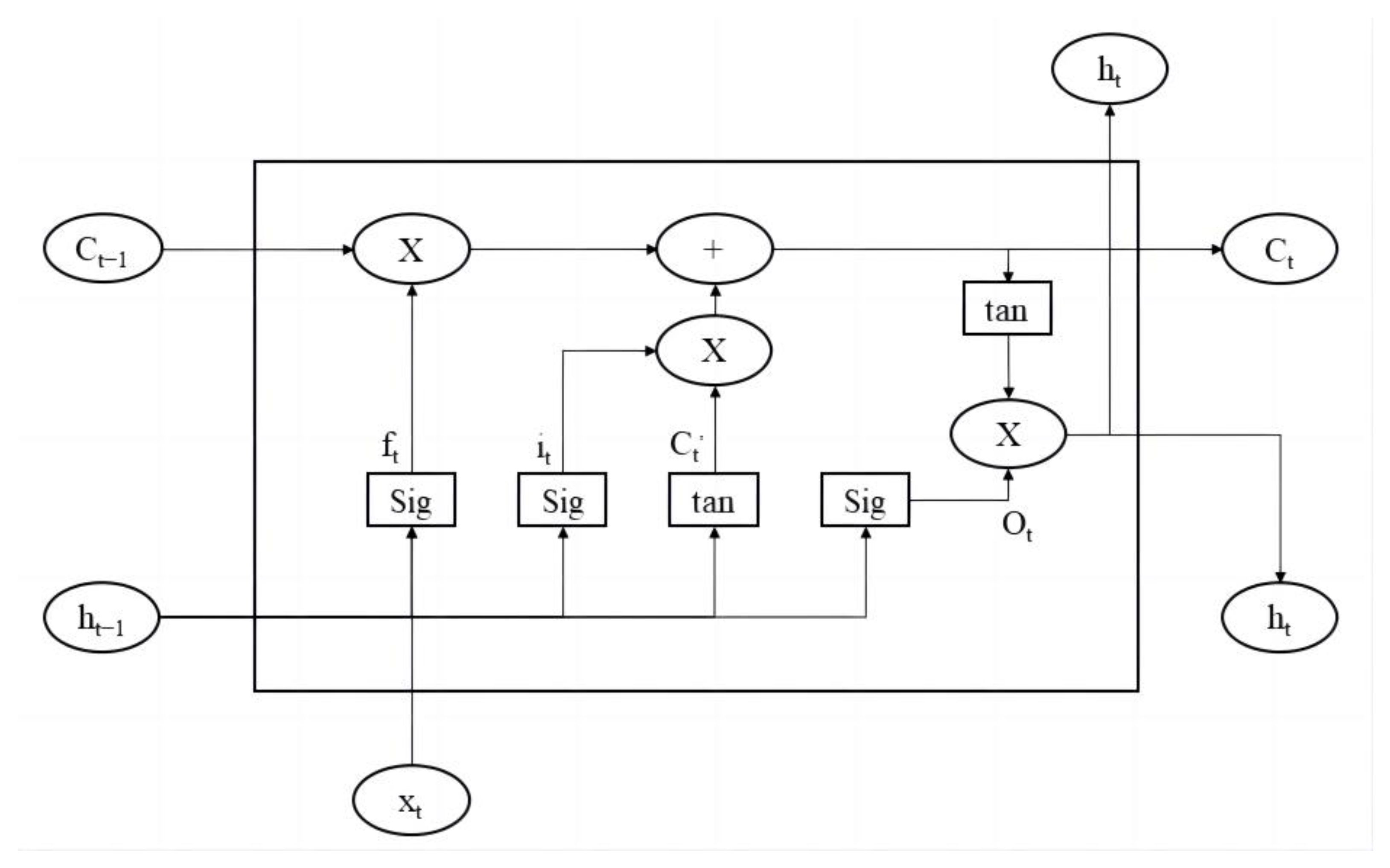
Figure 1 shows a schematic diagram of the LSTM neural network. The memory unit in the LSTM is controlled by the input gate it, the forgetting gate ft and the output gate O_t. ft and it control the Ct content. The input gate it determines the extent to which the input x_t enters the current memory state Ct. The oblivion gate ft controls the transfer relation between the cell state C_t−1 at the previous moment and the current state C_t. The output gate O_t controls the proportion of the current state Ct output to ht. The three types of gates within each cell of the LSTM are all determined by the Sigmoid activation function as to whether to activate or not, and the final output is determined by both the output gate and the cell state. They are calculated in turns.

$${\mathrm{i}}_{\mathrm{t}}=\mathsf{\sigma }\left({\mathrm{W}}_{\mathrm{i}}\left[{\mathrm{h}}_{\mathrm{t}-1},{\mathrm{x}}_{\mathrm{t}}\right]{+\mathrm{b}}_{\mathrm{i}}\right)$$

(1)

$${\mathrm{f}}_{\mathrm{t}}=\mathsf{\sigma }\left({\mathrm{W}}_{\mathrm{f}}\left[{\mathrm{h}}_{\mathrm{t}-1},{\mathrm{x}}_{\mathrm{t}}\right]{+\mathrm{b}}_{\mathrm{f}}\right)$$

(2)

$${\mathrm{C}}_{\mathrm{t}}{=\mathrm{f}}_{\mathrm{t}}{\mathrm{C}}_{\mathrm{t}-1}{+\mathrm{i}}_{\mathrm{t}}\tanh \left({\mathrm{W}}_{\mathrm{c}}\left[{\mathrm{h}}_{\mathrm{t}-1},{\mathrm{x}}_{\mathrm{t}}\right]{+\mathrm{b}}_{\mathrm{c}}\right)$$

(3)

$${\mathrm{O}}_{\mathrm{t}}=\mathsf{\sigma }\left({\mathrm{W}}_{\mathrm{o}}\left[{\mathrm{h}}_{\mathrm{t}-1},{\mathrm{x}}_{\mathrm{t}}\right]{+\mathrm{b}}_{\mathrm{o}}\right)$$

(4)

$${\mathrm{h}}_{\mathrm{t}}{=\mathrm{O}}_{\mathrm{t}}\tanh \left({\mathrm{C}}_{\mathrm{t}}\right)$$

(5)

where σ is the Sigmoid activation function, tanh for the activation function of C_t, C_t is the unit state vector, h_t is the state of the hidden layer, W is a matrix of weighting factors, and b is the bias vector of the input gate.

2.2. Overview of the XGBoost Model

XGBoost is an integrated learning framework based on the Boosting tree model with a second-order Taylor expansion of the loss function. Compared to the GBDT model, the training time is reduced, which in turn improves the efficiency of the solution, and the inclusion of a regular term reduces the complexity of the model and prevents over-fitting.

The core idea of the algorithm is to build new trees by continuously splitting features to fit the residuals between the last prediction and the actual value, and to sum up the results of all trees as the final prediction result. The integration model equation is,

$${\hat{\mathrm{y}}}_{\mathrm{i}}={\displaystyle \sum }_{\mathrm{k}=1}^{\mathrm{k}}{\mathrm{f}}_{\mathrm{k}}\left({\mathrm{x}}_{\mathrm{i}}\right),{\mathrm{f}}_{\mathrm{k}}\in \mathrm{F}$$

(6)

where f_k(x_i) is the kth decision tree, k is the serial number of the tree, x is the eigenvector, y for sample labels, F for the tree model, and ${\widehat{y}}_i$ is the predicted value. The objective function of the XGBoost algorithm is shown below.

$$\mathrm{L}={\displaystyle \sum }_{\mathrm{i}=1}^{\mathrm{n}}\mathrm{l}\left({\mathrm{y}}_{\mathrm{i}},{\hat{\mathrm{y}}}_{\mathrm{t}}\right)+{\displaystyle \sum }_{\mathrm{k}=1}^{\mathrm{k}}\mathsf{\Omega }\left({\mathrm{f}}_{\mathrm{k}}\right)$$

(7)

$$\mathsf{\Omega }\left({\mathrm{f}}_{\mathrm{k}}\right)=\mathsf{\gamma }T+\frac{1}{2}\mathsf{\lambda }{||w||}^2$$

(8)

where l is the loss function, i.e., the error between the predicted and true values, $\mathsf{\Omega }$ is the regularization function, T is the total number of leaf nodes in each tree, t is the weight of each leaf node of the tree, and $\mathsf{\gamma }$ and $\mathsf{\lambda }$ are hyperparameters.

Update the objective function with each iteration.

$${\mathrm{L}}^{\left(\mathrm{t}\right)}={\displaystyle \sum }_{\mathrm{i}=1}^{\mathrm{n}}\mathrm{l}\left({\mathrm{y}}_{\mathrm{i}},{\hat{\mathrm{y}}}^{\left(\mathrm{t}-1\right)}{+\mathrm{f}}_{\mathrm{t}}\left({\mathrm{x}}_{\mathrm{i}}\right)\right)+\mathsf{\Omega }\left({\mathrm{f}}_{\mathrm{t}}\right)$$

(9)

In order to optimize the objective function, a second order Taylor expansion is performed on the loss function part of the objective function.

$${\mathrm{L}}^{\mathrm{t}}={\displaystyle \sum }_{\mathrm{i}=1}^{\mathrm{n}}\mathrm{l}[{\mathrm{y}}_{\mathrm{i}},{\hat{\mathrm{y}}}_{\mathrm{i}}^{\left(\mathrm{t}-1\right)}{+\mathrm{g}}_{\mathrm{i}}{\mathrm{f}}_{\mathrm{t}}\left({\mathrm{x}}_{\mathrm{i}}\right){+\mathrm{h}}_{\mathrm{i}}{\mathrm{f}}_{\mathrm{t}}^2\left({\mathrm{x}}_{\mathrm{i}}\right)/2]+\mathsf{\gamma }\mathrm{T}+\frac{\mathsf{\lambda }}{2}{\displaystyle \sum }_{\mathrm{i}=1}^{\mathrm{T}}{\mathrm{w}}_{\mathrm{i}}^2$$

(10)

where g_i and h_i are univariate quadratic functions that are independent of each other.

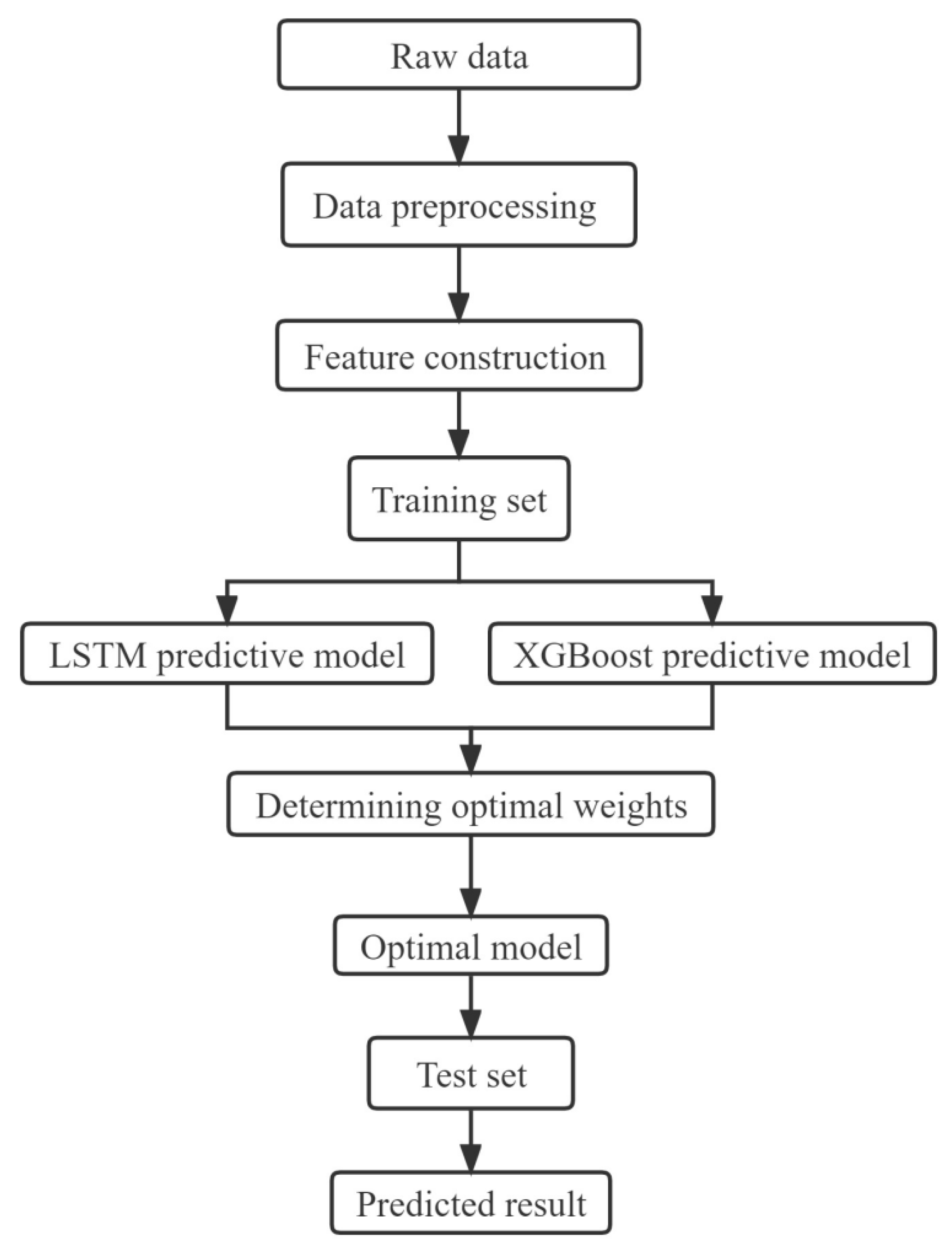
2.3. Combined LSTM-XGBoost Model Implementation Method

Traffic flow forecasting is a problem based on regression of continuous target variables, and commonly used models such as multiple regression models, GBDT, XGBoost and LSTM are effective in solving such problems. However, there are some differences in the process and principles of data processing between the different single models, and different prediction results are obtained. In order to combine the advantages of the different models, the LSTM neural network model and the XGBoost model are mixed in this paper. The overall forecasting model architecture is shown in Figure 2.

Since the neural network model and the tree model produce low correlation results, this paper uses a genetic algorithm to select the optimal weighting parameters. The method helps to improve prediction accuracy and the specific steps of the hybrid model algorithm are as follows.

(1)

Using the LSTM model to predict the data to acquire ${\widehat{y}}_i$.

(2)

Prediction of the data using the XGBoost model yields ${\widehat{y}}_j$.

(3)

Training of model weights α and β by means of equation $\widehat{y}=\mathsf{\alpha }{\widehat{y}}_i+\mathsf{\beta }{\widehat{y}}_j$ and genetic algorithms.

(4)

The weights obtained were assigned as single model weights in the mixed model and linearly summed to obtain $\widehat{y}$.

2.4. Example Analysis

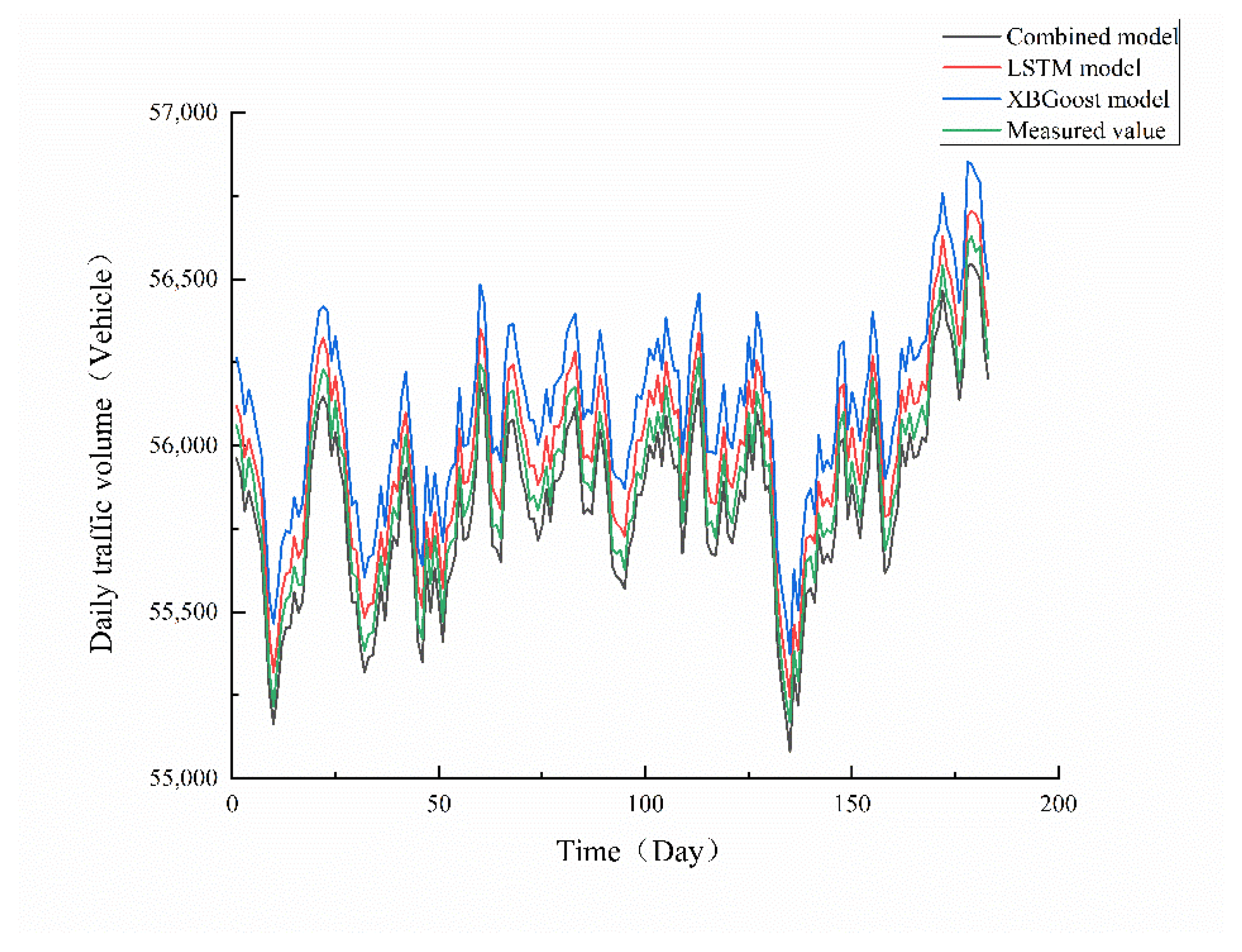
This paper uses historical traffic data provided by the bridge toll booth from 30 June 2011 to 30 June 2022 for the simulation analysis. The data are sampled at daily intervals and counted once a day. There are 4018 sets of data in the dataset. The first 126 months of data were selected as the training set and the last 6 months of data were chosen as the test set. The test results are shown in Figure 3.

The results of the calculations are shown in

Table 1. A comparison of MAE, MAPE and RMSE for different models.

Model	MAE/Vehicle	MAPE/%	RMSE/Vehicle
LSTM	88.1141	0.16	89.8220
XGBoost	116.5163	0.19	117.7853
Combined model	74.0163	0.13	75.7115

. The MAE, MAPE and RMSE values for the combined LSTM-XGBoost model were 074.0163, 0.13 and 75.7115, respectively. The model has a smaller error compared to the single model, indicating the highest prediction accuracy and better suitability for traffic flow forecasting on this bridge.

3. Finite Element Analysis Model

3.1. Background of the Study

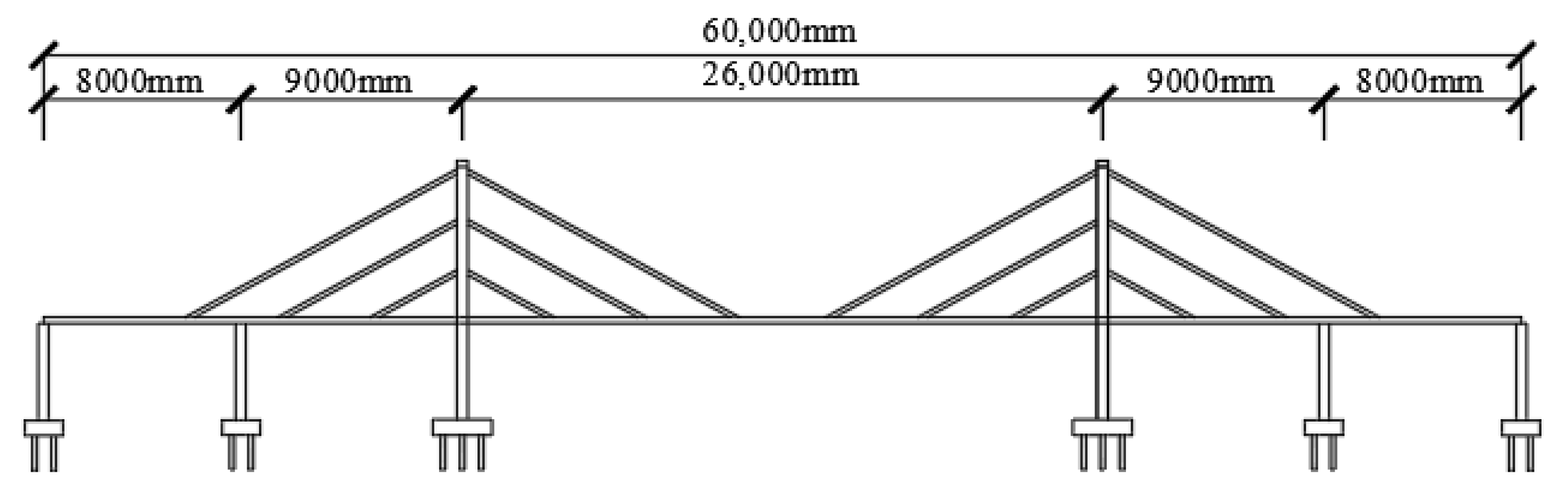
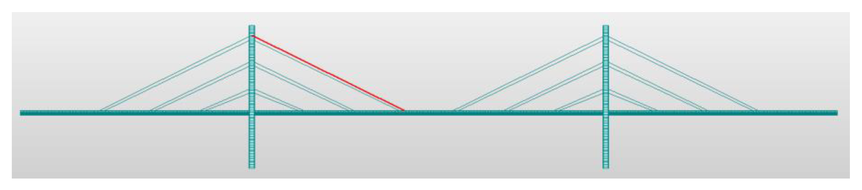
This cross-sea cable-stayed bridge is a double span detached double tower double rope surface steel box girder cable-stayed bridge, which adopts a five-span continuous semi-floating structural system with a main bridge span of (80 + 90 + 260 + 90 + 80 m). The main girder is a flat streamlined closed steel box girder with orthogonal anisotropic plate upper flanges. The diagonal cables are made of high strength parallel steel wire cables.

The towers are H-shaped transversely, and the columns are vertical upwards. The spacing between the towers is 30.5 m and the spacing between the towers is 20.6 m. The bottom elevation of the towers is 5 m and the top elevation of the towers is 105 m, with the lower towers below the top edge of the crossbeam being 39 m high and the upper towers above the top edge of the crossbeam being 66 m high.

The cables are made of 96 parallel steel cables. The width of the steel box sorghum is 24 m including the wind spout, 19.9 m without the wind spout, and 3.5 m high at the center line of the width. The design seismic basic intensity VI degrees, design load rating for city-A and highway-I are detailed. Figure 4 shows the general layout of the main bridge.

3.2. Building a Finite Element Model

In order to carry out a time course analysis of the bridge, a finite element analysis model of the bridge structure is required in this section. The bridge consists of two symmetrical left and right spans, so for the sake of simplicity, only half of the bridge structure is built in this paper. The calculation model is based on a combined unit model consisting of a truss unit and a beam unit. Beam units are used for the box girders and towers, and truss units for the diagonal cables. There are a total of 1123 nodes and 1116 units in the bridge model, of which 1068 are girder units and 48 are truss units. The model uses the horizontal bridge direction as the X-axis, the vertical bridge direction as the Y-axis and the vertical direction as the Z-axis, with X, Y and Z conforming to the right-hand rule. The unit of length in the model is taken as m and the unit of force is N. The finite element model diagram of the bridge structure is shown in Figure 5.

The initial material parameters for the bridge calculation model were designed as shown in the

Table 2. The table of initial design parameters for main materials.

Projects	Materials	Capacity	Modulus of Elasticity	Poisson Ratio
Cable tower	C50 Concrete	25 kN/m3	3.45 × 104 MPa	0.2
Main beam	Q345 steel	77 kN/m3	2.06 × 105 MPa	0.3
Crossbeam	C50 Concrete	25 kN/m3	3.45 × 104 MPa	0.2
Prestressed steel bundles	15–22 Steel strand	78.5 kN/m3	1.95 × 105 MPa	0.3
Inclined ropes	Steel wire	78.5 kN/m3	1.95 × 105 MPa	0.3

below.

Based on the actual forces applied to the bridge structure during operation, the following main sub loads were determined as shown in

Table 3. The bridge sub-load table.

Load	Remarks
Self-weight	Automatic software calculation
Phase II Loads	31 kN/m
Prestressing loads	Added by actual prestressing loads
Overall warming	Steel construction 31.2 °C Concrete 16.5 °C
Overall cooling	Steel construction 32 °C Concrete 18.2 °C
Wind loads	25 m/s
Crowd loads	2.5 kN/m2
Slanting cable forces	Add according to actual initial tension

.

The boundary conditions of the cable-stayed bridge were simulated according to the structural system constraint system with the constraints shown in

Table 4. The table of structural system constraints.

Binding Directions	Transition Pier	Auxiliary Pier	Cable Tower
Longitudinal orientation	Unbinding	Unbinding	Viscous dampers
Horizontal orientation	Binding	Viscous dampers	Binding
Vertical orientation	Binding	Binding	Binding

.

3.3. Time Course Analysis

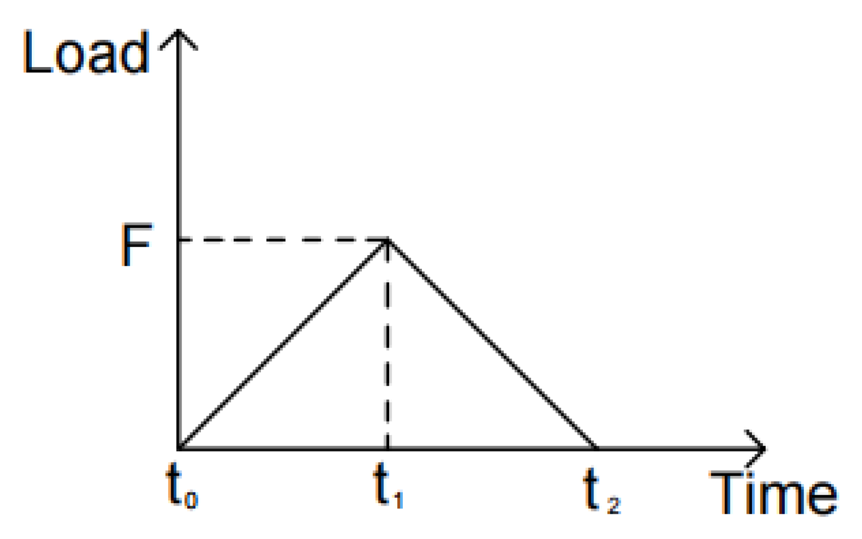
As the vehicle load acts on the node, it is a shock load that disappears instantly. This is approximated in Midas/Civil as a triangular load with a maximum value of F as shown in Figure 6. Where the time difference between time t₀–t₁ and t₁–t₂ is determined by the speed of the vehicle and the spacing between adjacent nodes. It is assumed that the effect of the force at node j when the time-varying load is applied to node i is zero. The effect of the force at node j when the time-varying load is applied at point j is 100%.

Vehicle loads are dynamic loads, i.e., loads that vary in size, direction or point of action with time. The displacement, internal forces, stresses and strains of a structure under dynamic loading are also constantly changing with time. One of the most important differences between dynamic and static loads is that dynamic problems take into account inertia forces due to the acceleration of the structure. The time course analysis is a method for calculating the corresponding structure under dynamic loads. Its essence is to obtain the response of the structure at each moment and the variation of the response as a function of time by taking the dynamic action.

4. Dynamic Simulation Analysis under Different Traffic Flow Loads

Considering the current traffic condition and the future traffic flow increasing continuously, the state of the main bridge under different traffic flow is simulated. The changes of the stresses in the main sections, the stresses in the diagonal cables, and the deflections in the span of the main girders are examined to provide a basis for the bridge management.

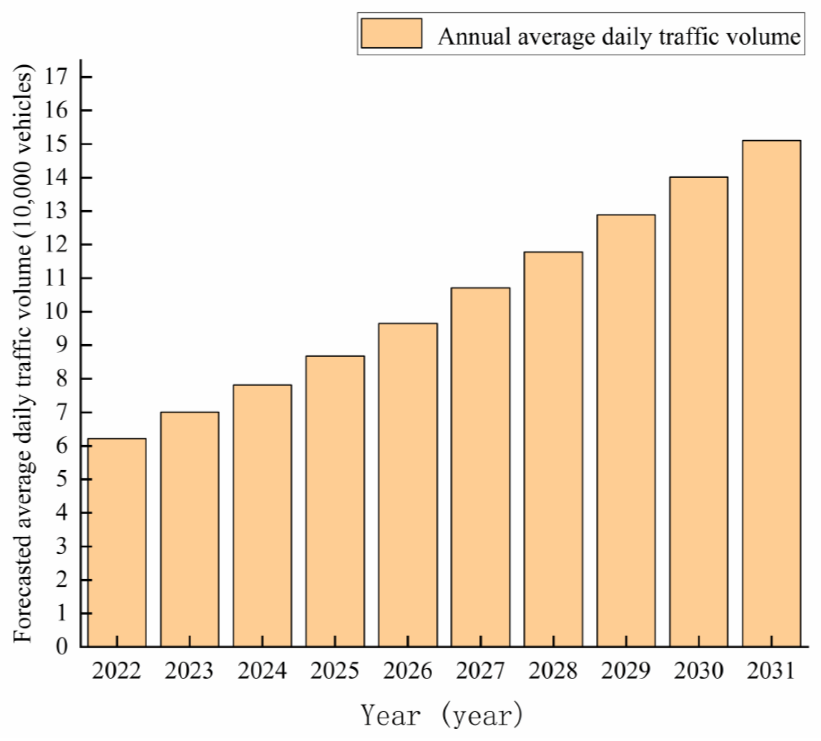
In this chapter, based on the traffic flow forecasting results of the combined LSTM-XGBoost model, 10 working conditions for simulating future traffic volumes are identified. The traffic volume prediction results of the bridge are shown in Figure 7.

The predicted traffic volume of 10 years was selected as the working condition. For the above 10 working conditions, because the bridge is a city highway bridge, the design speed is 80 km/h. The main vehicle is about a 3 t family car, considers the average single vehicle weight as 30 kN and has a simulated vehicle load in 24 h averages through the bridge.

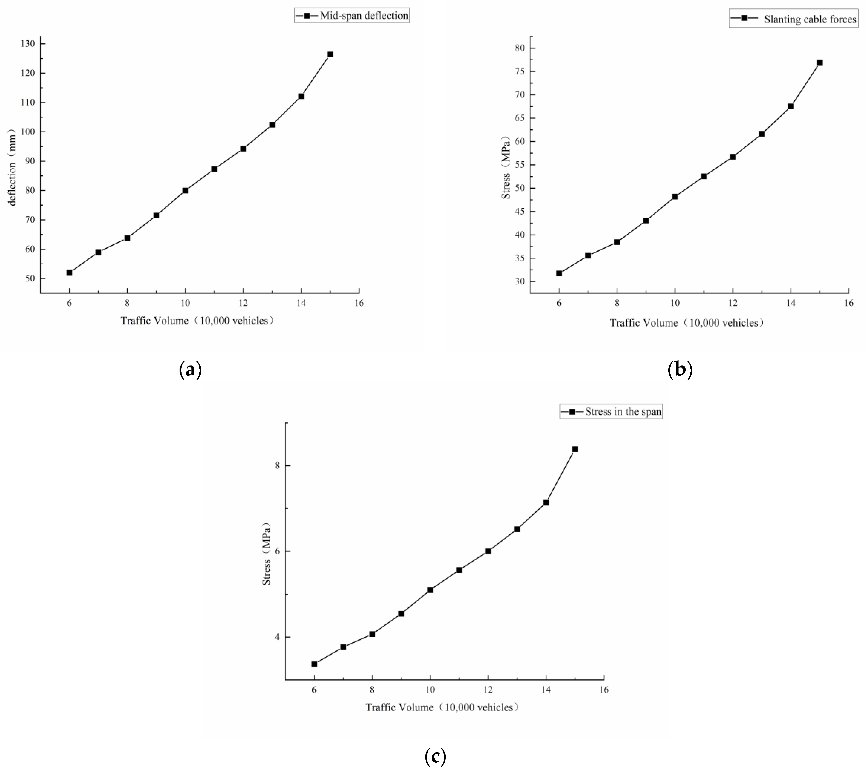
4.1. Influence of Different Traffic Volumes on Spanwise Deflection of the Main Beam

The variation of deflection at the mid-span of the main beam under different traffic flow conditions was calculated according to the time course analysis method, and the results are shown in Figure 8a.

It can be seen from Figure 8a that the deflection of the bridge main girder increases with the increase of traffic flow. When the traffic volume increases from 60,000 to 150,000 vehicles, the deflection increases from 51.97 mm to 126.36 mm, an increase of nearly 143%. From the span deflection alone, the change in traffic volume has a large effect on the span deflection. By fitting the calculated data to a polynomial, the relationship between the span deflection and traffic volume for this bridge can be derived as shown below: y = 0.0186x⁴ − 0.7348x³ + 10.771x² − 61.957x + 171.03.

4.2. Influence of Different Traffic Volumes on the Stress of the Diagonal Cable

According to the analysis of the cable force variation of the bridge, the cable No. 1133, which has the largest variation, was selected as the object of analysis. According to the above method, the force change of cable No. 1133 was calculated under different traffic flow conditions. Here, the 1133 cable position is shown in Figure 8. The calculation results are shown in Figure 9.

It can be seen from Figure 8b that the stress of the diagonal cable No. 1133, which has the largest change, increases gradually as the traffic flow increases. When the traffic volume increases from 60,000 to 150,000 vehicles, the stress of the diagonal cable increases from 31.73 MPa to 76.87 MPa, and the change of cable force is about 2.4 times of the original one. Considering the diagonal cable stress alone, the change in traffic volume has less effect on the diagonal cable stress. By fitting the data polynomially, the relationship between deflection and traffic volume in the span of the bridge can be derived as follows: y = 0.0144x⁴ − 0.5733x³ + 8.4552x² − 50.223x + 134.13.

4.3. Effect of Different Traffic Volumes on Stresses in the Span of the Main Beam

The changes of stresses in the main beam mid-span span under different traffic flow conditions were calculated according to the above method, and the results are shown in Figure 8c.

It can be seen from Figure 8c that the stresses at the mid-span span gradually become larger as the traffic volume increases. As the traffic volume increases from 60,000 to 150,000 vehicles, the stress at the midspan span increases by 5.017 MPa. In terms of the span stress in the main girder, the change in traffic volume has less effect on the span stress in the midspan girder unit. A polynomial fit of the data gives the following relationship between the span-middle girder unit stress and traffic volume: y = 0.0022x⁴ − 0.089x³ + 1.3015x² − 7.8378x + 19.906.

4.4. Bridge Traffic Management Analysis

4.4.1. Passable Traffic Volume

According to Article 7.2.5 of the Design Specification for Highway Cable-stayed Bridges (JTG/T 3365-01-2020), the fitting formula is used for calculation. When the traffic volume increased to 230,000 vehicles, the deflection at the middle span of the bridge increased to 708 mm, and the cable-stayed stress and the stress in the span reached 506.17 MPa and 60.9 MPa, respectively. The results of the fitted data were basically the same as those calculated by the finite element software. This result shows that the fitting formula has high accuracy. The result has exceeded the limit value of the span deflection of this bridge. Considering the deflection, the limit traffic flow of the bridge can be estimated to be around 220,000 vehicles. According to the combined LSTM-XGBoost model, the maximum traffic volume is calculated to occur in 2038. Therefore, the bridge management should monitor the traffic volume statistically in time to avoid exceeding the limit traffic volume of the bridge.

4.4.2. Vehicle Travel Speed

According to the literature [24], the impact coefficient is minimized when the vehicle is driven at a constant speed. The impact coefficient at uniform acceleration driving is greater than uniform speed driving. The impact coefficient increases significantly when braking in the middle of the span, and the shorter the braking time, the larger the impact coefficient. Therefore, it is necessary to ensure that the vehicle passes the bridge at a constant speed without braking in order to minimize the impact coefficient. Therefore, for the bridge management, we should advocate the vehicle to pass at a constant speed of 80 km/h and avoid braking in the middle of the span.

5. Conclusions

This paper counts and processes traffic data for the bridge for the past ten years. A combined LSTM-XGBoost model was used to predict the traffic volume of the bridge for the next ten years. Based on the traffic predicted by the combined LSTM-XGBoost model, a simulation of changes in span section stresses, cable stresses and span deflections of main girders on the main bridge under predicted traffic volumes were established by means of finite element software. The following conclusions were drawn.

(1)

This paper is based on a combined LSTM-XGBoost model for traffic volume prediction. Comparing the combined LSTM-XGBoost model with a single model for prediction. The MAE, MAPE and RMSE values for the combined model were only 074.0163, 0.13 and 75.7115. The results show that the combined LSTM-XGBoost model has higher prediction accuracy than the single model.

(2)

In this paper, 10 traffic load conditions are simulated by finite element software under the combined LSTM-XGBoost model prediction. The variation of the stress state of the main beam, the stress in the diagonal cable and the deflection in the span were analyzed. The simulation data were fitted and analyzed to obtain the final fitted curves of the three with the predicted traffic volumes.

(3)

According to the results of the calculations, the limit traffic volume of the bridge is approximately 220,000 vehicles. According to the combined LSTM-XGBoost model, this maximum can be predicted to occur in 2038. If vehicles maintain a constant speed of 80 km/h when crossing the bridge, the structural condition of the bridge will be minimally affected.

References

- Liu, S.F.; Tao, L.Y.; Xie, N.M. On the New Model System and Framework of Grey System Theory. J. Grey Syst. 2016, 28, 1–15. [Google Scholar]
- Deifm, M.A.; Solyan, A.A.A.; Hammam, R.E. ARIMA Model Estimation Based on Genetic Algorithm for COVID-19 Mortality Rates. Int. J. Inf. Technol. Decis. Mak. 2022, 20, 1775–1789. [Google Scholar] [CrossRef]
- Zhang, J.; Zheng, Y.; Qi, D. Deep Spatio-Temporal Residual Networks for Citywide Crowd Flows Prediction; American Association for Artificial Intelligence: San Francisco, CA, USA, 2017. [Google Scholar]
- Luo, X.; Li, D.; Zhang, S. Traffic Flow Prediction during the Holidays Based on DFT and SVR. J. Sens. 2019, 2019, 6461450. [Google Scholar] [CrossRef] [Green Version]
- Jiao, P.P.; An, Y.; Bai, Z.X.; Lin, K. Research on short-time traffic flow prediction based on XGBoost. J. Chongqing Jiaotong Univ. (Nat. Sci. Ed.) 2022, 41, 17–23. [Google Scholar]
- Li, B.; Ming, Y.; Hao, Y.H.; Chen, S.S.; Wang, K.D. An analytical model for regulable potential of industrial large users based on fused FCN-TCN-LSTM. Power Autom. Equip. 2022, 1–16. [Google Scholar] [CrossRef]
- Zhao, X.Q.; Tuo, B.B.; Hui, Y.Y.; Jiang, H.M. Intermittent process quality prediction based on ISTA-LSTM model. Control Decis. Mak. 2022, 1–12. [Google Scholar] [CrossRef]
- Li, R.C.; Xiao, R.B. Optimized LSTM network based on improved wolf pack algorithm for public opinion evolution prediction. Complex Syst. Complex. Sci. 2022, 1–13. Available online: http://kns.cnki.net/kcms/detail/37.1402.n.20221009.1057.002.html (accessed on 1 October 2022).
- Yan, P.C.; Zhang, X.F.; Shang, S.X.; Zhang, C.Y. LIF combined with LSTM neural network for water source identification in mines. Spectrosc. Spectr. Anal. 2022, 42, 3091–3096. [Google Scholar]
- Tang, D.Q.; Zhu, W.; Hou, L.C. Ultra-short-term photovoltaic power prediction based on CNN-LSTM-XGBoost model. Power Technol. 2022, 46, 1048–1052. [Google Scholar]
- Wang, J.J.; Bi, L.; Zhang, K.; Sun, P.X.; Ma, X.D. Short-term photovoltaic power generation forecasting based on multi-feature fusion and XGBoost-LightGBM-ConvLSTM. J. Sol. Energy 2022, 1–7. [Google Scholar] [CrossRef]
- Tan, H.W.; Yang, Q.L.; Xing, J.C.; Huang, K.F.; Zhao, S.; Hu, H.Y. Power prediction of photovoltaic power generation based on combined XGBoost-LSTM model. J. Sol. Energy 2022, 43, 75–81. [Google Scholar]
- Dai, Y.M.; Zhou, Q. A combined power load forecasting method based on improved Bi-LSTM and XGBoost. J. Shanghai Univ. Technol. 2022, 44, 138–147. [Google Scholar]
- Zhou, L.T.; Deng, S.Y.; Liu, Z.K.; Gong, Y.Z. A prediction method for concrete dam deformation analysis based on SSA-LSTM-GF. J. Riverhead Univ. (Nat. Sci. Ed.) 2022, 1–17. Available online: http://kns.cnki.net/kcms/detail/32.1117.TV.20221009.0834.002.html (accessed on 1 October 2022).
- Zhan, M.Q.; Chen, B.; Liu, T.H.; Wang, F.S. Research on concrete dam deformation prediction based on variable weight combination prediction model. Hydropower Energy Sci. 2022, 40, 115–119. [Google Scholar]
- Yuan, W.Z.; Huang, H.Y.; Zhang, J.P.; Chen, B.C. Reliability study of existing bridges based on actual operational vehicle load effects. Vib. Shock. 2019, 38, 239–244. [Google Scholar]
- Yin, Z.X.; Li, H.S.; Li, H.M. Effects of overloaded vehicle action on steel truss girder suspension bridges. J. Liaoning Univ. Eng. Technol. (Nat. Sci. Ed.) 2016, 35, 618–623. [Google Scholar]
- He, Y.K. Design and Implementation of Automated Collection and Monitoring System for Health Monitoring of Cable-Stayed Bridges. Master’s Thesis, Chongqing Jiaotong University, Chongqing, China, 2016. [Google Scholar]
- Ma, N.X.; Xu, C.C.; Zhu, C.H.; Fu, W.B. Safety analysis of Jinan Yellow River Bridge on the Qingyin Line based on bridge health monitoring. Highway 2021, 66, 121–129. [Google Scholar]
- Wu, T. Analysis of the Impact of Vehicle Overloading on the Structure and Service Life of Bridges. Master’s Thesis, Shijiazhuang University of Railways, Shijiazhuang, China, 2019. [Google Scholar]
- Liu, Z.X.; Ai, Q.H.; Ruan, X.X.; Liu, Z.J. Analysis of dynamic response of high pier and large span bridges under multi-point multidimensional random earthquake. Eng. Seism. Reinf. Modif. 2022, 44, 52–59. [Google Scholar]
- Gu, Y.; Jin, B.H. Time analysis of dynamic response of high and low tower cable-stayed bridges under the action of moving vehicle loads. China Foreign Highw. 2018, 38, 190–194. [Google Scholar]
- Zhang, Y.Q. Static Dynamic Research on Short Tower Cable-Stayed Bridges for Large Span High-Speed Railways. Master’s Thesis, Southwest Jiaotong University, Chengdu, China, 2017. [Google Scholar]
- Chen, L.Q.; Chen, J.J. Research on traffic control measures for heavy vehicles passing on existing bridges. China Foreign Highw. 2018, 38, 153–157. [Google Scholar]
- Zhang, Y.B.; Sun, L.W. Structural simulation analysis of short tower cable-stayed bridge during operation. Railw. Archit. 2014, 7, 1–3. [Google Scholar]
- Yu, C.H.; Xia, B. Analysis of the dynamic response of a highway continuous girder bridge under the action of different vehicle speeds. Highway 2022, 67, 151–154. [Google Scholar]
- Ruan, X.; Zhou, J.; Caprani, C. Safety assessment of the anti-sliding between the main cable and middle saddle of a three-pylon suspension bridge considering traffic load modeling. J. Bridge Eng. 2016, 21, 4–16. [Google Scholar] [CrossRef]
- Zhu, J.; Wang, Y.W.; Li, Y.L.; Zheng, K.F.; Heng, J.L. Scour effect of cross-sea bridge under operation load and earthquake. J. Cent. S. Univ. 2022, 29, 2719–2742. [Google Scholar] [CrossRef]
- Xie, Y.C.; Gao, J.; Liu, C.L.; Liu, D. Influence of Moving Load on Dynamic Response of Bridge: A Case study of cracked prestressed concrete simple supported beams. Earthq. Disaster Prev. Technol. 2020, 15, 510–518. [Google Scholar]
- Ji, J.Y.; Wang, R.H.; Ma, N.J.; Yu, X.B.; Chen, M. Beam combination structure under moving load transient response analysis. J. Eng. Sci. Technol. 2022, 3, 192–200. [Google Scholar]
- Li, H.Q. Thoughts on Bridge Safety Operation Management. J. Highw. 2022, 67, 426–429. [Google Scholar]