CFD Study on the Influence of Exostructure Elements on the Resistance of a Submarine

Abstract

Submersible vessels designed to operate at low speeds are often designed with an intricate exostructure, as well as other elements that are located outside of the main pressure hull. Exostructure elements are often of cylindrical or rectangular shape, positioned perpendicularly to the flow direction. For this reason, their resistance coefficient is relatively large compared to the pressure hull or appendages of a classical submarine. In some cases, the exostructure can significantly increase the wetted surface of the vessel and dominate its resistance. This paper presents a study on how different exostructure elements impact the overall resistance of a submarine relative to the resistance of the cylindrical, smooth, pressure hull. Additionally, the effect of depth is also considered. The study is conducted using the RANS-based CFD method. The subject of the study is a 25 m long tourist submarine designed for depths up to 40 m and a speed of up to 3 knots.

1. Introduction

The design of low-speed submersible vessels typically does not consider hydrodynamic resistance as one of the important design constraints. For this reason, these vessels often have intricate geometries, often unfavourable from the hydrodynamic resistance point of view. Furthermore, the geometry of various types of submarines is highly varying, depending on the purpose of the vessel and size. Thus, typical methods of approximating its hydrodynamic resistance are not available since there is little data on similar vessels, and since the geometry is not comparable to other shapes found in the field of naval architecture, such as ships or submarines. Calculating the resistance of these objects requires model-scale experiments or numerical simulations. These results are being published more frequently, increasing the overall level of knowledge on the topic.

The topic has attracted a number of researchers who have published their findings of specific projects or purely scientific investigations. Huifeng et al. [1] conducted CFD simulations of a towed manned submersible, calculating the resistance coefficient to be 0.82. Jiang et al. [2] presented a CFD study of the hydrodynamic resistance of an autonomous remotely operated submersible for forward motion and descent. Wei et al. [3] used the response surface method to optimise the hydrodynamic resistance of a submersible, where they varied the length of the stern, length of the bow, and aspect ratio of the rudder, among others. Kotb et al. [4] conducted an investigation on the drag of an 18 m long tourist submersible, separately calculating the hydrodynamic resistance for various parts of the submersible’s geometry. Phillips et al. [5] used CFD to investigate and compare hydrodynamic resistance of three different types of submersible hull design. Additionally, they studied the effect of a submersible’s bow shape on overall resistance, finding that an elliptical bow with a higher length-to-diameter ratio reduces resistance. Khan et al. [6] showed a study of how different pressure body shapes influence hydrodynamic resistance. They tested four different geometries, and concluded that a conic shape is most favourable. Karim et al. [7] studied the performance of the k-$\omega$ SST turbulence model for estimating submersible resistance in a 2D CFD investigation, also comparing different grids. Chen et al. [8] studied the effect of sailing depth on the resistance coefficients of the SUBOFF using a RANS approach.

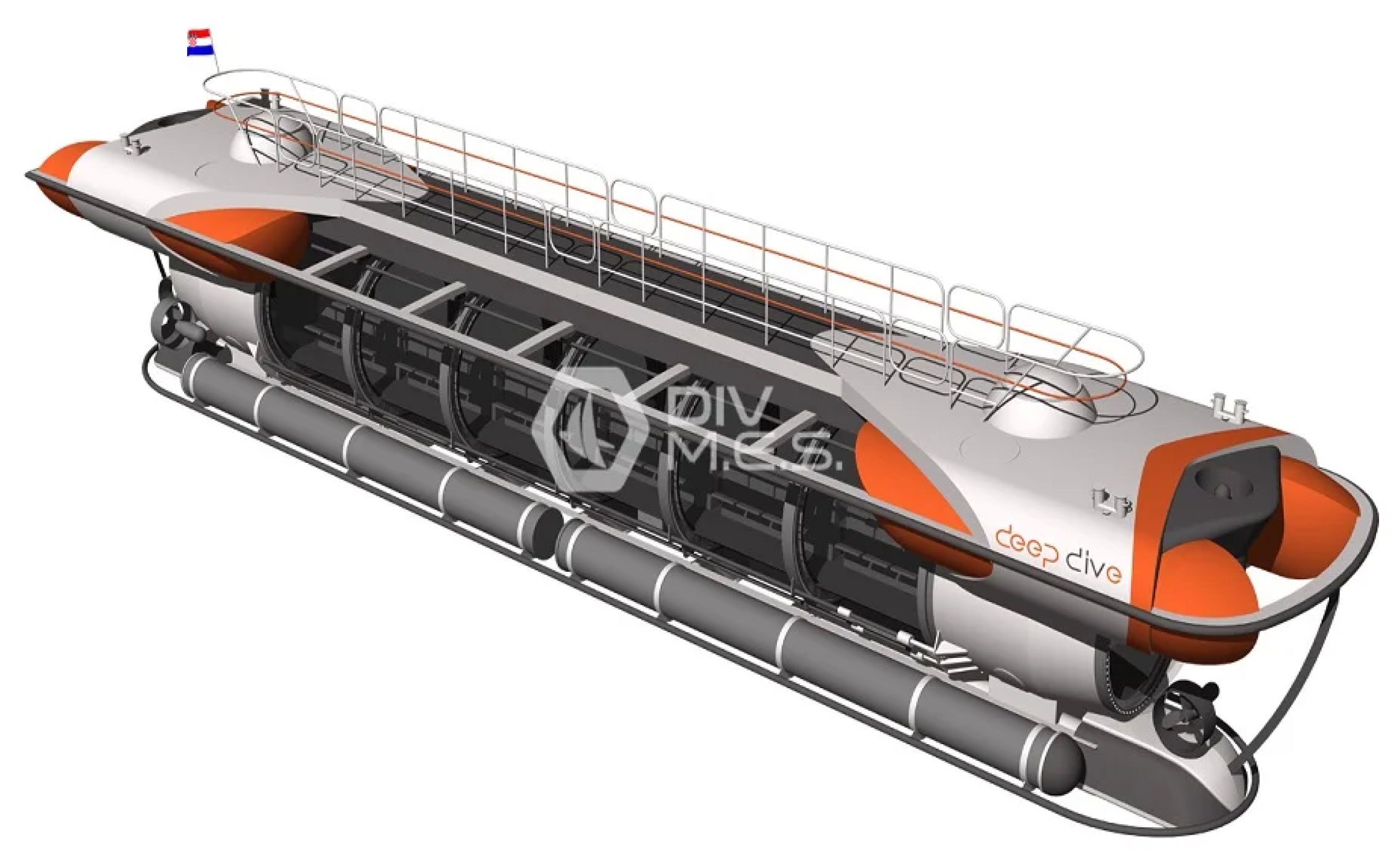
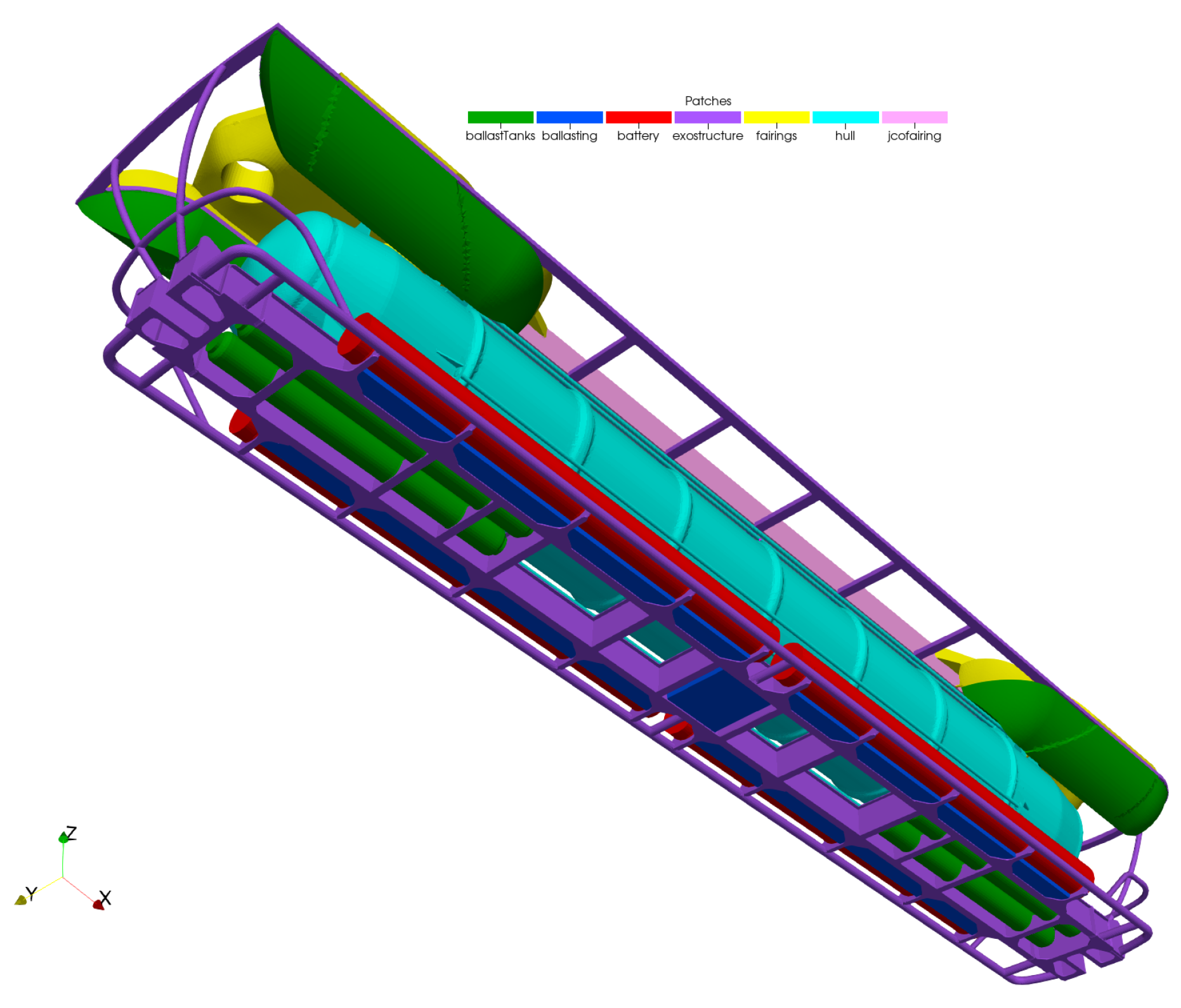
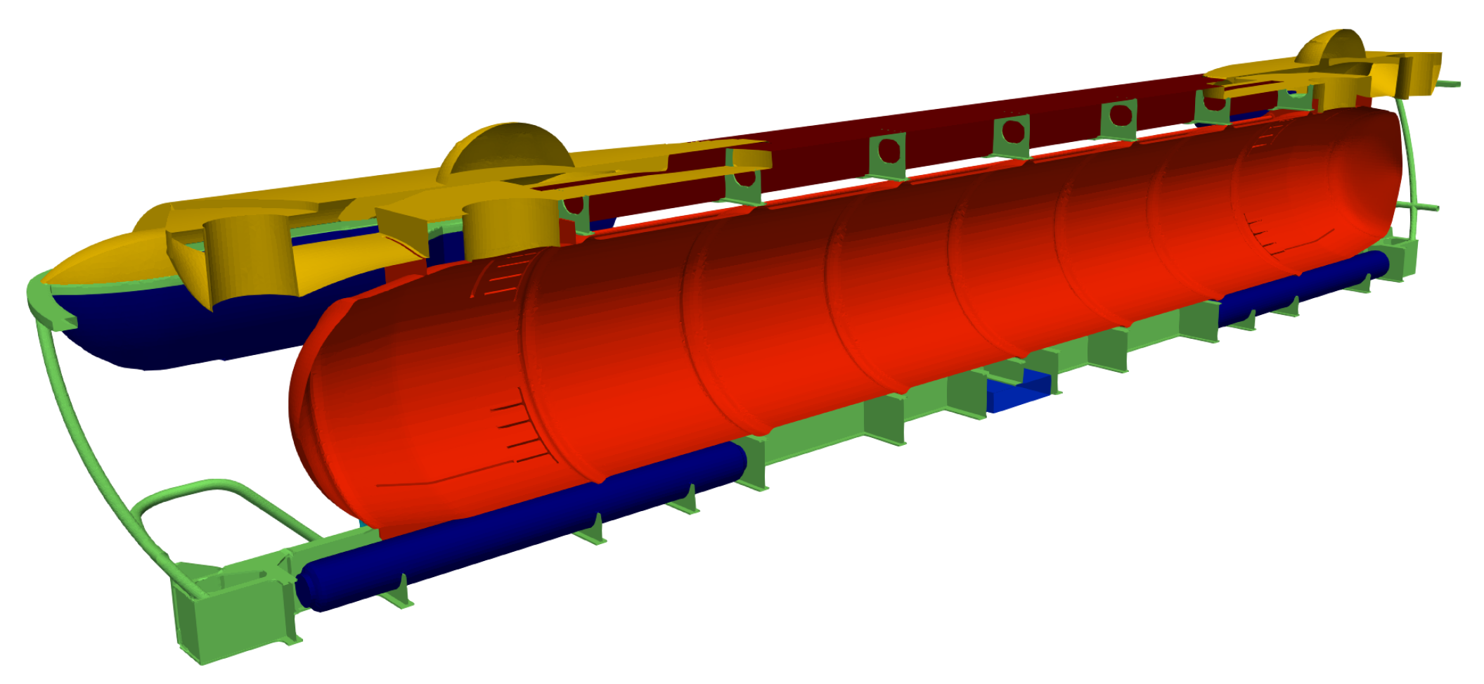
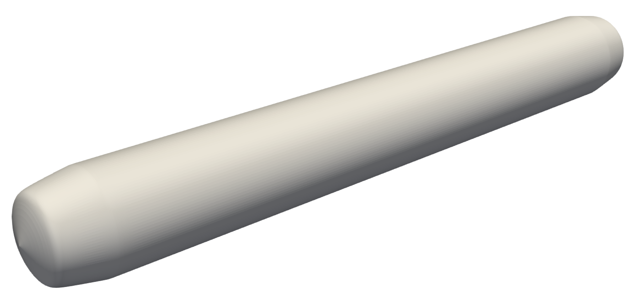
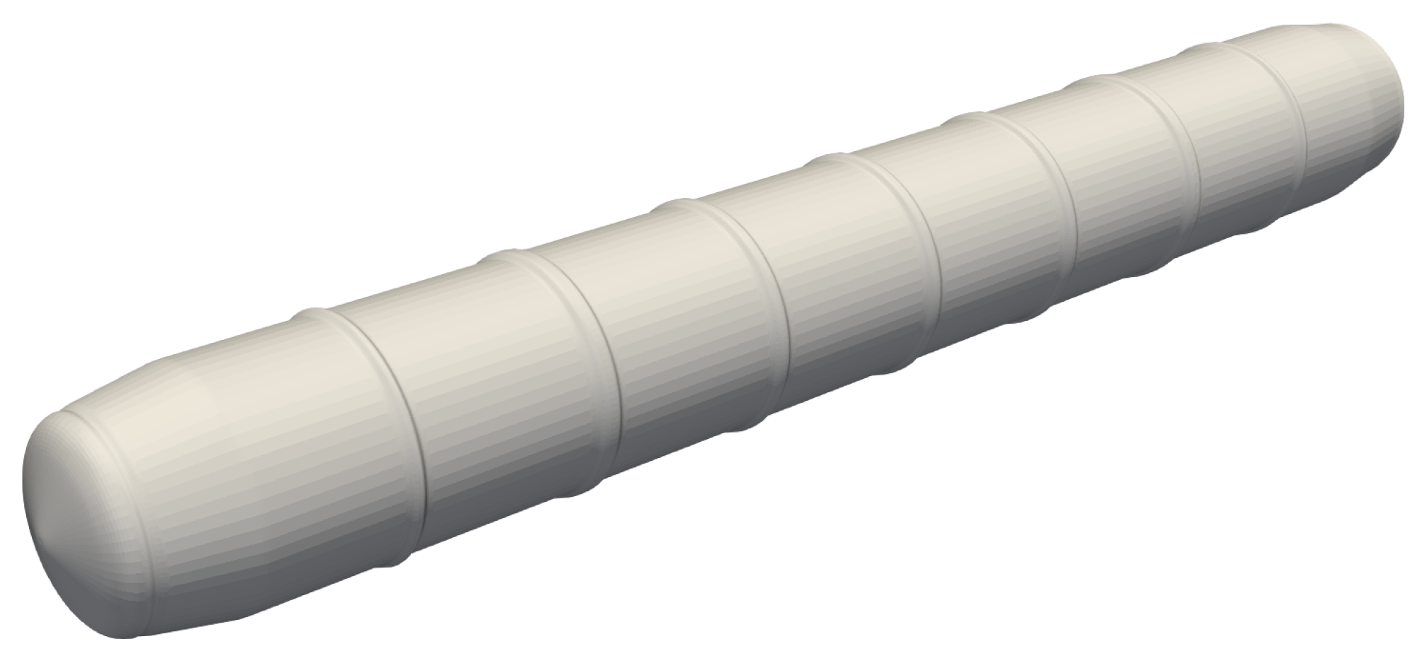
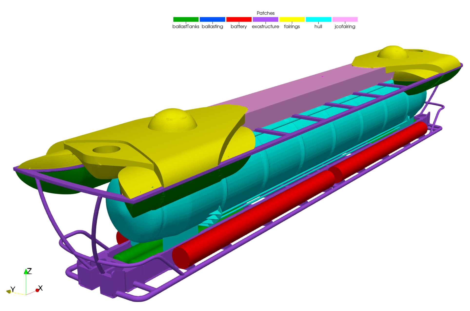
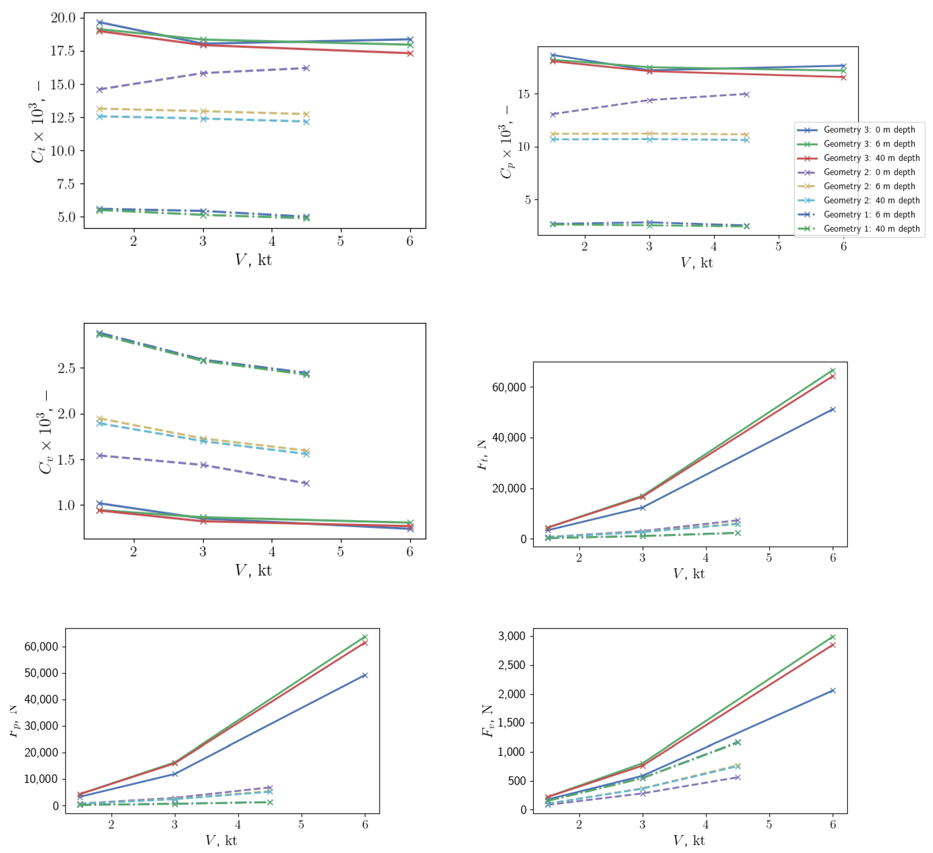
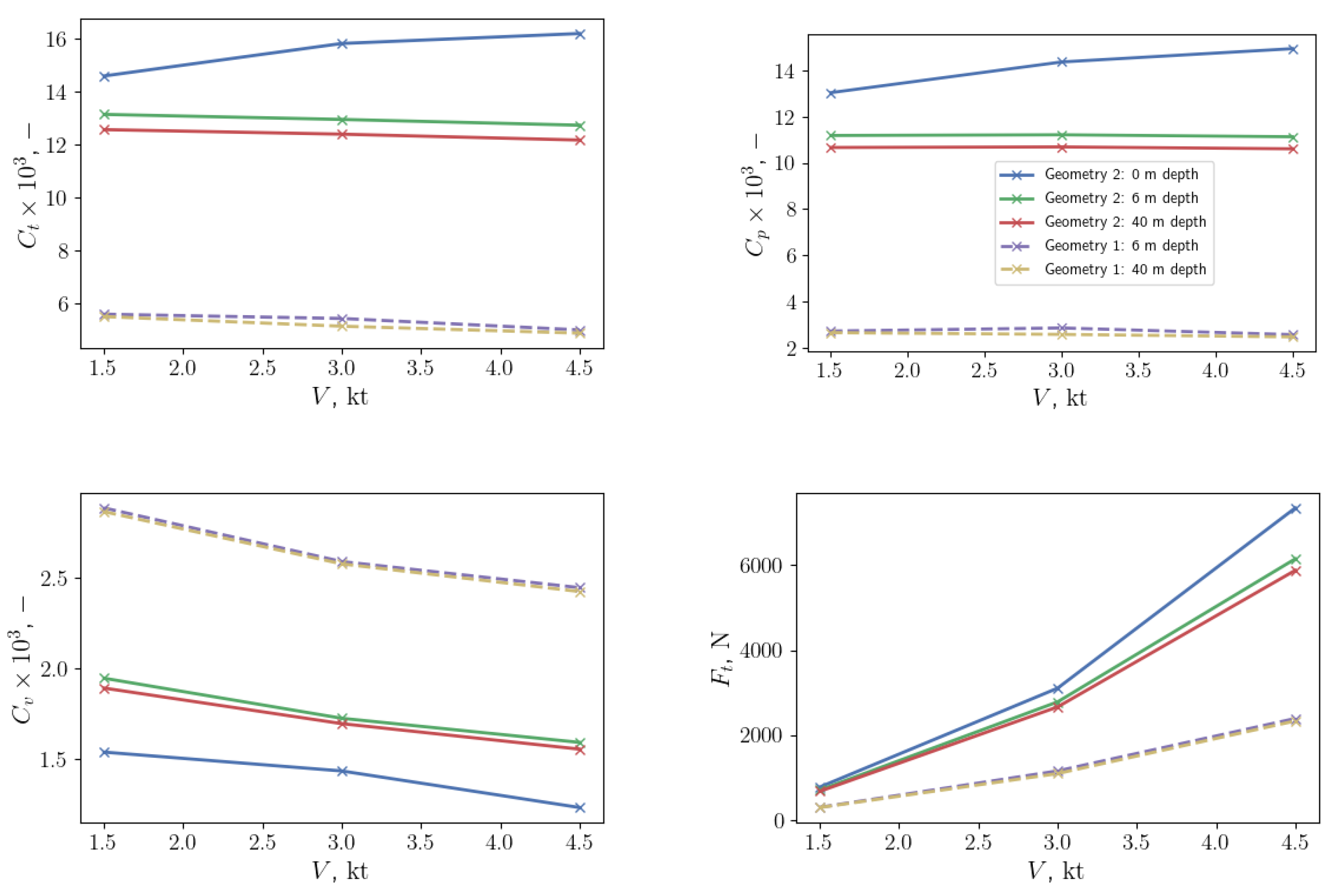
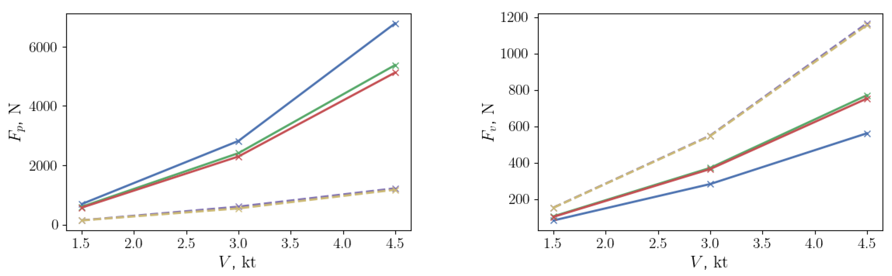
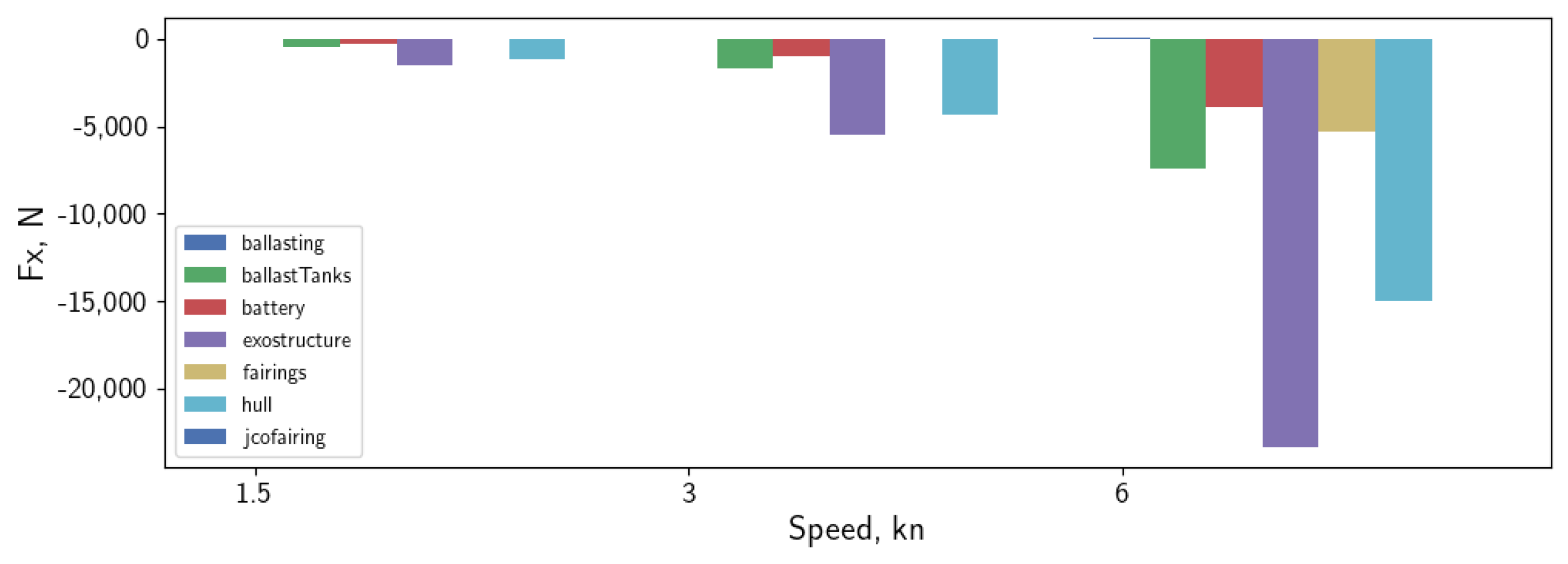
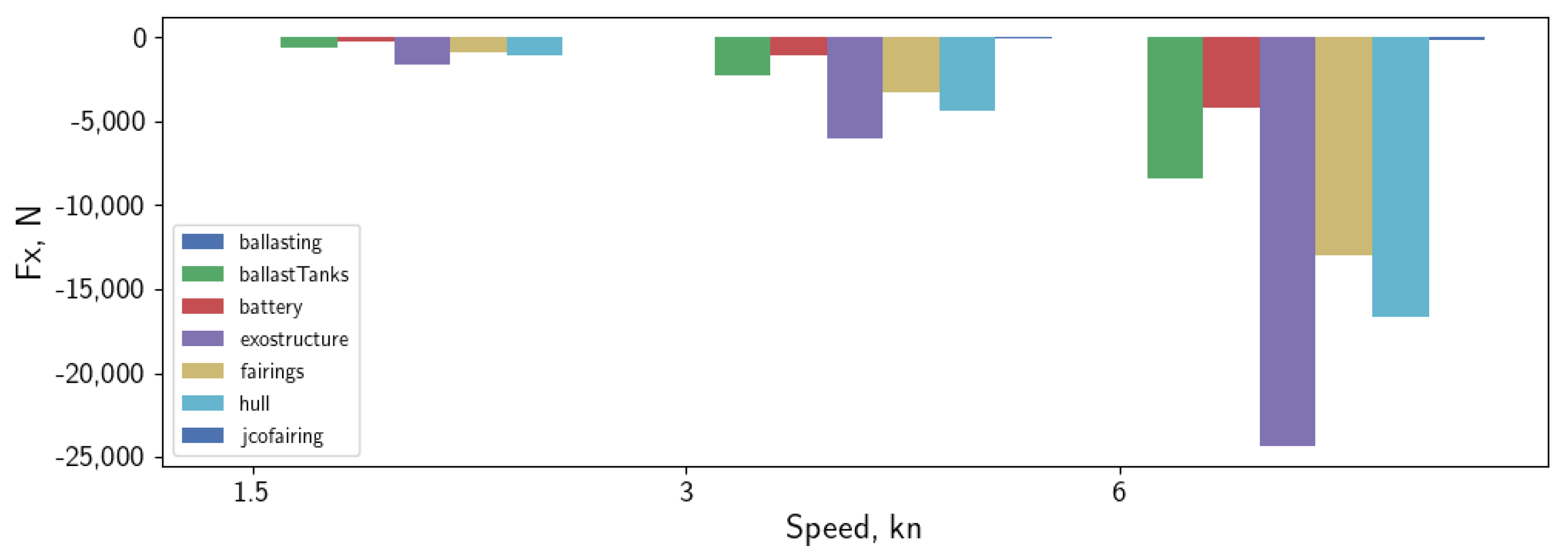
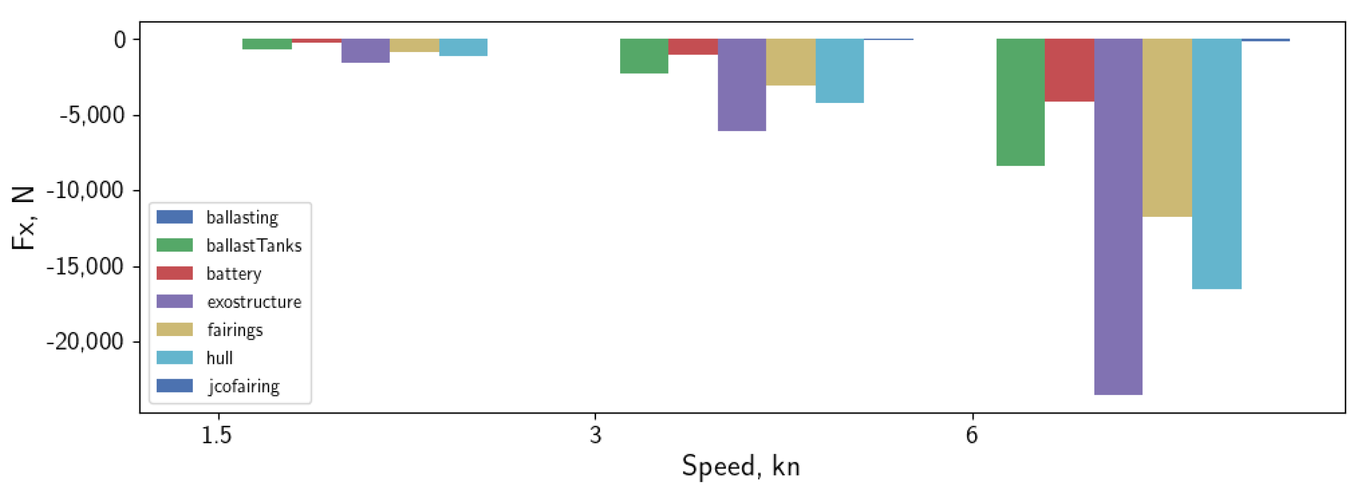
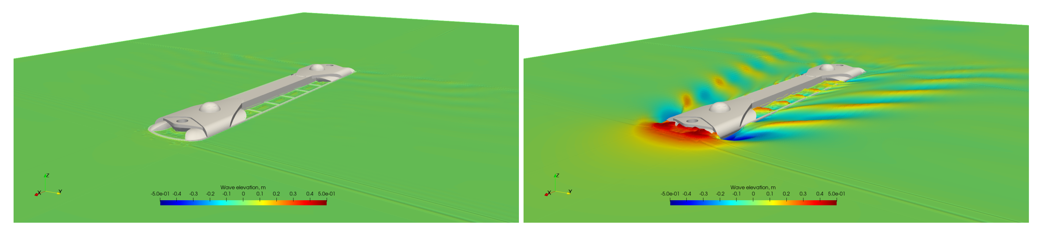
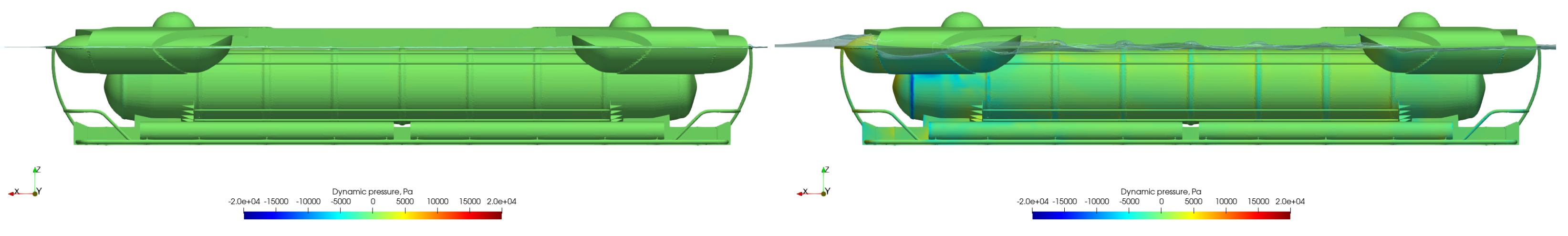
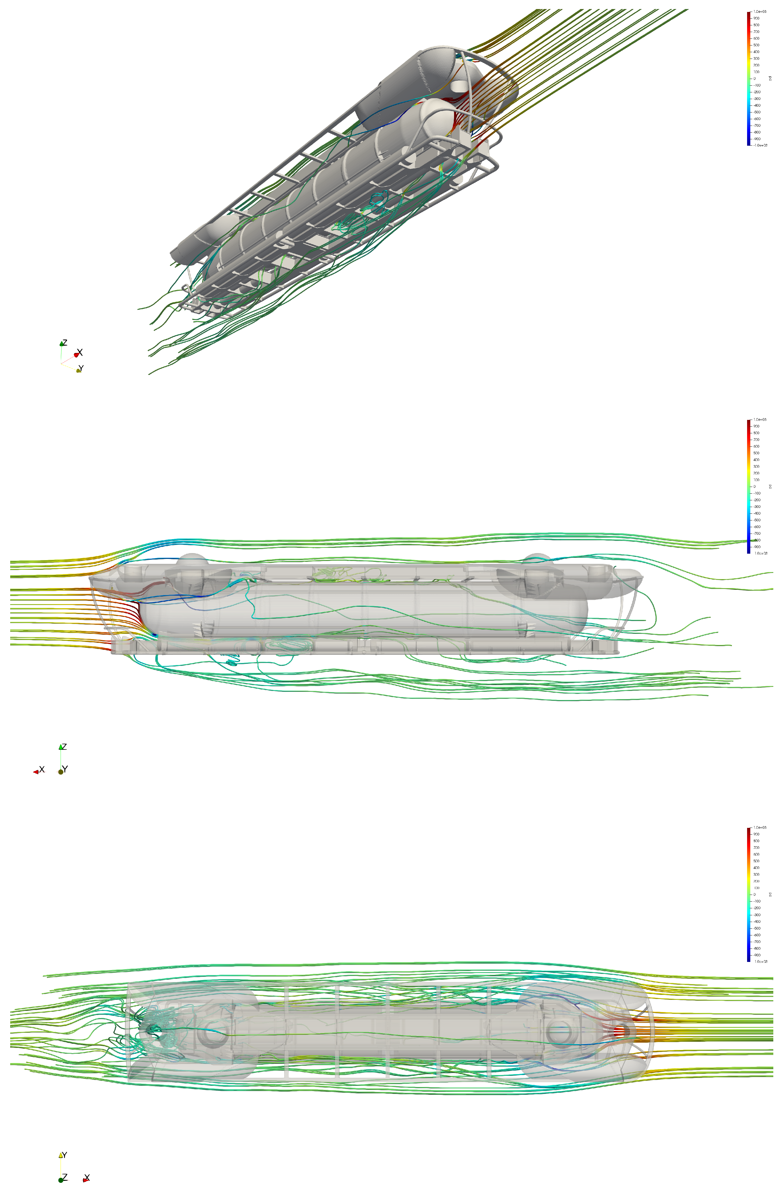
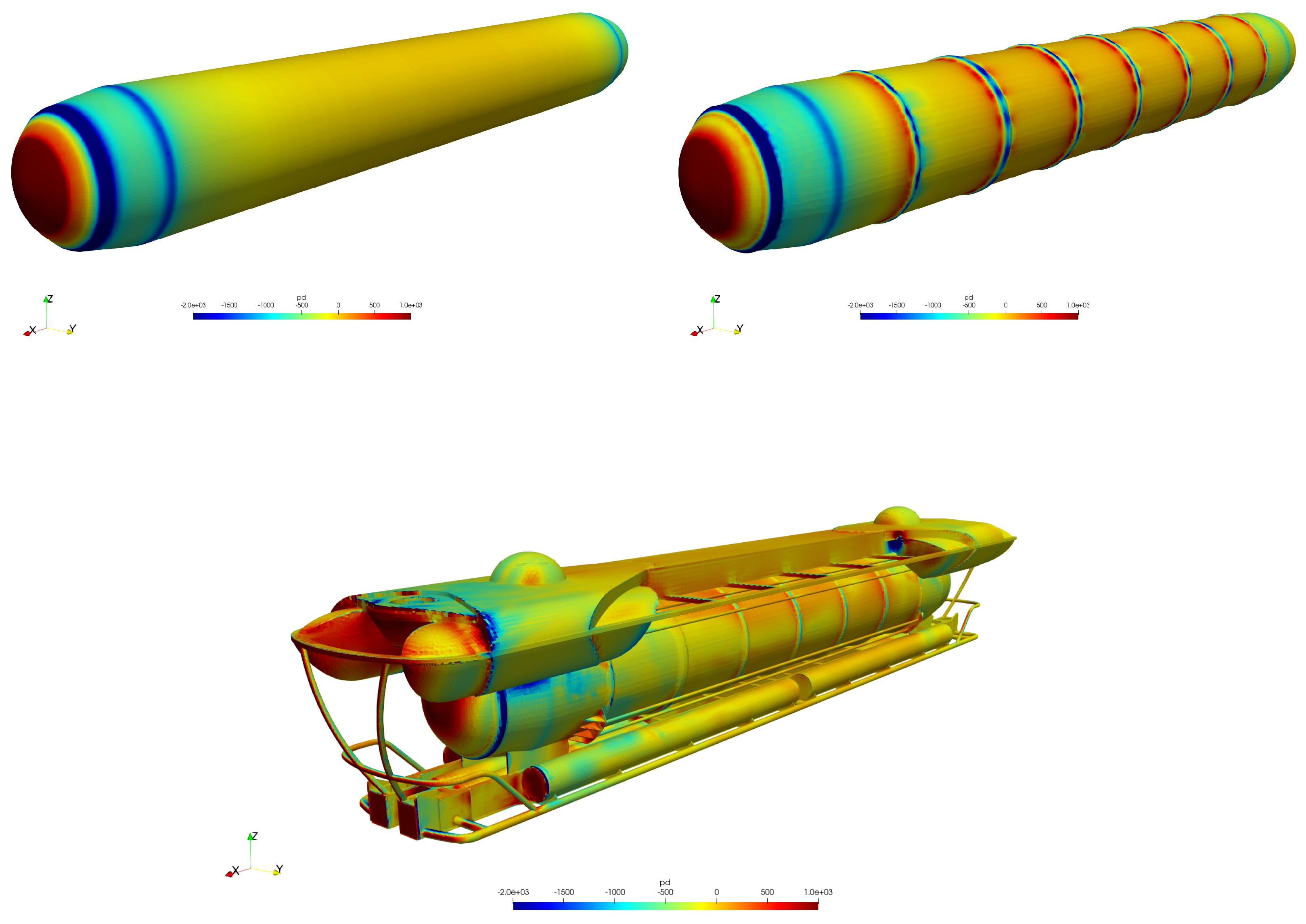
In this paper, an investigation of hydrodynamic resistance is conducted for a 25 m tourist submarine designed for depths up to 40 m and speeds up to 3 knots. More details about the structural design of this innovative underwater vehicle can be found in [9]. The main purpose of the study is to evaluate the total hydrodynamic resistance of the submarine and its contribution to the resistance of different hull elements. Additionally, the influence of structural elements orthogonally exposed to the flow to the overall resistance is studied. The effect of the free surface on the resistance is considered and analysed. The main goal of the present study is to gain a better understanding of how structural element placement (relative to flow) influences the resistance of the submarine, and how the total resistance behaves compared to conventional submarines. Three different geometry configurations are considered with different amounts of geometrical elements present outside the cylindrical pressure hull: smooth cylindrical pressure hull, pressure hull with orthogonal ring protrusions, and finally, the full geometry of the submarine, including the pressure hull with rings and other external elements. Resistance coefficients for different geometries are compared and discussed. Simulations are carried out at two different depths and at the free surface to study the influence of resistance of the free surface on different geometries.

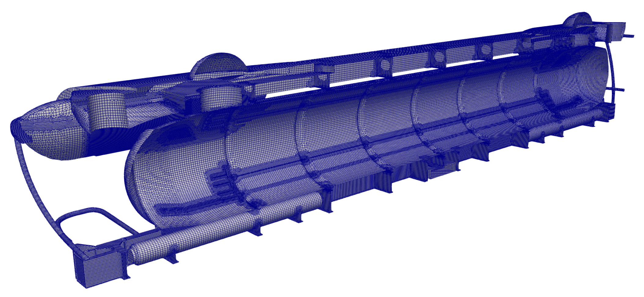
The paper is organised as follows. Section 2 presents the numerical analysis of the submarine; laying out flow equations and the numerical modelling approaches, describing the submarine that is the subject of the study, describing simulated conditions are shown in detail, describing the numerical simulation set up, and showing the numerical results. Section three contains a discussion of the obtained results, while section four gives a short conclusion of the work.

2. Numerical Analysis of Submarine Resistance

2.1. Numerical Model

The numerical model used in this work is based on a collocated Finite Volume (FV) approach for discretising the Reynolds Averaged Navier–Stokes Equations (RANSE). The software, called the Naval Hydro pack, is based on the open-source CFD software called foam–extend, a community driven fork of the OpenFOAM. The numerical model is developed with the aim of simulating large-scale, two-phase, incompressible, turbulent, and viscous flow with a free surface between the two phases, frequently encountered in the field of marine hydrodynamics. Under these assumptions, the governing flow equations are based on the volume continuity equation and the momentum conservation equations, as follows:

$$\nabla ·\mathbf{U}=0,$$

(1)

$$\frac{\partial u}{\partial t}+\nabla ·\left(\mathbf{U}\mathbf{U}\right)-\nabla ·\left({\nu }_e\nabla \mathbf{U}\right)=-\frac{1}{\rho }\nabla p_d,$$

(2)

where $\mathbf{U}$ stands for the velocity volume vector field, ${\nu }_e$ is the effective kinematic viscosity, $\rho$ is the density of the fluid, and $p_d$ stands for dynamic pressure defined as $p_d=p-\rho \mathbf{g}\mathbf{x}$. Here, p is pressure, $\mathbf{g}$ is gravitational acceleration vector, and $\mathbf{x}$ is the radii vector. In the present formulation, $\rho$ is discontinuous, being constant in two fluids and having a discontinuity across the free surface. The effective kinematic viscosity is defined as the sum of fluid kinematic viscosity and turbulent kinematic viscosity.

In this work, the interface is modelled using an implicitly re-distanced Level Set (LS) approach, modified to improve the conservation properties of the method [10]. The LS method is based on a sign distance, whose value represents the perpendicular distance to the free surface, The LS field $\psi$ is governed by the following equation [11]:

$$\frac{\partial \psi }{\partial t}+\nabla ·\left(\mathbf{c}\psi \right)-\psi \nabla ·\psi -b\nabla ·\left(\nabla \psi \right)=\frac{b\sqrt{2}}{ϵ}tanh\frac{\psi }{ϵ\sqrt{2}},$$

(3)

where b and $ϵ$ stand for the diffusion coefficient and width parameter, respectively. Vector $\mathbf{c}$ is a modified convective velocity field defined as $\mathbf{c}=\mathbf{U}+{\mathbf{w}}_1+{\mathbf{w}}_2$, where ${\mathbf{w}}_1$ and ${\mathbf{w}}_2$ are defined as:

$${\mathbf{w}}_1=\frac{b\sqrt{2}}{ϵ}tanh\left(\frac{\psi }{ϵ\sqrt{2}}\right)\nabla ϵ,$$

(4)

$${\mathbf{w}}_2=b\kappa \frac{\nabla \psi }{\nabla \left|\psi \right|},$$

(5)

and where $\kappa$ is the mean curvature of the free surface.

To render Equations (1) and (2) valid for both fluids, divided by an interface, jump conditions must be employed to account for the discontinuity of the density field. This is conducted by employing the Ghost Fluid Method (GFM), which yields discretisation schemes for different mathematical operators that are interface-corrected [12].These operators are derived by assuming the following jump conditions across the free surface:

• Discontinuity of the density field $\rho$:

  $$\left[\rho \right]={\rho }_a-{\rho }_w,$$

  (6)

  where $[.]$ stands for the jump operator, defined as the difference between the value infinitesimally close to the free surface on the air and water side. ${\rho }_w$ stands for the density of water, and ${\rho }_a$ for density of air. Note that the method can be used for any liquid–gas combination, as long as they are immiscible and have a sharp interface. Given the focus of this work, the liquid and gas will be assumed to be water and air, respectively, throughout the text.
• Continuity of the pressure field p, arising from the dynamic free surface boundary condition:

  $$\left[p\right]=0,$$

  (7)

  which neglects the surface tension of the free surface. This assumption is valid for large-scale flow phenomena predominant in the field of marine hydrodynamics.
• Continuity of the pressure gradient normalised by density, which is a result of applying the kinematic free surface boundary condition to the momentum equation [11]:

  $$\left[\frac{\nabla p}{\rho }\right]=0.$$

  (8)
  Applying the above equation to various discretisation schemes yields the interface-sensitised schemes for the pressure field. These eliminate the “spurious air velocity” problem, which is manifested in the phase-averaged approach that is more commonly used in numerical hydrodynamics. The reader is directed to [11] for more details.

The governing equations are closed using the k–$\omega$ SST turbulence model [13]. Time derivative terms in the governing equations are discretised with first-order accurate implicit Euler scheme. The convection term in the momentum equation is discretised using the Gauss theorem where the linear, upwind-biased interpolation is used to interpolate from cell-centres to face-centres. All diffusion terms are discretised using the Gauss theorem and central-differencing, with an over-relaxed approach for the non-orthogonal correction.

2.2. Description of the Submarine

The subject of this study is a touristic submarine designed to reach depths of up to 50 m, and to operate at speeds or currents of up to 3 knots. The pressure hull of the submarine will be made out of transparent acrylic tubes joined with steel rings into a continuous cylinder. Most of the submarine utility systems, such as compressed air systems, ballast tanks, compressed oxygen, propulsion systems, batteries, etc., are located outside of the pressure hull, within the exostructure and mask elements. For this reason, there are many hull elements that are outside of the aerodynamically shaped, cylindrical pressure hull. Figure 1 shows the visual representation of the submarine. The main particulars are listed in

Table 1. Main particulars of the submarine.

Length over all	$L_{OA}$	25.115 m
Maximal breadth	B	4.75 m
Depth	D	4.74 m
Draft while surfaced	T	3.42 m
Dry weight	m	142 tons

.

2.3. Simulated Conditions

The aim of this study is to give insight into the resistance properties of a submarine with intricate exostructure elements. For this purpose, the study attempts to quantify the contribution of the exostructure to the total resistance and attempts to bring that into relation with the conventional way of normalising resistance in naval architecture (force coefficients based on wetted surface). This is achieved by calculating resistance for three different geometries:

• Geometry 1: Smooth cylindrical hull, representing a simplified geometry of the pressure hull, Figure 2;
• Geometry 2: Cylindrical pressure hull with ring protrusions placed at 2.4 m intervals, with thickness of 240 mm and 60 mm height, Figure 3;
• Geometry 3: Full geometry of the pressure hull and exostructure, Figure 4.

In addition to the resistance differences between the above-listed geometries, the free surface effects are also investigated for Geometry 2 and Geometry 3. Simulations are performed at the design draft while surfaced, at a depth of 6 m (measured between the free surface and the top of the submarine), and at a depth of 40 m (effectively infinite depth). For Geometry 1, simulations are carried out for 6 and 40 m depth. Simulations are carried out for speeds ranging from 0.5 to 4.5 knots of speed.

Table 2. Test matrix.

Geometry No.	1	2	3
Speeds in knots	1.5, 3, 4.5	1.5, 3, 4.5	1.5, 3, 6
Froude numbers	0.05, 0.1, 0.15	0.05, 0.1, 0.15	0.05, 0.1, 0.2
Reynolds numbers	$1.94\times {10}^7$, $3.88\times {10}^7$, $5.81\times {10}^7$	$1.94\times {10}^7$, $3.88\times {10}^7$, $5.81\times {10}^7$	$1.94\times {10}^7$, $3.88\times {10}^7$, $7.75\times {10}^7$
Sailing depths	6 m, 40 m	0 m, 6 m, 40 m	0 m, 6 m, 40 m

shows the test matrix of conducted simulations and lists the depths and speeds tested for each geometry.

2.4. Description of Simulation Set Up

Despite the submarine being symmetric, the full domain is simulated due to possible large-scale vortex generation and shedding. The submarine is held at an even keel and fixed position in all simulations, not allowing motion due to hydrodynamic forces. The computational mesh is created using the cfMesh software, where the domain size is determined based on the size of the submarine, with $2L_{OA}$ in front and back of the submarine, $1L_{OA}$ on the sides, $3L_{OA}$ above and beneath the submarine. The total number of cells is:

• Geometry 1: 2,837,383 cells;
• Geometry 2: 2,853,694 cells;
• Geometry 3: 11,091,951 cells.

The discretised surface of the submarine is divided into seven different surface groups, called patches, to allow separate force calculations. The discretised surface and patch division are shown in Figure 4 and Figure 5. Figure 6 and Figure 7 show the sliced geometry of the submarine and the surface grid, where the structural elements can be better observed.

2.5. Numerical Results

Simulation results are shown in this section. Results are represented by the following values:

• $F_t$: Total resistance;
• $F_p$: Pressure resistance;
• $F_v$: Viscous resistance;
• $C_t=\frac{F_t}{1/2\rho S{V}^2}$: Total resistance coefficient;
• $C_p=\frac{F_p}{1/2\rho S{V}^2}$: Pressure resistance coefficient;
• $C_v=\frac{F_v}{1/2\rho S{V}^2}$: Viscous resistance coefficient.

where S is the dynamic wetted surface and V is the speed of the submarine in m/s. Dynamic wetted surface is the wetted surface measured while the submarine is in motion. Note that pressure resistance includes wave-making resistance.

Figure 8 shows the plotted results of all simulations. The legend denotes the geometry and depth of individual curves. Figure 9 shows the resistance results for Geometry 1 and 2 in isolation, for better visibility. The graphs show the absolute value of resistance. Figure 10, Figure 11 and Figure 12 show the resistance of individual submarine patches denoted in Figure 4 for the submarine sailing at the free surface, at 6 m depth, and 40 m depth, respectively. Here, negative values denote that the patch is contributing to resistance, and positive that it is reducing the resistance. Finally, resistance results are show in tabular form in

Table 3. Resistance results for the complete submarine geometry, Geometry 3.

Speed, kn	1.5			3			6
Fr	0.05			0.10			0.20
Depth, m	0	6	40	0	6	40	0	6	40
$F_t,N$	3374.8	4440.62	4407.86	12,432.37	17,036.13	16,650.25	51,241.67	66,722.5	64,331.01
$F_p,N$	3200.03	4221.6	4189.86	11,845.72	16,232.87	15,887.88	49,182.31	63,729.13	61,480.15
$F_v,N$	174.77	219.02	218	586.65	803.26	762.36	2059.37	2993.38	2850.87
$C_t\times {10}^3,-$	19.64	19.11	18.97	18.03	18.33	17.92	18.35	17.95	17.31
$C_p\times {10}^3,-$	18.62	18.17	18.04	17.17	17.47	17.1	17.62	17.15	16.54
$C_v\times {10}^3,-$	1.02	0.94	0.94	0.85	0.86	0.82	0.74	0.81	0.77
$S,m^2$	563.12	761.38	761.38	565.11	761.38	761.38	571.9	761.38	761.38

,

Table 4. Resistance results for the cylindrical pressure hull with ring protrusions, Geometry 2.

Speed, kn	1.5			3			4.5
Fr	0.05			0.10			0.15
Depth, m	0	6	40	0	6	40	0	6	40
$F_t,N$	774.92	705.25	674.41	3102.88	2780.04	2660.81	7348.8	6149.9	5879.6
$F_p,N$	693.07	600.71	572.78	2820.89	2409.24	2296.34	6787.78	5379.74	5127.37
$F_v,N$	81.85	104.54	101.63	281.99	370.8	364.47	561.01	770.17	752.23
$C_t\times {10}^3,-$	14.59	13.14	12.56	15.81	12.95	12.39	16.19	12.73	12.17
$C_p\times {10}^3,-$	13.05	11.19	10.67	14.38	11.22	10.7	14.95	11.14	10.61
$C_v\times {10}^3,-$	1.54	1.95	1.89	1.44	1.73	1.7	1.24	1.59	1.56
$S,m^2$	174.1	175.91	175.91	160.78	175.91	175.91	165.31	175.91	175.91

and

Table 5. Resistance results for the smooth cylindrical pressure hull, Geometry 1.

Speed, kn	1.5		3		4.5
Fr	0.05		0.10		0.15
Depth, m	6	40	6	40	6	40
$F_t,N$	296.86	292.09	1153.25	1091.43	2388.76	2331.96
$F_p,N$	144.05	140.35	604.53	545.42	1222.67	1175.99
$F_v,N$	152.82	151.74	548.72	546.01	1166.09	1155.97
$C_t\times {10}^3,-$	5.6	5.51	5.44	5.15	5.01	4.89
$C_p\times {10}^3,-$	2.72	2.65	2.85	2.57	2.56	2.47
$C_v\times {10}^3,-$	2.88	2.86	2.59	2.58	2.45	2.42
$S,m^2$	173.6	173.6	173.6	173.6	173.6	173.6

.

Figure 13 shows the free surface elevation during the simulation of the Geometry 3 sailing at the free surface, at 1.5 and 6 knots. The free surface is not disturbed at 1.5 knot due to the small Froude number, while a significant wave field is being generated at 6 knots. Figure 14 shows the dynamic pressure distribution in side view of Geometry 3, together with the free surface. Figure 15 shows streamlines from various viewpoints around Geometry 3, while sailing at 40 m depth. Figure 16 shows the dynamic pressure field for the three geometries while sailing at 40 m depth.

3. Discussion

3.1. Comparison of Resistance between Geometries

Resistance of the submarine (Geometry 3) is dominated by pressure resistance, with $C_p\times {10}^3$ ranging from 16.5 to 18.6; the viscous resistance only accounts for a little above 5% of the resistance, with $C_v\times {10}^3$ ranging from 0.7 to 1.0. This larger, atypical disparity between these two resistance components is caused by the relatively large wetted surface compared to the size of the vessel, and by the fact that there are numerous exostructure components exposed to the flow that are oriented perpendicular to it. Figure 10, Figure 11 and Figure 12 show that in all cases, the exostructure contributes most to the overall resistance of the hull, followed by the pressure hull. Despite its relatively small volume, the elements of the exostructure carry a significant portion of the overall resistance. This is further depicted by comparing the resistance of Geometry 3 and 2, where it can be observed that at 3 knots and 6 m depth, for example, Geometry 2 had only 16.4% of the resistance of Geometry 3; 83.6% of Geometry 3 resistance is generated by elements other than the pressure hull, which takes up most of the volume by far.

The resistance per unit wetted surface, expressed through resistance coefficients, was much higher for Geometry 3 and Geometry 2 compared to Geometry 1. Note that this effect is due to an increase in pressure resistance rather than viscous resistance. Indeed, the viscous resistance coefficient is lower for Geometry 3 and 2 compared to Geometry 1. This is due to the fact that a significant portion of the wetted surface of Geometry 3 and 2 do not experience shear flow. The numerous perpendicularly placed structural elements cause flow separation and re-circulation, reducing the amount of sheer flow next to the submarine’s surfaces. The absence of such elements in Geometry 1 means that the surface is exposed for the most part to sheer flow, as is most commonly the case in classical submarines or surface vessels. Despite a relatively small change in geometry between Geometry 1 and 2, the difference in resistance ranges from 111% to 152%, increasing with Froude number. This can be attributed to the perpendicular rings present in Geometry 2, disrupting the sheer boundary layer flow and causing the increase of pressure resistance. At the same time, the viscous resistance drops by around 30% to 40%. The changes that the rings, as well as other elements of the geometry, introduce to the dynamic pressure field are visible in Figure 16. Furthermore, Figure 15 shows that there are numerous regions of re-circulation.

Viscous resistance coefficient $C_v$ can be compared against the ITTC correlation line, which offers the empirically derived viscous resistance of a flat plate:

$$C_{ITTC}=\frac{0.075}{{(logRe-2.0)}^2},$$

(9)

where $Re$ stands for the Reynolds number, calculated as $Re=V{L}_{OA}/\nu$, where V stands for flow speed in meters per second, and $\nu$ stands for kinematic viscosity.

Table 6. Viscous resistance coefficients according to the ITTC correlation line.

Speed, kn	1.5	3	4.5	6
$C_{ITTC}\times {10}^3,-$	2.79	2.42	2.28	2.23

shows the viscous resistance coefficients as calculated using the above equation for the relevant speed range. Comparing these values to the ones presented in Table 3, Table 4 and Table 5, reveals that for Geometry 2 and 3 $C_v$ is lower than $C_{ITTC}$, indicating that the normalised viscous resistance is lower then that of a flat plate. For Geometry 1, the opposite is true and $C_v$ remains above $C_{ITTC}$ for all speeds by around 2% to 6%; these values are typical for streamlined shaped submarines and surface vessels, where the pressure viscous resistance (accounted for using the form factor k in most cases) causes the slight increase compared to the flat plate. For Geometries 2 and 3, the effective surface that is exposed to significant sheer flow is reduced and therefore viscous resistance is small compared to the total wetted surface. For this reason, the viscous resistance coefficient is reduced.

3.2. Free Surface Effects

For Geometry 2, the resistance increases as depth decreases. The largest resistance was observed when sailing at the free surface. At the free surface, the object has to overcome additional wave-making resistance, which is absent at great depths, as shown by Chen et al. [8] and in Figure 9. The increase in resistance between 40 and 6 m depth was relatively small, below 2%; the increase between 40 and 0 m of depth was larger than 10%.

Contrary to what is expected, the submarine (Geometry 3) showed lower resistance when sailing at the free surface (Table 3), compared to sailing at 40 m of depth, which is effectively infinite depth. However, looking at the results in Table 3 more carefully, it can be observed that the total resistance coefficient $C_t$ was higher at the free surface compared to sailing at 40 meters of depth. This means that the resistance per unit of wetted surface is indeed higher when sailing at the free surface. However, this difference is relatively small compared to Geometry 2—here the relative difference between resistance coefficients at 0 and 40 m of depth was 15% at 1.5 knots, 27% at 3 knots, and 33% at 4.5 knots, while for Geometry 3 it was only 3%, 2%, and 6%, respectively. Note that the difference is expected to increase with increasing Froude number, for conventional submarines. Moreover, for Geometry 3 the resistance coefficient is smaller at the free surface compared to 6 m depth at the speed of 3 knots.

This apparent departure of results for Geometry 3 from expected trends can be explained by the fact that for the submarine vehicle studied in this project, the geometry that is outside during sailing at the free surface, is not necessary equivalent in its normalised hydrodynamic qualities to the portion of the submarine that remains under water. Indeed, the transversal beam elements below the fairings (see the green-coloured structural elements above the middle part of the pressure hull in Figure 6), which are outside when sailing at the free surface, are expected to exhibit larger pressure resistance coefficients than, e.g., the pressure hull or the battery pack. Thus, the increase in resistance due to wave resistance does not manage to compensate the reduction of resistance due to the reduced overall resistance coefficient of the surface that remains underwater.

Note that the results at 6 m of depth in Table 3, show an expected increase in resistance for all speeds compared to the resistance at large depths. This shows that when the entire submarine is under water, the resistance increases when sailing closer to the free surface.

Additional corroboration of the above conclusion can be found in forces calculated on individual patches. From Table 3, it can be seen that the difference in total resistance at 0 and 40 m of depth is almost entirely composed of the difference in forces acting on patch “fairings”. This patch is completely dry when sailing at the free surface, and does not contribute to hydrodynamic resistance. This can be observed in Figure 13 and Figure 14, where the side view of the submarine and perspective view are shown sailing at the free surface at different speeds.

4. Conclusions

A numerical RANS study of a submarine resistance is presented in this study. The aim of this work is to investigate the influence of exostructural elements on the resistance of the submarine and compare it against the resistance of the pressure hull, the largest element of the submarine. In addition, the effect of the free surface on the resistance of such a submarine is investigated, showing that when sailing at the free surface, the submarine has lower resistance compared to sailing at large depth, which goes against expectations. The study shows that exostructural elements have a significant impact on submarine resistance, more than doubling its resistance compared to the resistance of the smooth pressure hull.

References

1. Jiao, H.; Fu, W.; Zhang, L.; Zhao, C.; Zheng, Z. Simulation research and optimization design on towed system of manned submersible. In Proceedings of the 2018 IEEE 8th International Conference on Underwater System Technology: Theory and Applications (USYS), Wuhan, China, 1–3 December 2018. [Google Scholar]
2. Jiang, Z.; Lu, B.; Wang, B.; Cui, W.; Zhang, J.; Luo, R.; Luo, G.; Zhang, S.; Mao, Z. A Prototype Design and Sea Trials of an 11,000 m Autonomous and Remotely-Operated Vehicle Dream Chaser. J. Mar. Sci. Eng. 2022, 10, 812. [Google Scholar] [CrossRef]
3. Wei, Z.F.; Wang, M.Y.; Yu, Q.; Yang, S.L. A Design of Resistance Optimization System for Unmanned Submersible Vehicle Based on Response Surface Method. In Proceedings of the 2014 International Conference on Mechanics and Civil Engineering; Chen, W., Wu, X., Xu, J., Eds.; AER-Advances in Engineering Research; Atlantis Press: Amsterdam, The Netherlands, 2014; Volume 7, pp. 128–133. [Google Scholar]
4. Kotb, M.A.; Banawan, A.; Ahmed, Y.M. Flow field characteristics past a slow speed tourist submarine and their environmental impacts. In Proceedings of the 7th International Conference on Role of Engineering towards a Better Environment, Alexandria, Egypt, 20–22 December 2008. [Google Scholar]
5. Phillips, A.; Furlong, M.; Turnock, S.R. The use of computational fluid dynamics to assess the hull resistance of concept autonomous underwater vehicles. In Proceedings of the OCEANS 2007—Europe, Aberdeen, UK, 18–21 June 2007. [Google Scholar] [CrossRef] [Green Version]
6. Khan, S.A.; Fatepurwala, M.A.; Pathan, K.N.; Dabeer, P.S.; Baig, M.A.A. CFD analysis of human powered submarine to minimize drag. Int. J. Mech. Prod. Eng. Res. Dev. 2018, 8, 1057–1066. [Google Scholar] [CrossRef]
7. Karim, M.M.; Rahman, M.M.; Alim, M.A. Performance of SST k-ω turbulence model for computation of viscous drag of axisymmetric underwater bodies. Int. J. Eng. Trans. B Appl. 2011, 24, 139–146. [Google Scholar]
8. Chen, J.; Lv, B.; Peng, L.; Huang, B. Study on resistance characteristics of submarine near water surface. MATEC Web Conf. 2022, 355, 01002. [Google Scholar] [CrossRef]
9. Ćorak, M.; Šperanda, Z.; Čokić, J.; Parunov, J. Structural analysis of tourist submarine with acrylic hull. In Sustainable Development and Innovations in Marine Technologies; Guedes Soares, S., Ergin, S., Eds.; CRC Presss: London, UK, 2022; pp. 381–387. [Google Scholar]
10. Vukčević, V.; Jasak, H. A Conservative Level Set Method for Interface Capturing in Two-Phase flows. In Proceedings of the 11th World Congress on Computational Mechanics (WCCM XI), Barcelona, Spain, 20–25 July 2014; pp. 1082–1095. [Google Scholar]
11. Vukčević, V. Numerical Modelling of Coupled Potential and Viscous Flow for Marine Applications. Ph.D. Thesis, Faculty of Mechanical Engineering and Naval Architecture, University of Zagreb, Zagreb, Croatia, 2016. [Google Scholar]
12. Vukčević, V.; Jasak, H.; Gatin, I. Implementation of the Ghost Fluid Method for free surface flows in polyhedral Finite Volume framework. Comput. Fluids 2017, 153, 1–19. [Google Scholar] [CrossRef]
13. Menter, F.R. Two-Equation Eddy-Viscosity Turbulence Models for Engineering Applications. AIAA J. 1994, 32, 1598–1605. [Google Scholar] [CrossRef]
Figure 1. Visual representation of the submarine.
Jmse 10 01542 g001
Figure 2. Geometry 1: Smooth cylindrical hull, representing a simplified geometry of the pressure hull.
Jmse 10 01542 g002
Figure 3. Geometry 2: Cylindrical hull with ring protrusions, representing the geometry of the pressure hull with rings.
Jmse 10 01542 g003
Figure 4. Geometry 3: Geometry of the pressure hull and exostructure used in the CFD simulation. The geometry is divided into a number of different patches denoted on the figure.
Jmse 10 01542 g004
Figure 5. Geometry 3: Geometry of the pressure hull and exostructure used in the CFD simulation, bottom view.
Jmse 10 01542 g005
Figure 6. Geometry 3: Sliced view of the geometry.
Jmse 10 01542 g006
Figure 7. Geometry 3: Sliced view of the discretised surface geometry of the submarine.
Jmse 10 01542 g007
Figure 8. Total resistance results for all cases.
Jmse 10 01542 g008
Figure 9. Total resistance of the smooth and simplified pressure hull, Geometry 1 and 2.
Jmse 10 01542 g009aJmse 10 01542 g009b
Figure 10. Resistance of individual patches of Geometry 3 when sailing at the free surface (0 m depth).
Jmse 10 01542 g010
Figure 11. Resistance of individual patches of Geometry 3 when sailing at depth of 6 m.
Jmse 10 01542 g011
Figure 12. Resistance of individual patches of Geometry 3 when sailing at depth of 40 m.
Jmse 10 01542 g012
Figure 13. Free surface elevation at 1.5 and 6 knots for Geometry 3 sailing at the free surface.
Jmse 10 01542 g013
Figure 14. Pressure distribution and free surface geometry at 1.5 and 6 knots for Geometry 3 sailing at the free surface.
Jmse 10 01542 g014
Figure 15. Streamlines around the submarine when sailing at 3 knots speed at 40 m depth.
Jmse 10 01542 g015
Figure 16. Pressure distribution for Geometry 1, 2, and 3, from left to bottom right. Pressure is shown at 4.5 knots for Geometry 1 and 2, and at 3.0 knots for Geometry 3.
Jmse 10 01542 g016