Wave Height Reduction Inside Pohang New Port, Korea, Due to the Construction of a Detached Breakwater

Abstract

The effect of a detached breakwater, which was constructed to improve harbor tranquility inside Pohang New Port, was examined through the comparison of wave data measured before and after the construction of the breakwater. The observation data showed that the wave energy was effectively reduced by the breakwater, although the wave height measured outside the breakwater was higher after its construction. The wave energy was reduced in all of the measured wave-propagating directions, but it was also observed that the breakwater became less effective in protecting against northeastwaves than in protecting against NNE waves. The BOUSS-2D Boussinesq-type wave model was employed to analyze the pattern of wave propagation, showing that, before the breakwater’s construction, NE waves could directly enter the port, increasing the wave energy inside the port. After the breakwater’s construction, simulations showed that the detached breakwater effectively blocked the waves approaching the port from both the NNE and NE directions, although the wave heights of the waves from the extreme NE direction inside the port increased. Considering that the estimated probability of failing to preserve the port tranquility was only 0.2–0.5% for these extreme NE waves, it was concluded that no secondary structures were necessary, and the existing breakwater was sufficient for the protection of the port.

1. Introduction

Since the construction of Pohang New Port inside Yeongil Bay in the southeastern end of the Korean Peninsula in 1985, questions have been raised regarding the harbor’s tranquility because downtime occurs frequently, which might lower the port’s operation rate. Unexpected downtime due to harbor agitation may interrupt port operation and reduce throughput, and harbors with complex topologies and layouts are prone to experiencing severe agitation and downtime problems that are difficult to predict [1]. Therefore, studies have been performed to determine the factors that affect the tranquility of a harbor (e.g., [2]). For example, knowledge of short-period waves with wave periods less than 30 s, such as wind waves and swells, is an essential prerequisite for the planning and design of harbor protection structures [3], and numerical models have been employed to assess wave agitations induced by short waves in ports [4,5,6]. On the other hand, it has been suggested that long waves, including infragravity waves, might also be important factors that affect the harbor operation rate even when the harbor offers good protection against short waves [7,8,9], and low-frequency motions via harbor resonance could also cause agitations inside a harbor [10]. In addition, it was reported that the vertical movement of a vessel at berth was mainly determined by the swell energy inside the port basin, but the horizontal movement was strongly correlated with the low-frequency band energy [11].

In the case of Pohang New Port, it is difficult to determine the exact causes of the frequent downtimes, as its initial design changed due to port expansion, which meant that the combined effects of short waves, infragravity waves, and natural oscillation had to be considered. For example, it was suggested that the contribution of long waves and the natural oscillation period could be also considerable [1]. On the contrary, there have been research results that support the concept that short gravity waves are still the major cause of the downtime in Pohang New Port [12,13,14], and a detached ~700 m long breakwater with 15 caissons was constructed from October 2018 to December 2020 according to these study results [15,16]. Therefore, the present study was designed to investigate the effectiveness of the detached breakwater in improving the harbor tranquility and thus to confirm the research results that suggested short waves are the main cause for the downtime in Pohang New Port. Previously, a similar experiment was conducted to analyze the effectiveness of a detached breakwater [17]. According to this study, the harbor tranquility was improved after a detached breakwater was constructed. However, the accuracy of the results was questioned [17] because the wave data outside the port were measured at the entrance of Yeongil Bay.

To resolve this problem, in the present study, we employed wave observation data measured at additional stations inside Yeongil Bay, both before and after the construction of the breakwater. The new wave data in this study were measured at three additional stations (W1, W6, and W7 in Figure 1). Therefore, one of the advantages of the present study is that the waves were measured (just) offshore of the detached breakwater, meaning that a direct comparison with the waves inside Pohang New Port increased the accuracy of the results. The most significant contribution of this study is that the harbor tranquility was closely investigated based on field wave data obtained from the observations in both periods before and after the construction of the detached breakwater. Therefore, we were able to examine the effect of the breakwater on the tranquility inside the port under various wave conditions that occurred in the real field. To the best of the authors’ knowledge, most of the previous studies that investigated harbor tranquility were based on physical and numerical model experiments, laboratory experiments, or the application of artificial intelligence approaches. Field observation data were used in some previous studies, but only for limited times of the observational periods at daily scales. In this study, the results from the analysis of field data removed the uncertainties that could arise from the simulations that used models and AI approaches. The variety of the wave conditions during the experimental periods could also offer inferences for extreme cases through statistical data. In addition to the analysis of the observation data, a Boussinesq-type wave propagation model was used to conduct numerical experiments to support the observational results by investigating the mechanism during the courses of wave propagation before and after the construction of the breakwater.

The purpose of this study was to analyze the rate of the reduction of wave height inside Pohang New Port due to the construction of a detached breakwater by using improved wave observation data and also by using a phase-resolving wave model that is capable of simulating the effects of wave refraction and diffraction in the complicated topography near the port. In this study, we also aimed to investigate the effect of the breakwater by examining the reduction rate according to the wave propagation direction and thus to provide precedent data in designing future structures in similar environments.

2. Materials and Methods

2.1. Study Site

Figure 1 shows the map of Yeongil Bay, captured from Google Earth, located in the southeast of the east coast of the Korean Peninsula, which is located in Northeast Asia. Yeongil Bay faces northeast with a mouth of ~10 km. Therefore, the waves that approach from the NE direction could reach the inner part of the bay and even affect the tranquility inside Pohang New Port [18]. As shown in Figure 1c, Pohang New Port was designed to protect the port from waves that mainly approach in the NE direction. However, the frequent downtime remained problematic in terms of the port’s operation, which was unusual compared to the cases of other trading ports in the Republic of Korea.

As introduced in Section 1, previous research results have supported the concept that short gravity waves are the major cause for downtime in Pohang New Port, suggesting that harbor tranquility would be improved if the intrusion of short waves into the port was effectively prevented [12,14] and proposing that the target wave height to reach the desired harbor tranquility is 0.3 m [13]. As a measure to maintain the target wave height inside the port, it was suggested that a detached breakwater could be constructed outside the port to block approaching waves. Harbor breakwaters are usually constructed parallel to the shoreline near the edge of the surf zone to reduce the wave energy and protect the shore [19,20]. However, detached breakwaters have also been commonly constructed outside harbors to reduce the energy of waves that propagate to the harbor [21], along with other devices [22]. As a result, a detached, ~700 m long breakwater with 15 caissons was constructed from October 2018 to December 2020 [15,16]. In a previous study, the effect of the detached breakwater was investigated [17], and it was shown that the harbor tranquility was improved after the construction of the breakwater, as the frequency of the measured wave height exceeding the target wave height of 0.3 m clearly decreased. However, questions arose regarding the accuracy of the results of [17], because the wave data outside the port were measured at the entrance of Yeongil Bay. Due to the long distance from the wave station located at the bay entrance (W0 in Figure 1), the comparison with the wave data measured inside the port lowered the credibility of the analysis results. For example, the data in [17] showed that the breakwater was effective against waves in all directions measured at the bay entrance, W0. However, as shown in Figure 1, the course of wave propagation is varied inside Yeongil Bay, and waves from specific directions can successfully intrude into Pohang New Port, which implies that the effectiveness of the detached breakwater depends on the direction of the wave propagation.

2.2. Wave Measurement

Because Yeongil Bay is surrounded by land, the wave climate inside the bay is usually calmer than that outside the bay. However, waves could become harsh enough to cause severe coastline erosion in Yeongildae Beach when severe storm waves approach the site, even though the beach is located in the western corner of the bay [23]. Pohang New Port was constructed in 1985 at the southwest end of Yeongil Bay, as shown in Figure 1c, and the figure also shows the seven locations where waves were measured. An AWAC (Acoustic Wave And Current profiler) was installed on the sea bed at the entrance of Yeongil Bay (W0), as this is where waves were measured outside Pohang New Port in [17]. In this study, wave observations were carried out in W1, where an AWAC was installed on the sea bed ~1.2 km offshore from the head of the detached breakwater in the NE direction to measure the significant wave height ($H_{m0}$), peak wave period ($T_p$), and peak wave direction ($D_p$) every 30 min. Because an AWAC uses acoustic sensors to directly detect the wave surface elevation, it generally provides eave data with higher accuracy compared to a pressure transducer, which indirectly measures the surface elevation by converting the pressure time series using transfer functions [24]. During stormy conditions with strong wind, however, the white-capping of the waves disturbs the acoustic sensors, which may lower the accuracy of the AWAC measurements. In the case of W1, the AWAC was located inside the bay, and the wind energy was reduced as it was blocked by the land surrounding the bay, securing the validity of the AWAC data during most of the observational periods. The AWAC was used to measure the wave data from 21 May 2018. Before then, a Directional Waverider buoy from Datawell Inc. was moored at the same location, W1, to observe the wave conditions for ~9 months from 15 October 2008 to 12 July 2009, and the data during this period were also used in this study. Inside Pohang New Port, pressure sensors and a WTG (Wave and Tide Gauge) were deployed to measure $H_{m0}$ and $T_p$ at the four stations (W2, W3, W4, and W5), and their data were available during the same time periods, with the data from W1 being used for comparison. In addition to these stations inside the port, wave data were also measured using a pressure sensor and a WTG in the nearshore of Dogu Beach (W6) located in the southeast corner of Yeongil bay ~1.4 km in front of the beach. Similarly, another WTG was deployed in the west corner of the bay (W7) ~1.0 km in front of Yeongildae Beach. Due to these wave measurements in W6 and W7, the changes in the wave environment before/after the detached breakwater construction could be observed over the wider area inside Yeongil Bay. The wave data in W6 and W7 were measured from 21 May 2018, and thus, were not available in 2008 and 2009. The locations of the wave sensors, measuring periods, and speculations of the instruments are listed in

Table 1. List of observational instruments, locations, installation depths, and measuring frequency.

Station	Locations (Lat., Lon.)	Depth (m)	Instrument	Measuring Period	Measuring Frequency (Hz)
W0	36°05′21.90″ N 129°28′21.20″ E	D.L. (−)24.5	AWAC	21 May 2018–9 May 2020	2
W1	36°02′16.34″ N 129°27′12.03″ E	D.L. (−)22.0	Directional Waverider buoy	15 October 2008–12 July 2009	1.28
			AWAC	21 May 2018–9 May 2020	2
W2	36°00′46.30″ N 129°25′05.60″ E	D.L. (−) 8.5	WTG	15 October 2008–9 May 2020	2
W3	36°01′00.10″ N 129°24′58.00″ E	D.L. (−)11.0	WTG	15 October 2008–9 May 2020	2
W4	36°00′42.70″ N 129°24′45.30″ E	D.L. (−)10.0	WTG	15 October 2008–9 May 2020	2
W5	36°00′58.20″ N 129°24′36.10″ E	D.L. (−) 9.7	WTG	15 October 2008–9 May 2020	2
W6	36°00′21.15″ N 129°26′39.83″ E	D.L. (−)12.5	WTG	21 May 2018–9 May 2020	2
W7	36°03′22.65″ N 129°23′25.86″ E	D.L. (−) 8.5	WTG	21 May 2018–9 May 2020	2

.

As previously described, the effect of the detached breakwater was examined by separating the periods of wave measurements into two groups—before and after the construction of the breakwater. The 1st~6th caissons were placed between 15 October 2018 and 14 January 2019, and the 12th caisson was placed by 6 August 2019. In the present study, therefore, the period before construction (hereafter, BC) was set to the wave measurements that were conducted before 13 February 2019 when the 1st~6th caissons were placed (before the 7th caisson was placed), and the period after construction (hereafter, AC) was set to after 6 August 2019, when the 12th caisson was placed. The starting time of BC was set to 15 October 2008, when the observation in W1 started, and the ending time of AC was set to 9 May 2020. Therefore, two separate time periods were included in BC, as the first started from 15 October 2008 to 12 July 2009, during which the Directional Waverider buoy was installed in W1; this period lasted for 271 days. This first period of BC is abbreviated as BC01 hereafter. In BC01, the wave measurements were available at five (W1, W2, W3, W4, and W5) out of a total of eight stations. The second period in BC was from 21 May 2018 to 13 February 2019, which lasted for 269 days (hereafter, BC02). In BC02, the data in W2 were of poor quality, with a missing period of 85 days, which was excluded from the analysis. The AC period comprised 278 days from 8 August 2019 to 9 May 2020, and good-quality wave data were available at all measuring stations. The observational periods in BC (hereafter, BC refers the period that includes both BC01 and BC02) and AC are listed in

Table 2. List of the observation periods.

	Period	Data Availability
Before construction (BC) of the detached breakwater	15 October 2008–12 July 2009 (271 days, BC01)	Avail.: 5 station N.A.: 3 stations (W0, W6, W7)
	21 May 2018–13 February 2019 (269 days, BC02)	Avail.: 7 station N.A.: 1 station (W2)
After construction (AC) of the detached breakwater	6 August 2019–9 May 2020 (278 days, AC)	Avail.: 8 station N.A.: 0 station

.

In Figure 2, $H_{m0}$, measured in W1 and W3, is plotted for both BC and AC to compare the wave height outside and inside Pohang New Port. The value of $H_{m0}$ measured in BC01 is shown in Figure 2a, whereas the data measured in BC02 are shown in Figure 2b. The maximum $H_{m0}$ measured in W1 was 3.4 m in BC on 26 April 2009 and 4.8 m in AC on 22 September 2019, showing that it was higher in AC by ~1.4 m. In BC, there were ~168 h in which there were high wave conditions in which $H_{m0}$ in W1 was greater than 2 m, and in AC, there were ~332 h. Considering that the BC period was longer (540 days) than the AC period (278 days), it was found that the wave conditions were more energetic during AC. In contrast, the maximum $H_{m0}$ measured in W3 was 0.98 m in BC on 26 April 2009 and 0.64 m in AC on 22 September 2019, showing that it was higher in BC by ~0.34 m. In addition, in BC, there were ~183 h in which $H_{m0}$ was higher than 0.5 m in W3, and this was a much shorter time in AC, as it was ~10 h. Considering that the wave condition was generally higher in AC outside the port, the shorter period in which $H_{m0}$ was greater than 0.5 m in AC indicates that the detached breakwater clearly reduced the wave height inside the port. In Figure 2, the waves measured in W1 were used as the data outside the port instead of those measured in W0, and the reason for this is described in Section 3.

2.3. Selection of Wave Events

In order to examine the effect of the detached breakwater more closely, wave events were selected to filter out the calm wave conditions in which the breakwater effect could not be clearly observed because the wave energy was low both outside and inside the port. The wave events were selected by considering two conditions. The first was that $H_{m0}$ should be higher than 1 m in W1. The second condition was that the time in which $H_{m0}$ was greater than 1 m should last for at least 12 h so as to exclude inconsistent data. The number of selected wave events was 38 in BC and 27 in AC, the total time that corresponded to these wave events was 1150 h in BC and 1091 h in AC, and the time required for statistics was secured sufficiently. In Figure 3, time variations in wave height in W1 and W3 and wave direction in W1 are compared between the wave event examples selected in BC and AC. In both cases, the example events were selected as they had the maximum wave heights during each period. Therefore, for BC, a period of two days from 26 April 2009 was chosen as the example event. During this period, the $H_{m0}$ value in W1 increased to a maximum of ~3.4 m, and the $H_{m0}$ value in W3 increased to ~1.0 m. The wave direction range was N15°E~N50°E, showing that the waves generally approached in the NNE and NE directions, as these are the primary wave propagation directions in this region. For AC, a period of four days from 21 September 2019 was chosen as the example event; the $H_{m0}$ value in W1 increased to its maximum value of ~4.8 m, and the $H_{m0}$ value in W3 increased to ~0.6 m. The wave direction range was N40°E~N60°E, showing that the waves generally approached in the NE direction during this storm period.

2.4. Numerical Model Experiment

The BOUSS-2D wave model was employed to conduct numerical experiments to understand the results from the observational data. The observation results showed the breakwater reduced the wave energy inside the port through a comparison of wave height measurements between BC and AC. However, this comparison could not provide the detailed ways in which the reductions actually occurred, which would require additional numerical experiments to understand the processes of wave transformation. The BOUSS-2D wave model was developed based on the non-linear Boussinesq equations [25], and the background of the model is described as follows. The classical form of the Boussinesq equations for wave propagation over water of variable depth was derived by [26], and the equations were restricted to relatively shallow water depths ($h<\mathrm{L}/5$ with $h$ = water depth and $\mathrm{L}$ = wave length). Nwogu [27] extended the range of applicability of the Boussinesq-type equations to deeper water. Despite this improvement, these equations were based on the assumption that wave heights are much smaller than the water depth. This limited the ability of the equations to describe highly non-linear waves in shallow water and led to a fully non-linear form of equations that are useful for the simulation of asymmetric waves in shallow water, wave-induced currents, wave setup, and wave–current interaction [28]. Then, Nwogu [29] extended the fully non-linear form of Boussinesq equations to the surf zone to consider the turbulence generated by breaking waves and the effect of bottom friction. These modified equations were able to simulate most of the hydrodynamic phenomena in the coastal regions and harbor basins, which included shoaling, refraction, diffraction, reflection, bottom friction, wave–wave and wave–current interactions, wave-induced currents, and wave breaking and runup. The BOUSS-2D model has been successfully applied to simulate wave diffraction in the lee of coastal structures and wave propagation over relatively steep slopes.

BOUSS-2D equations are depth-integrated equations for the conservation of mass and momentum for non-linear waves propagating in shallow and intermediate water depths. They can be considered to be perturbations from shallow-water equations, which are often used to simulate tidal flows in coastal regions. For short-period waves, the horizontal velocities are no longer uniform over depth, and the pressure is non-hydrostatic. The vertical profile of the flow field is obtained by expanding the velocity potential, Φ, as a Taylor series for an arbitrary elevation, $z_{\alpha }$, in the water column. For waves with length, L, much longer than the water depth, $h$, the series is truncated at the second order, resulting in a quadratic variation in the velocity potential over depth:

$$\mathsf{\Phi }\left(\mathrm{x},\mathrm{z},\mathrm{t}\right)={\mathsf{\varphi }}_{\alpha }+{\mathsf{\mu }}^2\left(z_{\alpha }-\mathrm{z}\right)\left[\nabla {\mathsf{\varphi }}_{\alpha }·\nabla h\right]+\frac{{\mu }^2}{2}\left[{\left(z_{\alpha }+h\right)}^2-{\left(z+h\right)}^2\right]{\nabla }^2{\mathsf{\varphi }}_{\alpha }+O\left({\mu }^4\right)$$

(1)

where ${\mathsf{\varphi }}_{\alpha }=\mathsf{\Phi }\left(\mathrm{x},z_{\alpha },\mathrm{t}\right)$, $\nabla =\left(\partial /\partial \mathrm{x}, \partial /\partial \mathrm{y}\right)$, and $\mathsf{\mu }=h/\mathrm{L}$ is a measure of frequency dispersion. The horizontal and vertical velocities are obtained from the velocity potential as:

$$\mathrm{u}\left(\mathrm{x},\mathrm{z},\mathrm{t}\right)=\nabla \mathsf{\Phi }=u_{\alpha }+\left(z_{\alpha }-z\right)\left[\nabla \left(u_{\alpha }·\nabla h\right)+\left(\nabla ·u_{\alpha }\right)\nabla h\right]+\frac{1}{2}\left[{\left(z_{\alpha }+h\right)}^2-{\left(z+h\right)}^2\right]\nabla \left(\nabla ·u_{\alpha }\right)$$

(2)

$$\mathrm{w}\left(\mathrm{x},\mathrm{z},\mathrm{t}\right)=\frac{\partial \mathsf{\Phi }}{\partial \mathrm{z}}=-\left[u_{\alpha }·\nabla h +\left(\mathrm{z}+h\right)\nabla ·u_{\alpha }\right]$$

(3)

where $u_{\alpha }=\nabla \mathsf{\Phi }{|}_{z_{\alpha }}$ is the horizontal velocity at z =$z_{\alpha }$. Given a vertical profile for the flow field, the continuity and Euler (momentum) equations can be integrated over depth, reducing the three-dimensional problem to two dimensions. For more detailed information regarding the BOUSS-2D model, readers are referred to the manual in [25].

In this study, the BOUSS-2D model was set up in a rectangular grid system using the staggered method by calculating the time-varying surface elevation and horizontal velocities at the grid nodes. The computational domain around Pohang New Port is shown in Figure 4. A rectangular domain with a size of 6.8 km by 6.0 km was set up by rotating the domain to the NE direction so that the outer open boundary could face $\mathrm{N}40°\mathrm{E}$ (Figure 4a). This was because the majority of the waves approach in the NNE and NE directions in this region, and the input wave directions forced along the open boundary could range within $\pm 30°$, which is important for the stability of the model runs. The $\mathsf{\Delta }\mathrm{x}$ and $\mathsf{\Delta }\mathrm{y}$ of each grid was 5 m and set uniformly in the whole domain; thus, a total of 1360 grid points were allotted in the $\mathrm{x}$-direction (parallel to detached breakwater), and 1200 grids were allotted in the $\mathrm{y}$-direction.

The model was run for two different cases, representing the wave conditions in BC and AC, respectively. The two cases were the same as the selected events shown in Figure 3. That is, the model was run from 05:30 on the 26 to 21:30 on the 27 April 2009 for BC and from 07:00 on the 22 to 21:00 on the 23 September 2019 for AC. The BOUSS-2D model is not stable when used with waves of periods shorter than 8 s, meaning that the two cases were run for the times during which the observed periods were longer than 8 s. As it was not practical to continuously run BOUSS-2D for the whole time of 38–40 h, which had varying wave conditions, as shown in Figure 3, the experiment was conducted by running the model at every hour by specifying the directional spectra that represented the wave conditions at the corresponding time. In the case of BC, for example, the model was run 39 times, corresponding to each hour from 05:30 on the 26 to 21:30 on the 27 April 2009, with the model being forced to be determined from the data measured at each hour. Individual runs were simulated for 3900–4000 s until a stable condition was reached with $\mathsf{\Delta }\mathrm{t}$ = 0.15 s. These numerical experiments were designed to understand the course of wave energy reduction between BC and AC through model validation via comparisons with observational data. The results are discussed in Section 3.2 and Section 4.

3. Results

3.1. Observational Data

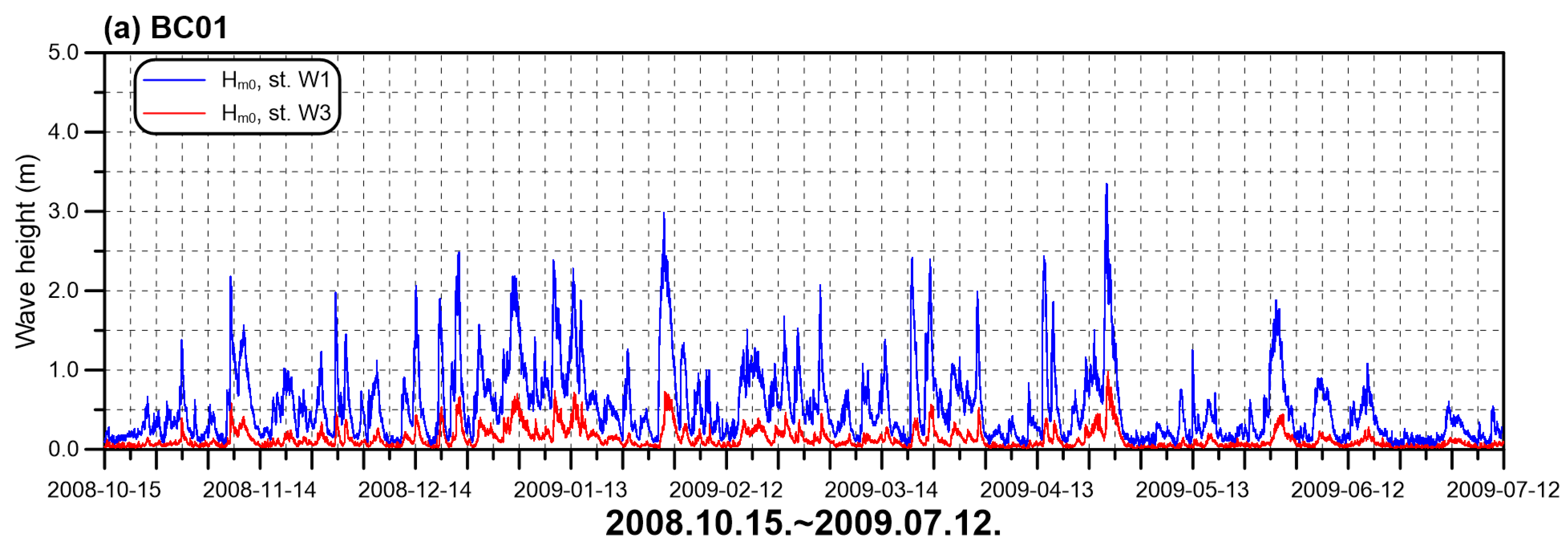
The number of wave events that consistently had wave heights greater than 1 m for at least 12 h was 38 in BC and 27 in AC, as described in Section 2. The selected events generally corresponded to the times when high waves, including storms, were present in Yeongil Bay, and $H_{m0}$ displayed increasing and decreasing patterns during these periods, as shown in Figure 3. 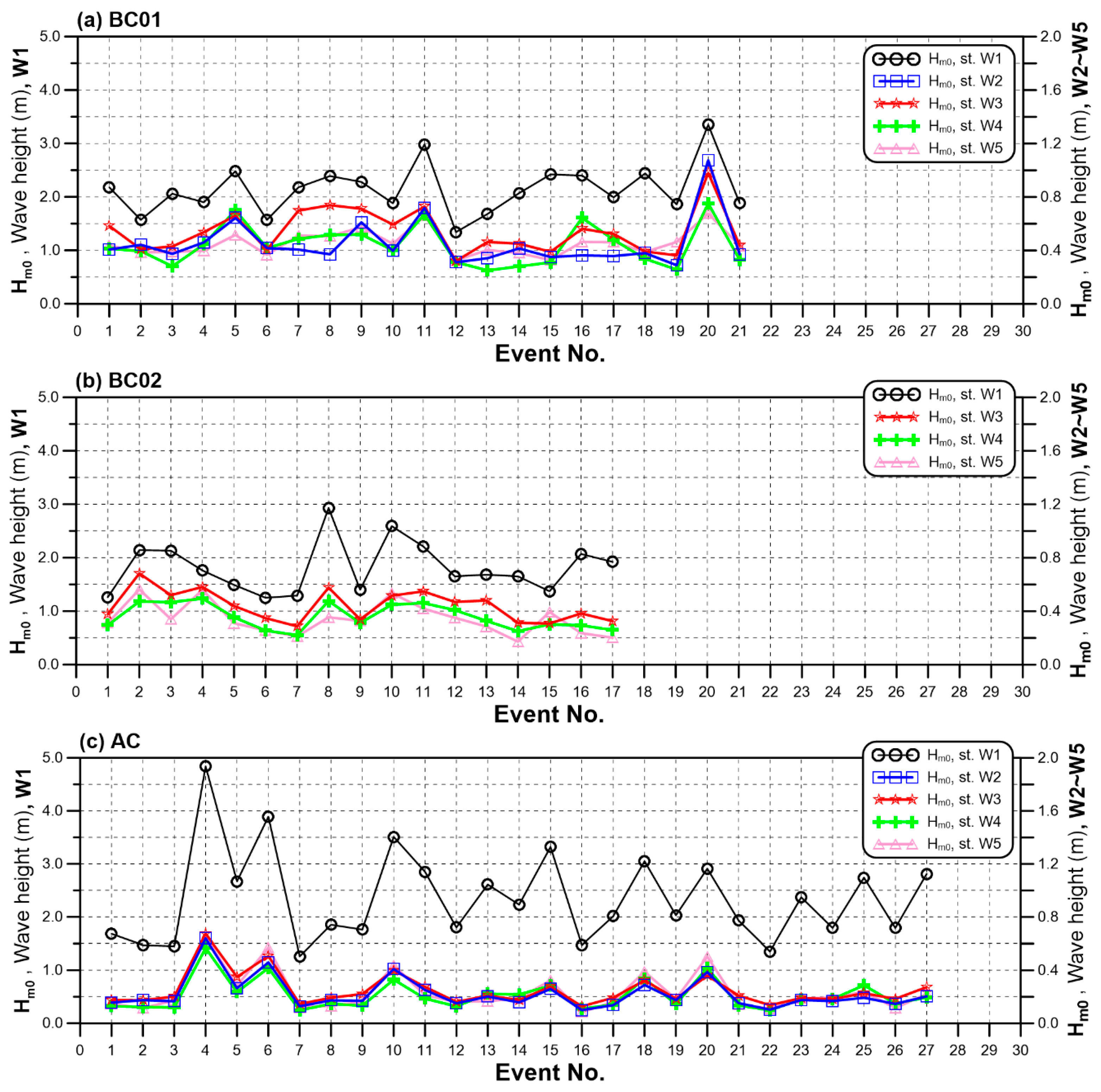Therefore, there was a time when the $H_{m0}$ value became the maximum, and the $H_{m0}$ value at this time was selected as the representative value for each event. In Figure 5, the maximum $H_{m0}$ values of all of the events are compared between W1 (outside Pohang New Port) and W2, W3, W4, and W5 (inside Pohang New Port) in BC and AC. 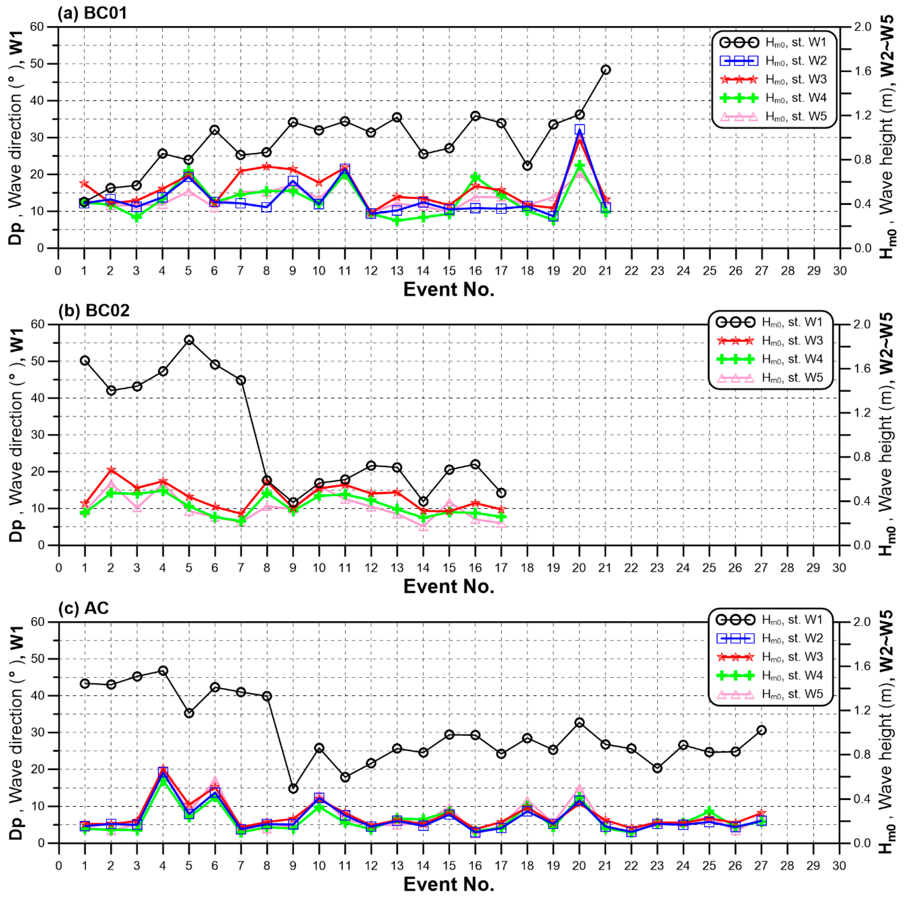Similarly, the representative values for the wave propagation direction, $D_p$, were selected at the same time at which the maximum $H_{m0}$ values for the corresponding events were observed. In Figure 6, the representative $D_p$ value measured in W1 is compared with the $H_{m0}$ value in W2, W3, W4, and W5.

In the case of wave height, the $H_{m0}$ varied with the wave events and showed similar patterns at all stations, as when the $H_{m0}$ value was high inside the port (W2, W3, W4, and W5), the $H_{m0}$ value was generally also high outside the port (W1). It is noted that the representative $H_{m0}$ values inside the port were mostly higher than 0.2 m, and ~50% of them were even higher than 0.4 m in BC. In contrast, in AC, the representative $H_{m0}$ values outside the port in 23 events out of a total of 27 events were lower than 0.4 m, and ~50% of them were even lower than 0.2 m, which indicates that the breakwater effectively reduced the wave energy inside the port. In the case of the representative $D_p$ value, its correlation with the representative $H_{m0}$ was lower, as shown in Figure 6. In the second period of BC (Figure 6b), the representative $D_p$ value in W1 showed a large discrepancy with the $H_{m0}$ measured inside the port. The $D_p$ measured in W1 was greater than 40° in events #1–#7, whereas the $D_p$ value became lower than 25° in events #8–#17. However, this pattern was not observed in terms of the $H_{m0}$ value inside the port. In AC, a similar conclusion was not easily found, because there were wave events such as #4, #6, #10, and #20 when the $H_{m0}$ value in W2, W3, W4, and W5 increased and the $D_p$ value in W1 was also greater than 30°; thus, a correlation was observed between the wave direction and the height inside Pohang New Port.

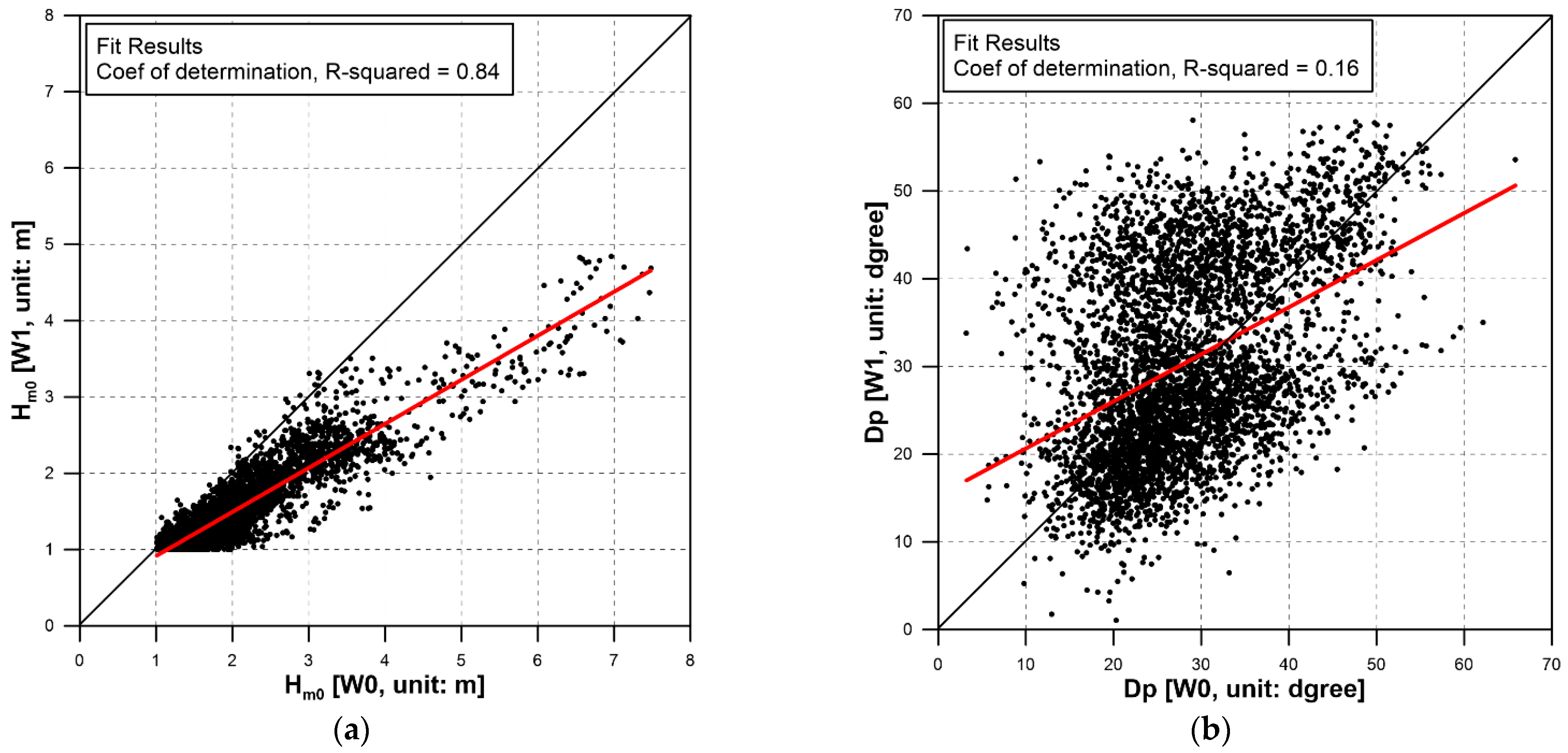
In Figure 7, $H_{m0}$ and $D_p$ are compared between the measurements at the two stations, W0 and W1. It is noted that the waves were not measured in W0 during BC01 (2008–2009), meaning that Figure 7 only compares the data at BC02 (2018–2019) and AC. In the case of $H_{m0}$, the data between the two locations show relatively high correlation with an $r^2$, the coefficient of determination, of 0.84. However, the $r^2$ for $D_p$ was as low as 0.16 between W0 and W1, which indicates that the directions of the waves that approached Yeongil Bay were not correlated with those that approached the detached breakwater. Therefore, to carry out a detailed investigation, it was necessary to examine the impact of wave direction based on the data in W1, as proposed in Section 1, in addition to the analysis based on the data in W0, which was conducted in [17]. In the present study, therefore, the data in W1 were considered the primary wave measurements outside Pohang New Port.

The correlation between the wave parameters inside and outside Pohang New Port was examined by defining a new parameter, the wave height reduction rate ($R_{W\#}$). $R_{W\#}$ was calculated from the ratio of $H_{m0}$ measured inside and outside the port (i.e., $R_{W2}=H_{m0}\left[W2\right]/H_{m0}\left[W1\right]$ and $R_{W3}=H_{m0}\left[W3\right]/H_{m0}\left[W1\right]$, etc.). 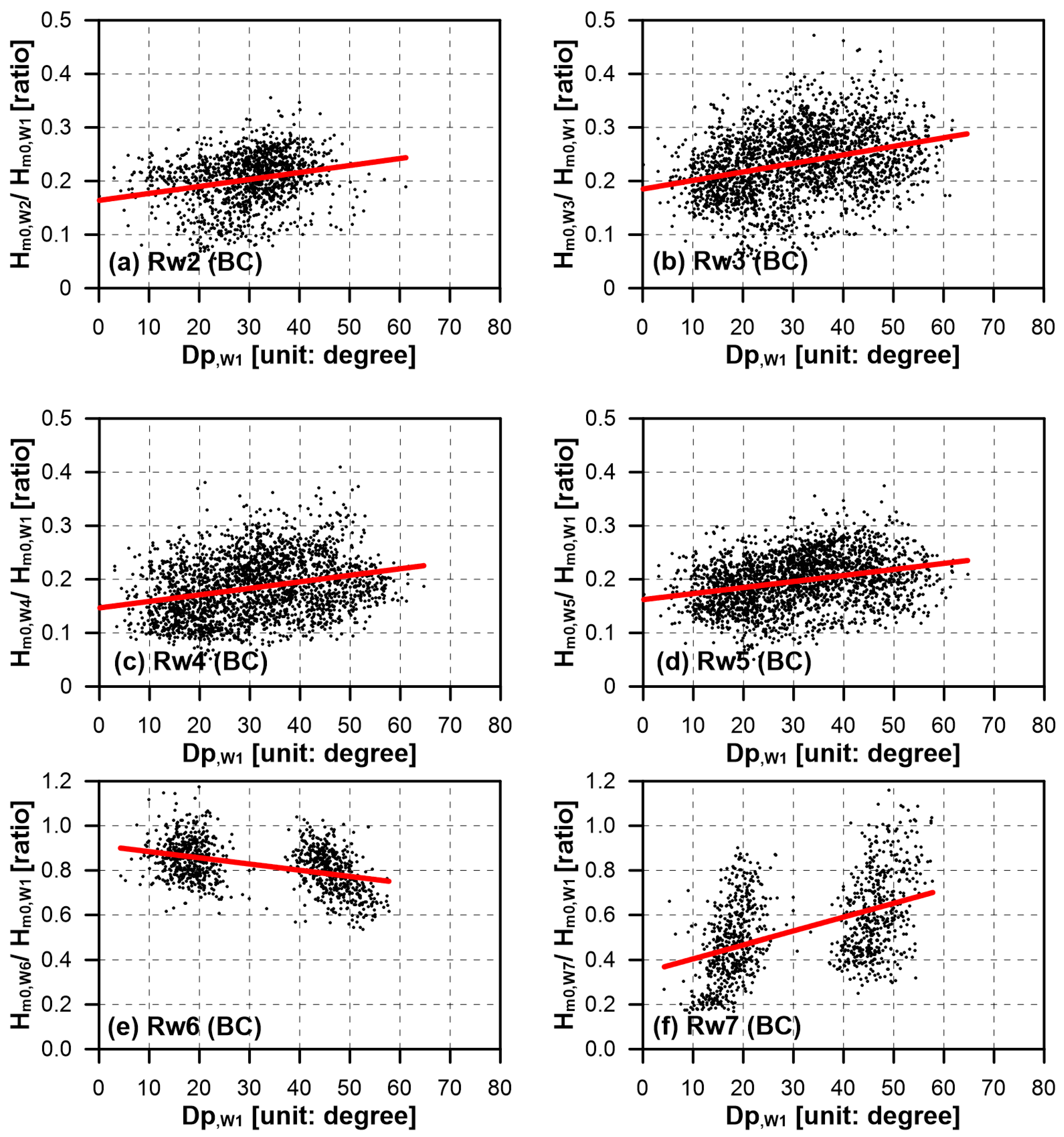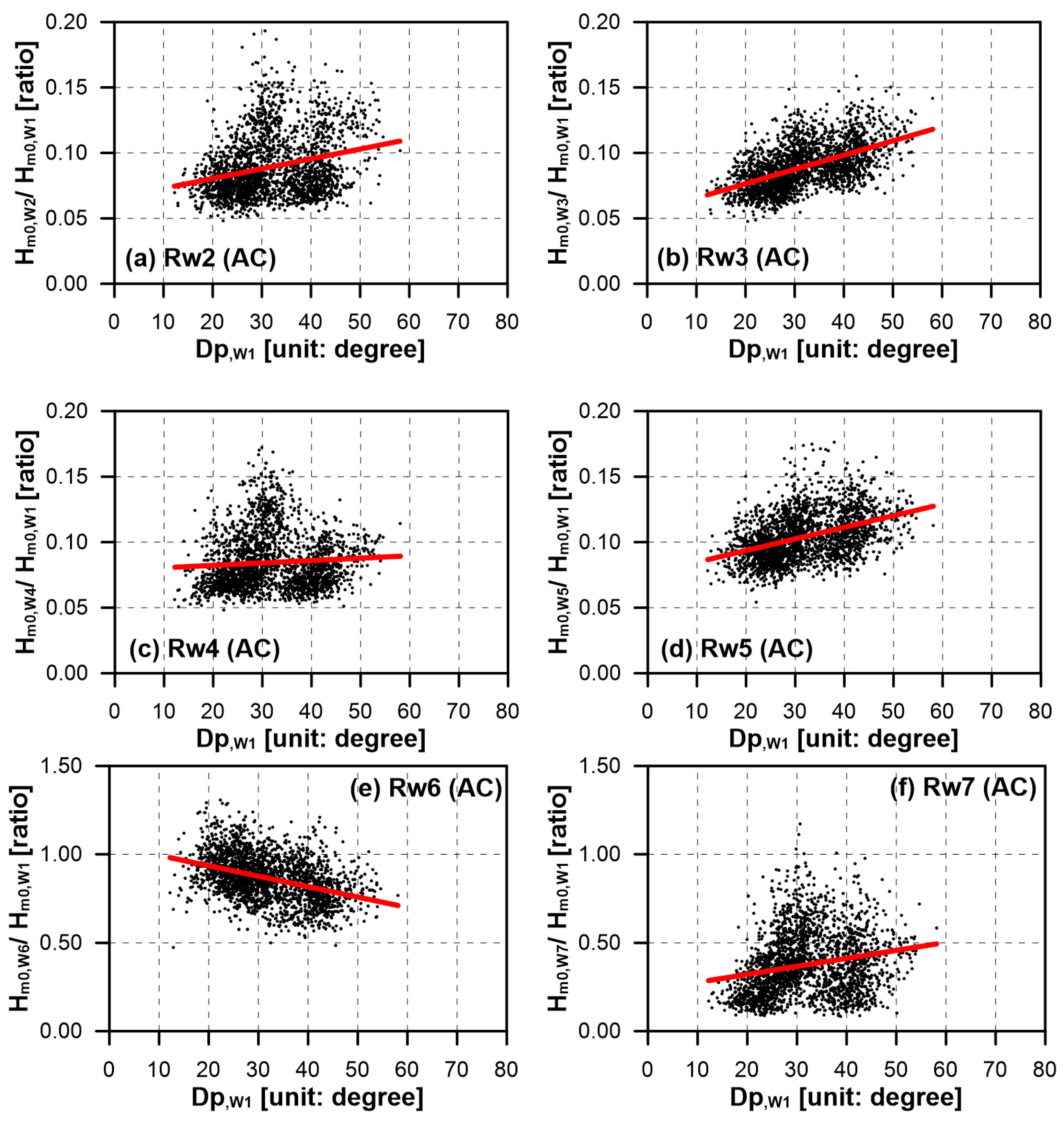The $R_{W\#}$ parameters were estimated from the data sets of 38 and 27 wave events selected for BC and AC, respectively, as described in Section 2.2, because the relationship between $R_{W\#}$ and $D_p$ was not clearly observed for waves with low energy. In Figure 8 and Figure 9, the distributions of $R_{W\#}$ versus $D_p$ in W1 for the data selected for the wave events are compared between BC and AC. In addition to the four stations inside the port, the $R_{W6}$ and $R_{W7}$ values were estimated outside the port as well. 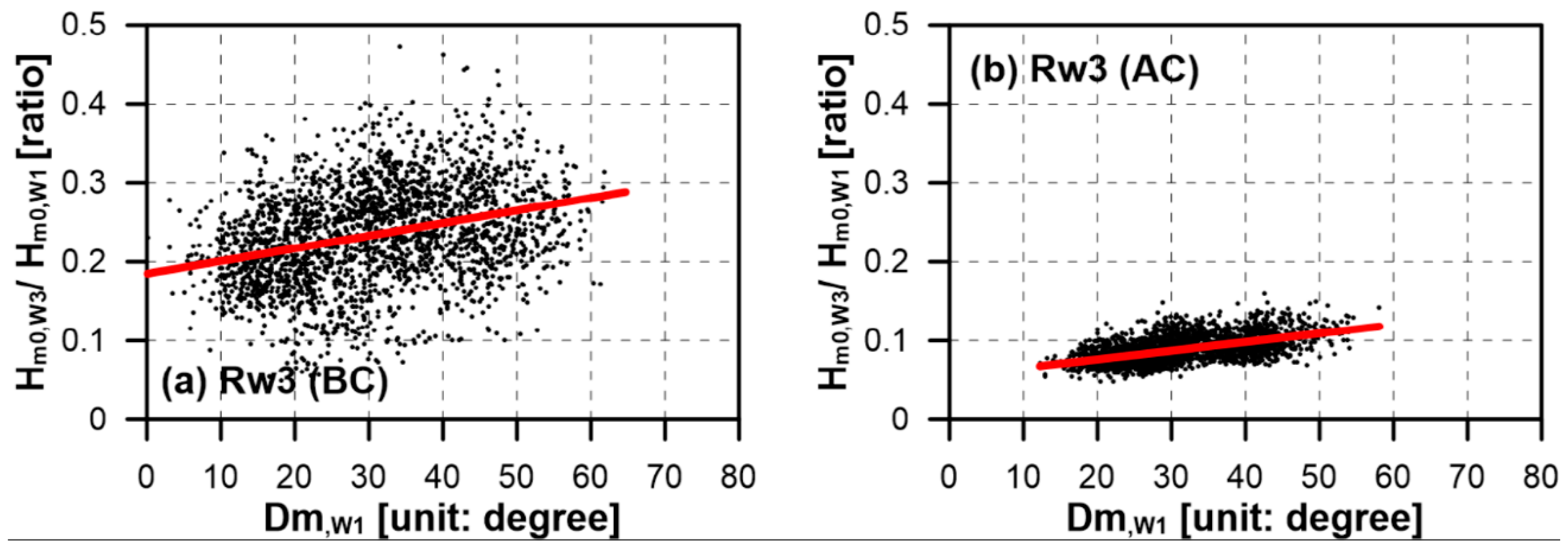Considering that the wave energy inside the port decreased with the decreasing magnitude of $R_{W\#}$, the results in Figure 8 and Figure 9 clearly show that the wave energy was much reduced in AC compared to that in BC, confirming the effectiveness of the detached breakwater in reducing the wave energy inside the port. 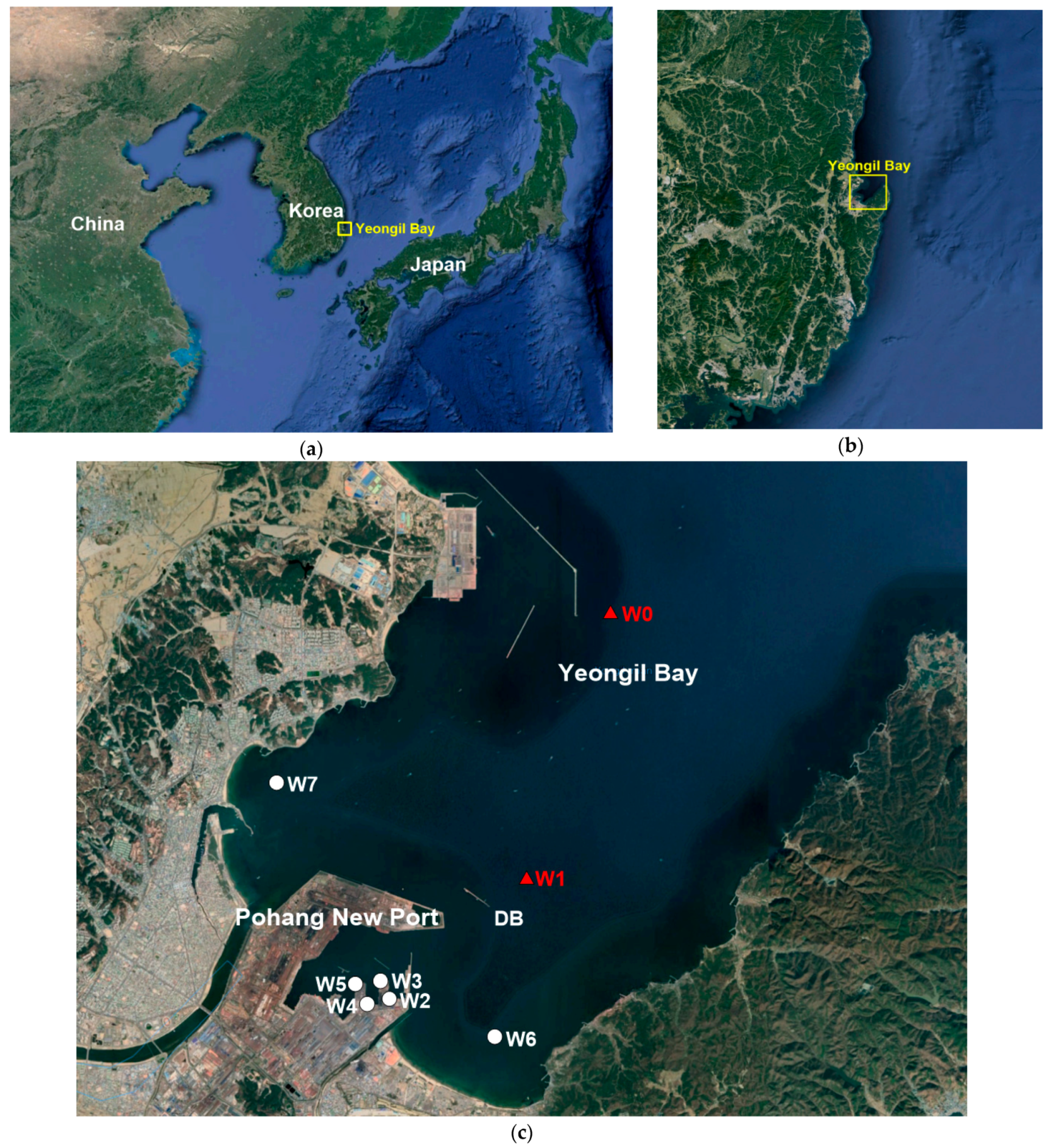It is also interesting to see that the $R_{W\#}$ value measured inside the port ($R_{W2}-R_{W5}$) tended to increase with $D_p$, showing that the $R_{W\#}$ value increased as the wave direction in W1 changed from N to NE. In contrast, the opposite phenomenon occurred in W6, the station in front of Dogu Beach outside the port (Figure 1c), at which the $R_{W6}$ value decreased with increasing $D_p$. On the other hand, the pattern in W7, the station in front of Yeongildae Beach, became similar to that inside the port, as the $R_{W7}$ value also increased with increasing $D_p$. The difference in the pattern of $R_{W\#}$ with $D_p$ in W6 and W7 might have been induced by their locations, which is discussed in Section 4. The correlation between $R_{W\#}$ and $D_p$ in BC was repeated in AC. However, the magnitude of $R_{W\#}$ measured inside the port was much lower in AC than that in BC, as its values in AC were ~50% of those in BC, which is discussed in Section 4. In Figure 8 and Figure 9, the red lines show linear regressions and the regression coefficients are listed in

Table 3. List of coefficients of determination ($r^2$) and linear regression coefficients (slope and intercept) for the scatter plots in Figure 8, Figure 9, Figure 10 and Figure 11.

Figure 8	(a)	(b)	(c)	(d)	(e)	(f)
$r^2$	0.055	0.097	0.072	0.084	0.172	0.225
Linear regression	0.0013X + 0.1638	0.0016X + 0.1850	0.0012X + 0.1468	0.0011X + 0.1621	−0.0028X + 0.9121	0.0062X + 0.3428
Figure 9	(a)	(b)	(c)	(d)	(e)	(f)
$r^2$	0.072	0.296	0.005	0.168	0.149	0.047
Linear regression	0.0008X + 0.0654	0.0011X + 0.0546	0.0002X + 0.0787	0.0009X + 0.0760	−0.0059X + 1.0529	0.0045X + 0.2308
Figure 10	(a)	(b)	(C)	(d)	(e)	(f)
$r^2$	0.035	0.000	0.000	0.014	0.011	0.000
Linear regression	−0.0212X + 0.2364	−0.0031X + 0.2388	−1.2018X + 0.1810	−0.0142X+ 0.2184	0.0299X + 0.7804	0.0053X + 0.5318
Figure 11	(a)	(b)	(C)	(d)	(e)	(f)
$r^2$	0.104	0.032	0.016	0.011	0.002	0.034
Linear regression	0.0115X + 0.0690	0.0045X + 0.0813	0.0041X + 0.0772	0.0029X + 0.0991	0.0091X + 0.8489	0.0640X + 0.4936

.

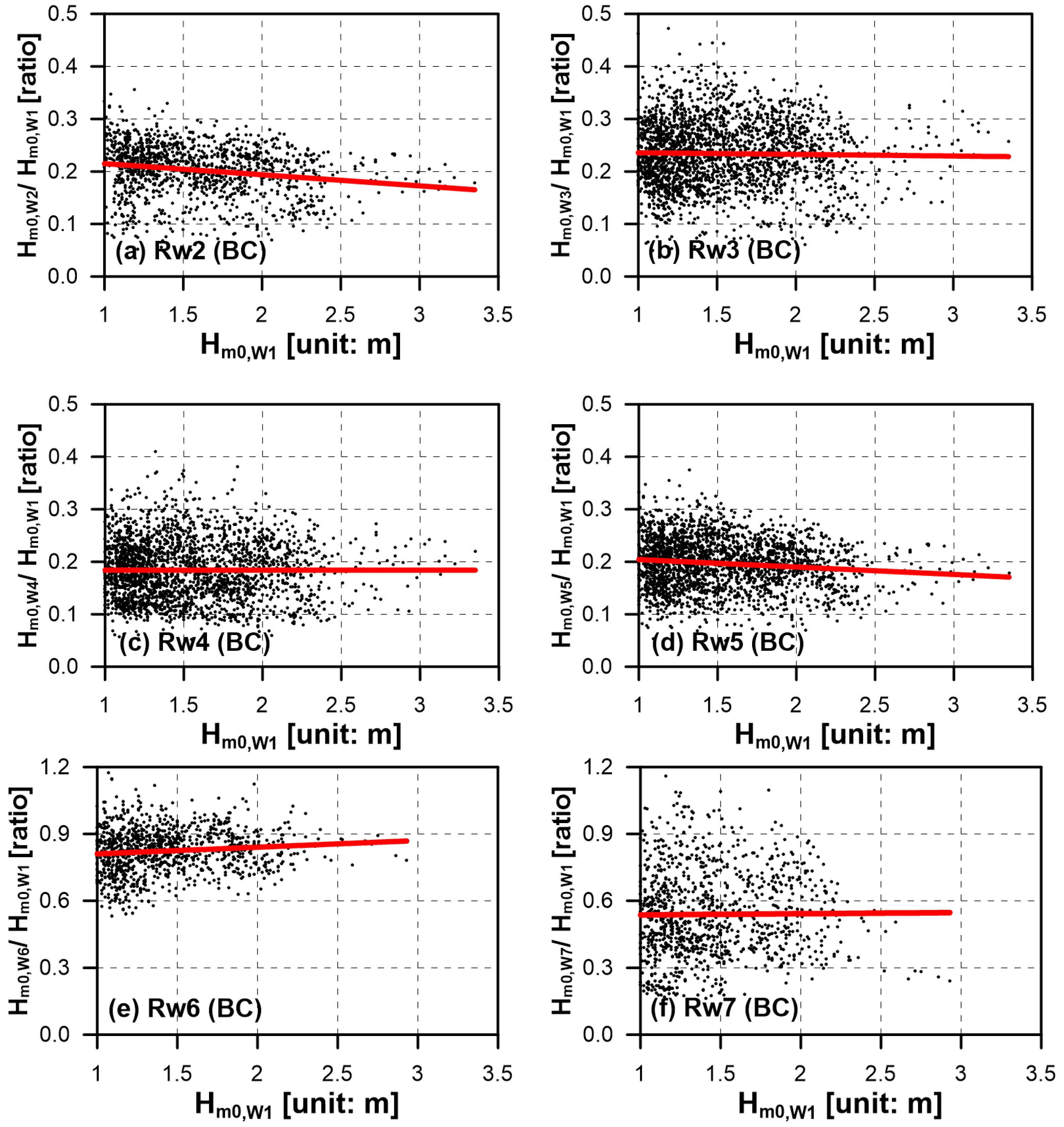
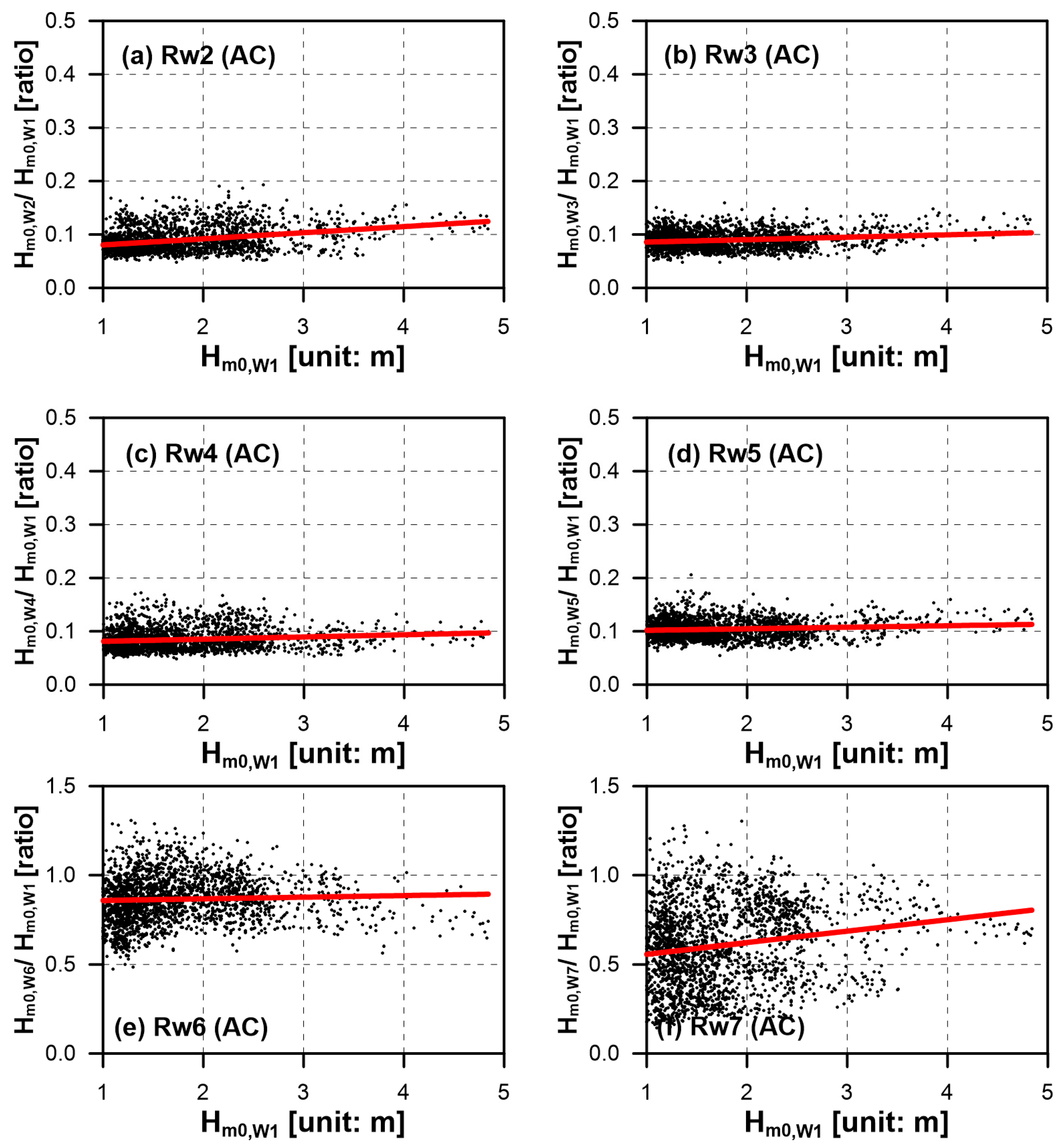
Considering that the $D_p$ value measured in W1 acted as a controlling factor on the wave reduction inside Pohang New Port, it was also necessary to examine the impact of the wave height on the wave reduction pattern. Figure 10 and Figure 11 show the scatter plots between $R_{W\#}$ and $H_{m0}$, measured in W1. It is observed that $R_{W\#}$ did not show a clear correlation with $H_{m0}$ in W1 for both BC and AC. It is noted that the time variation pattern of $H_{m0}$ measured inside the port was similar to that of $H_{m0}$ in W1, as shown in Figure 2 and Figure 5. Therefore, the low correlation between $R_{W\#}$ and $H_{m0}$ inside the port was an interesting result, indicating that the wave reduction process inside the port might not be dependent on the wave height, unlike the wave direction. The low correlation between $R_{W\#}$ and $H_{m0}$ was not only observed inside the port but also outside the port in W6 and W7 in both BC and AC. The results in this section are important, because the effect of the breakwater was confirmed, as not only the magnitude but also the variance in $R_{W\#}$ were significantly reduced in AC compared to those in BC, regardless of the wave height. In addition, the high dependence of the wave reduction process inside the port on the propagation direction of short waves outside the port required further analysis to understand the courses of wave propagation around the breakwater and the port, which was carried out using the BOUSS-2D model, which can simulate wave transformation around these complex structures, and the results are provided in the next section.

3.2. Numerical Model Results

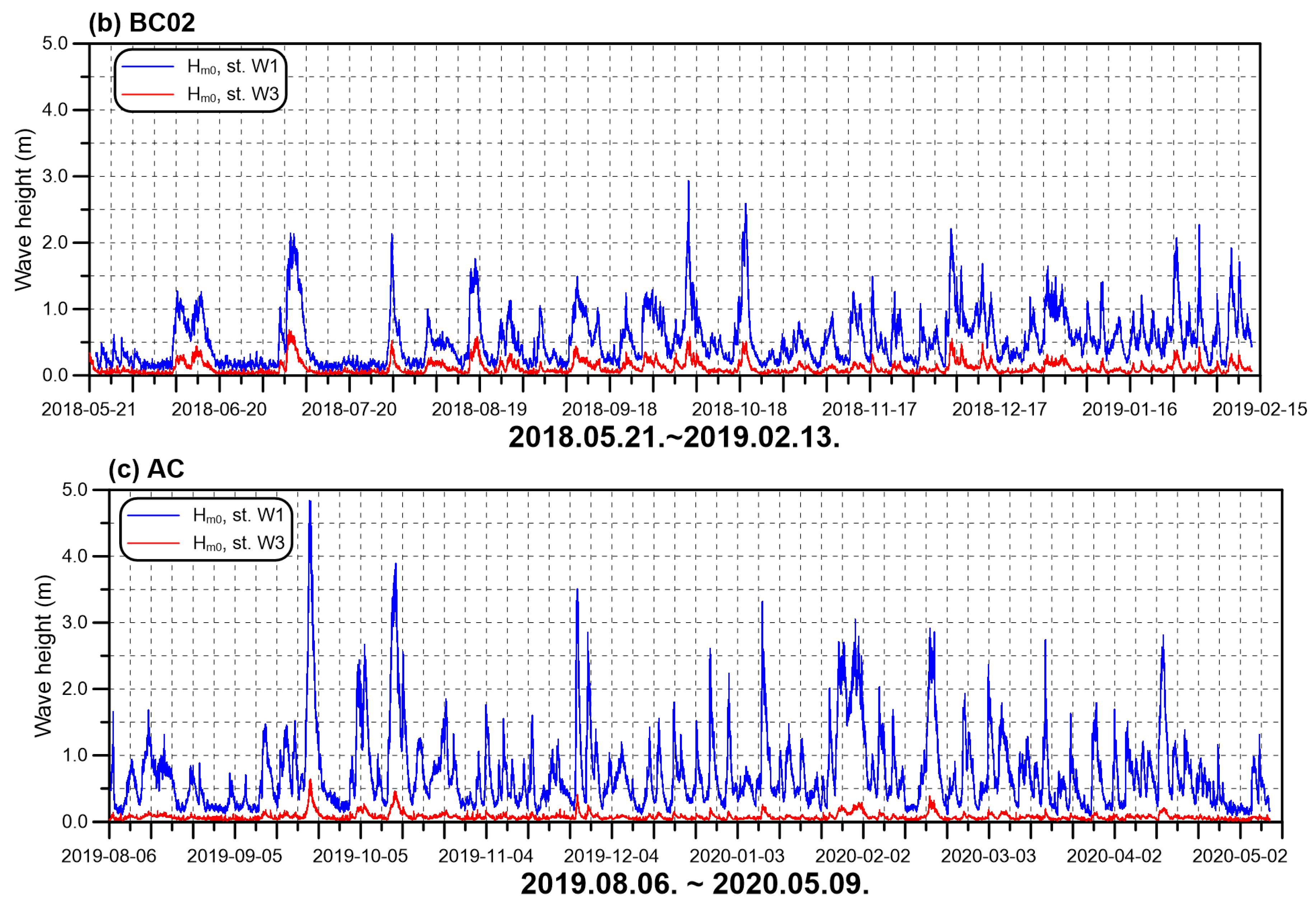
The BOUSS-2D wave model was set up as described in Section 2.3 for the two cases representing the wave propagation in BC and AC. The two cases were selected because they had the maximum wave heights during the period of the 38 (BC) and 27 (AC) wave events, as shown in Figure 3a,b. The events with the maximum $H_{m0}$ were selected because the effect of the detached breakwater in reducing the wave energy inside Pohang New Port could be more clearly observed under higher wave energy conditions.

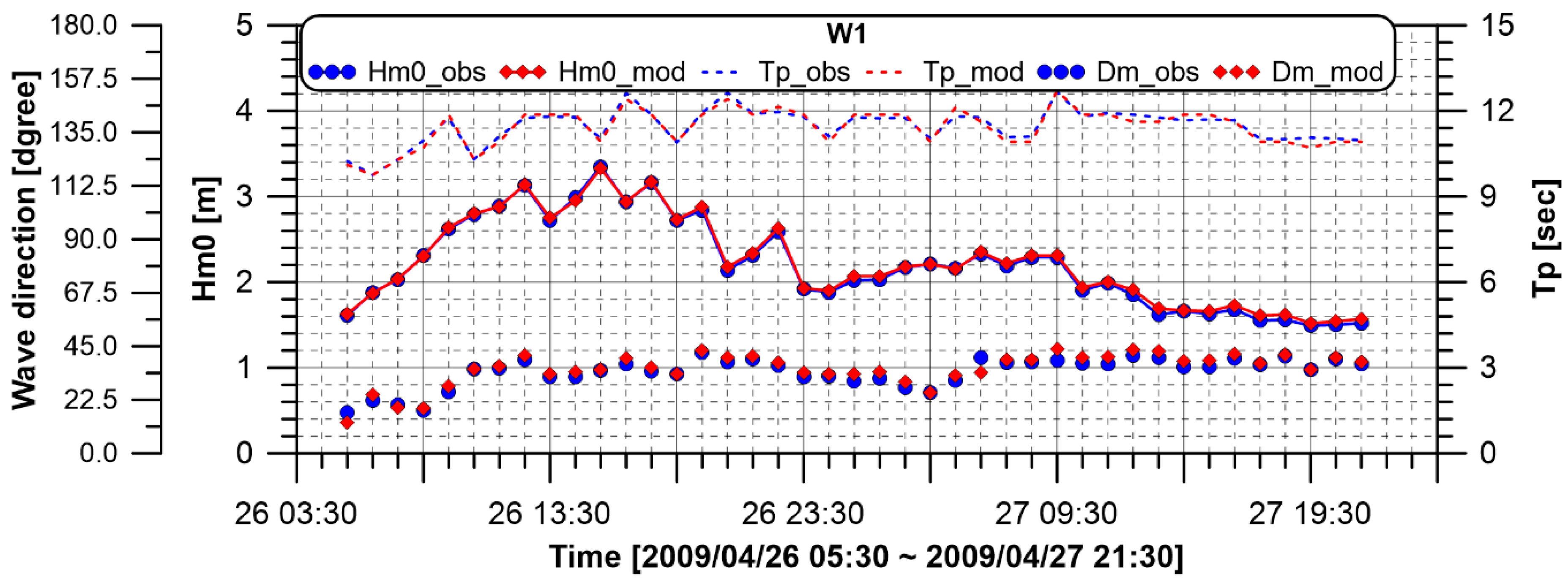
In Figure 12, the wave conditions in W1 are compared between the observed and modeled data from 26 to 27 April 2009, which were selected from the BC events. Considering the computational domain shown in Figure 4b, the location of W1 was close to the outside open boundary, and the modeled wave conditions were well matched with the observation data that were used for the boundary forcing conditions. The data show that the wave height increased to the maximum ($H_{m0}~$3.4 m) at 15:30 on 26 April 2009, and then, it gradually decreased. The wave period fluctuated between 9.2 and 12.2 s, and the $D_p$ value gradually increased from ~N12°E to ~N40°E, indicating that the waves were mainly approaching from NNE~NE in W1 during this wave event.

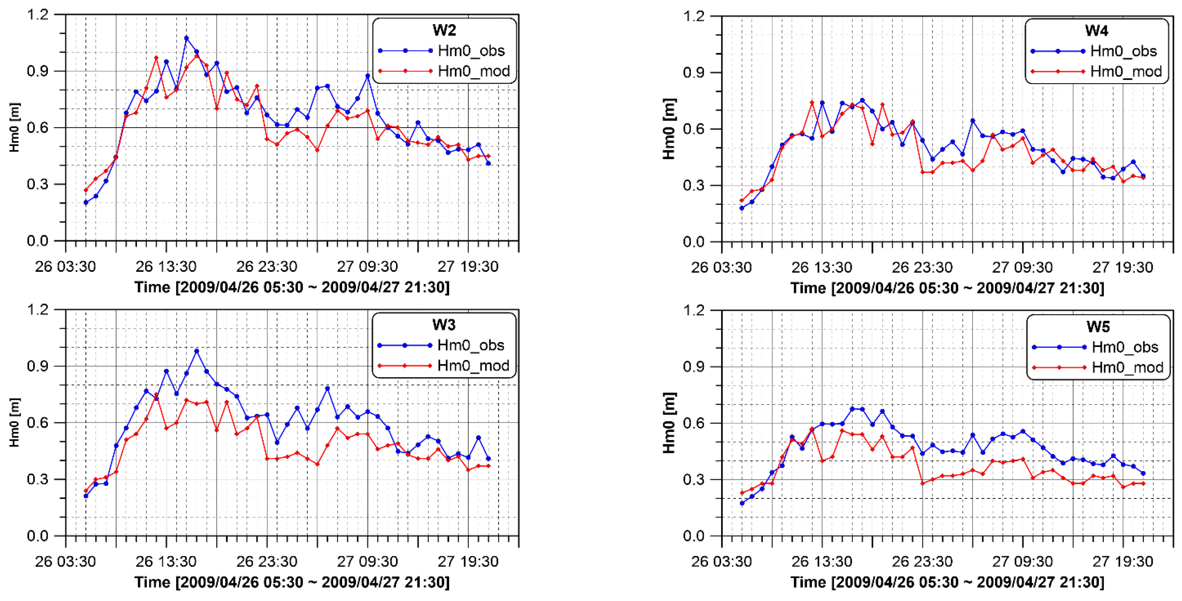
Figure 13 shows the comparisons of the modeled wave heights with observations at the four wave stations (W2, W3, W4, and W5) inside Pohang New Port to validate the model performance. Reasonable agreement was observed among the four wave stations inside the port (marked in Figure 4b), as the overall pattern of the $H_{m0}$ time variation generally agreed between the modeled and observation data, although the model results were underestimated, specifically in W3 and W5. The average error ($\frac{\sqrt{{\left(H_{obs}-H_{mod}\right)}^2}}{H_{obs}}\times 100$) was calculated, and it ranged from 12% to 23% (12.9%, 18.7%, 13.6%, and 22.7% for W2, W3, W4, and W5, respectively). It is noted that the errors were greater in the stations located outside the slits (W3 and W5) than those located inside the slits (W2 and W4). Although the reason for this is not yet clearly understood, the four wave stations were located in the corners of the slits where the incoming and reflected waves were interfered with in complicated ways, which could have increased the wave height compared to that in other areas near the slits and also could have increased the modeling errors. As the pattern of the $H_{m0}$ time variation of the model generally agreed with that shown in the observation, it could be concluded that the model was validated for the wave event, and the model results were further analyzed to understand the wave propagation pattern inside the port.

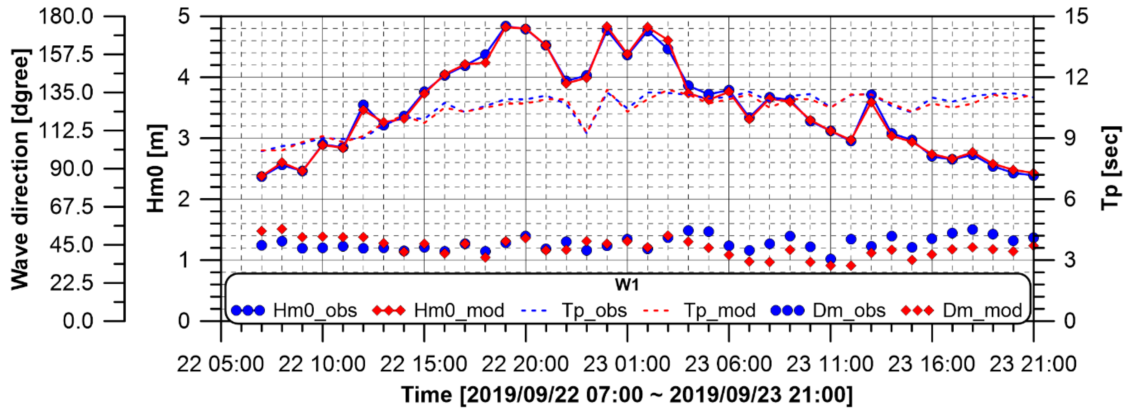
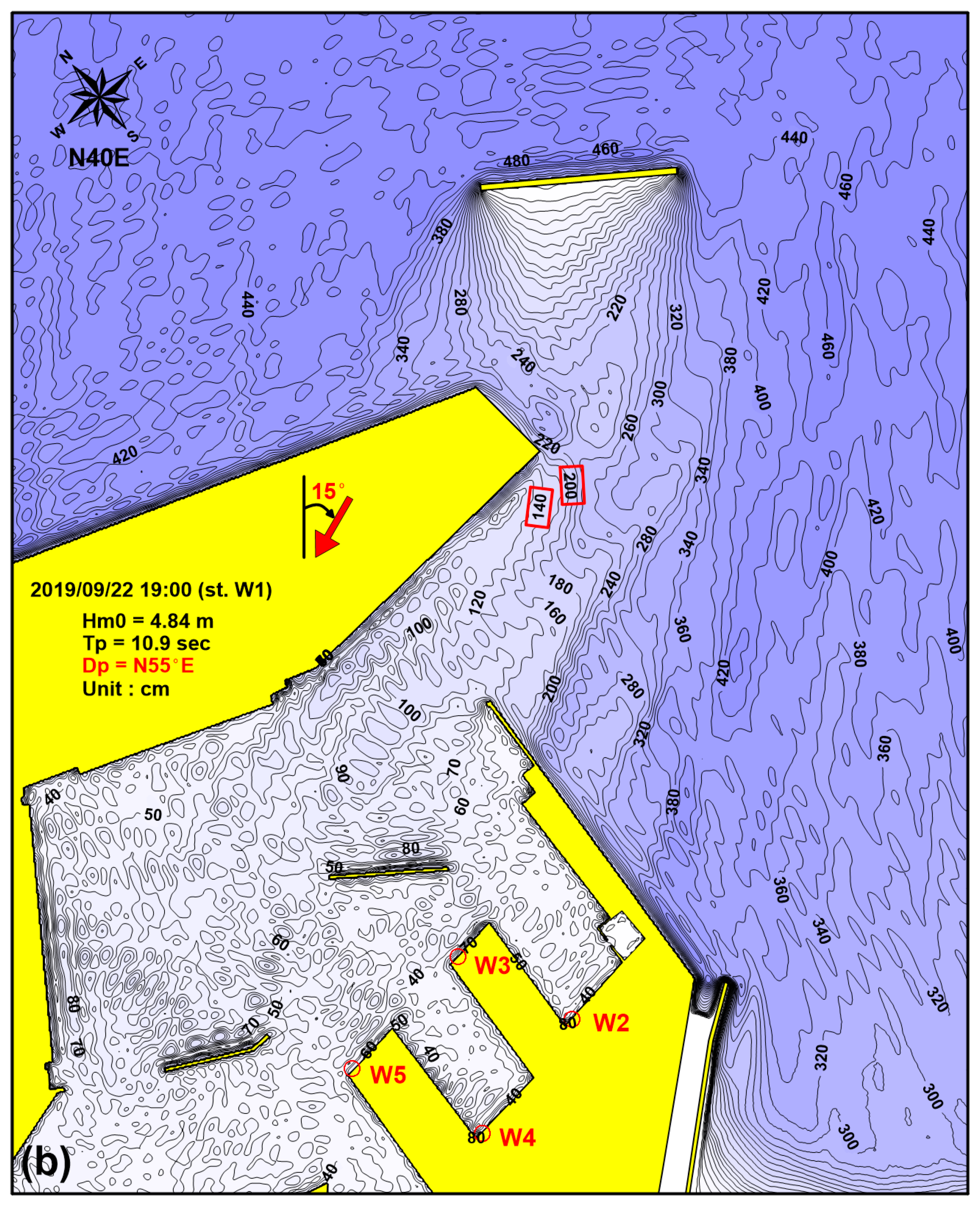
A similar comparison between the modeled and observational data was carried out for the selected event case in AC. In Figure 14, the observed and modeled wave conditions in W1 are plotted for the period of the wave event selected for AC, from 07:00 on the 22 to 21:00 on 23 September 2019. Similar to the event case in BC, the wave conditions in W1 were nicely matched between the model and observation due to the proximity of the location of W1 to the open boundary. It was shown that the wave height increased to become the maximum ($H_{m0}~4$.8 m) at 19:00 on 22 September 2019 and then gradually decreased to ~2.5 m at 21:00 on the 23rd in W1. The wave period generally increased from ~8.5 s to ~11.0 s, and the $D_p$ value fluctuated between 30$°$ and 60$°$, showing that the waves generally approached from NE in W1 during the wave event.

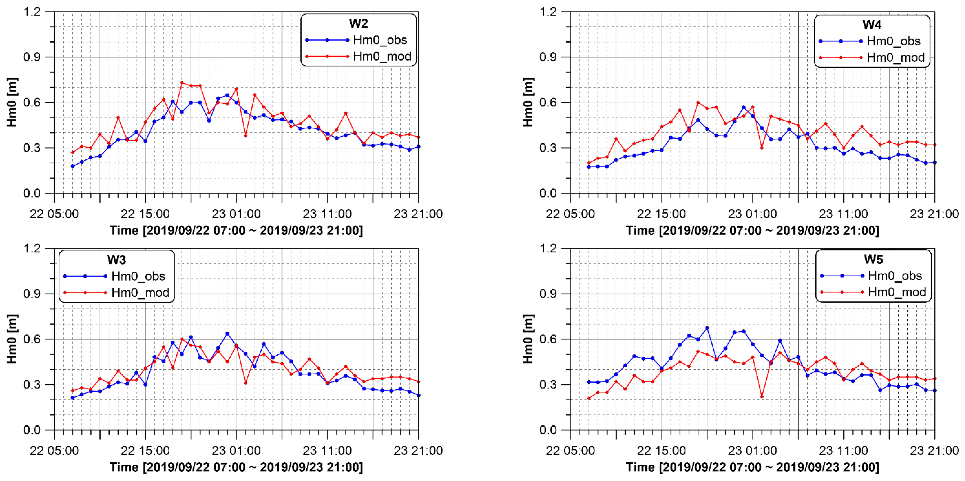
Figure 15 compares the modeled wave heights with the observed data at the four wave stations (W2, W3, W4, and W5) inside Pohang New Port during the wave event selected for AC. It shows that the pattern of wave height time variation during the event was successfully generated by the model, although the errors estimated from the wave height were not improved compared to those in BC, as they were ~19.2%, 17.1%, 31.3%, and 19.2% for W2, W3, W4, and W5 respectively. The higher error range in AC was likely due to the lower magnitude of the observed $H_{m0}$, which would increase the error for the same deviation between the model and observation data.

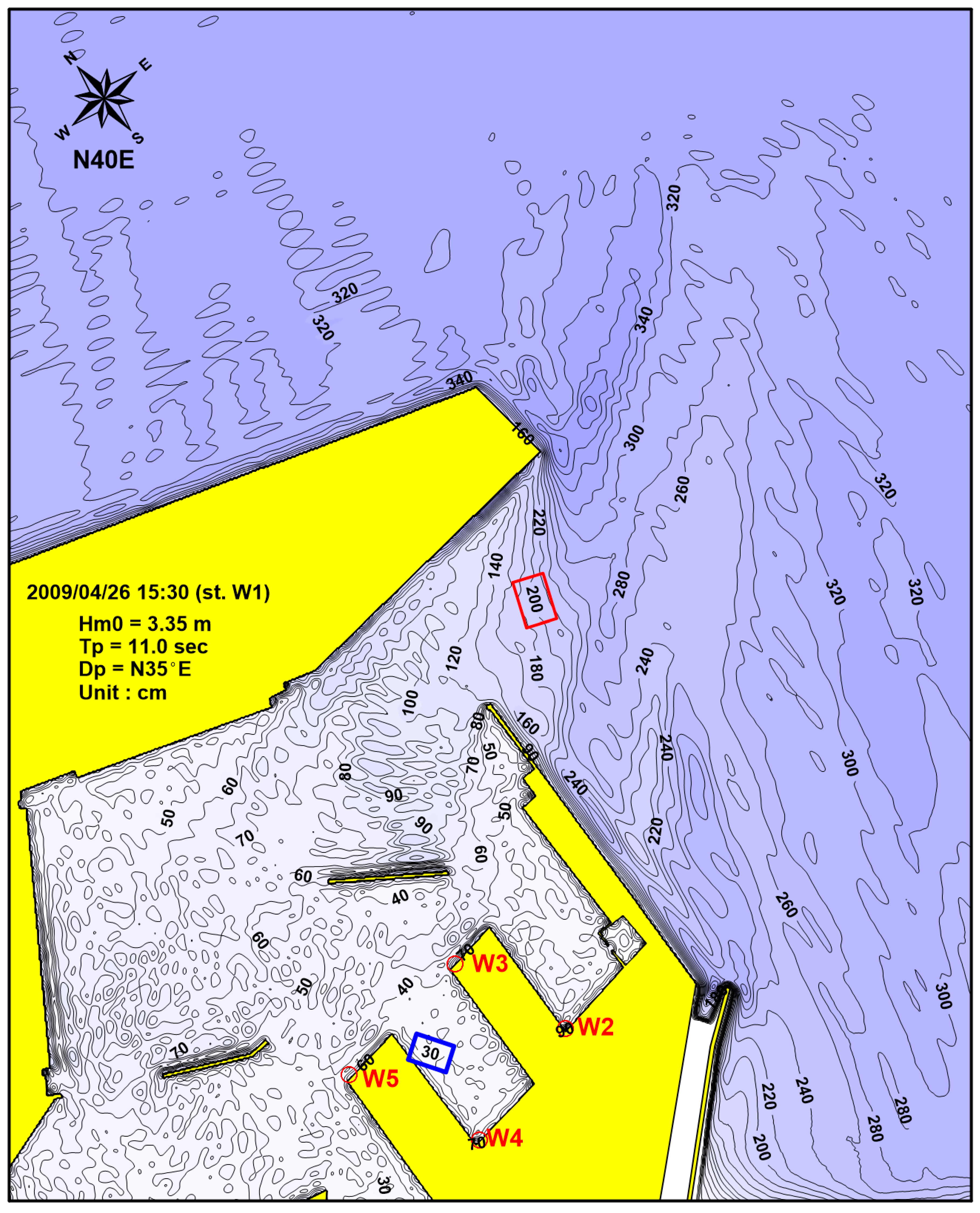
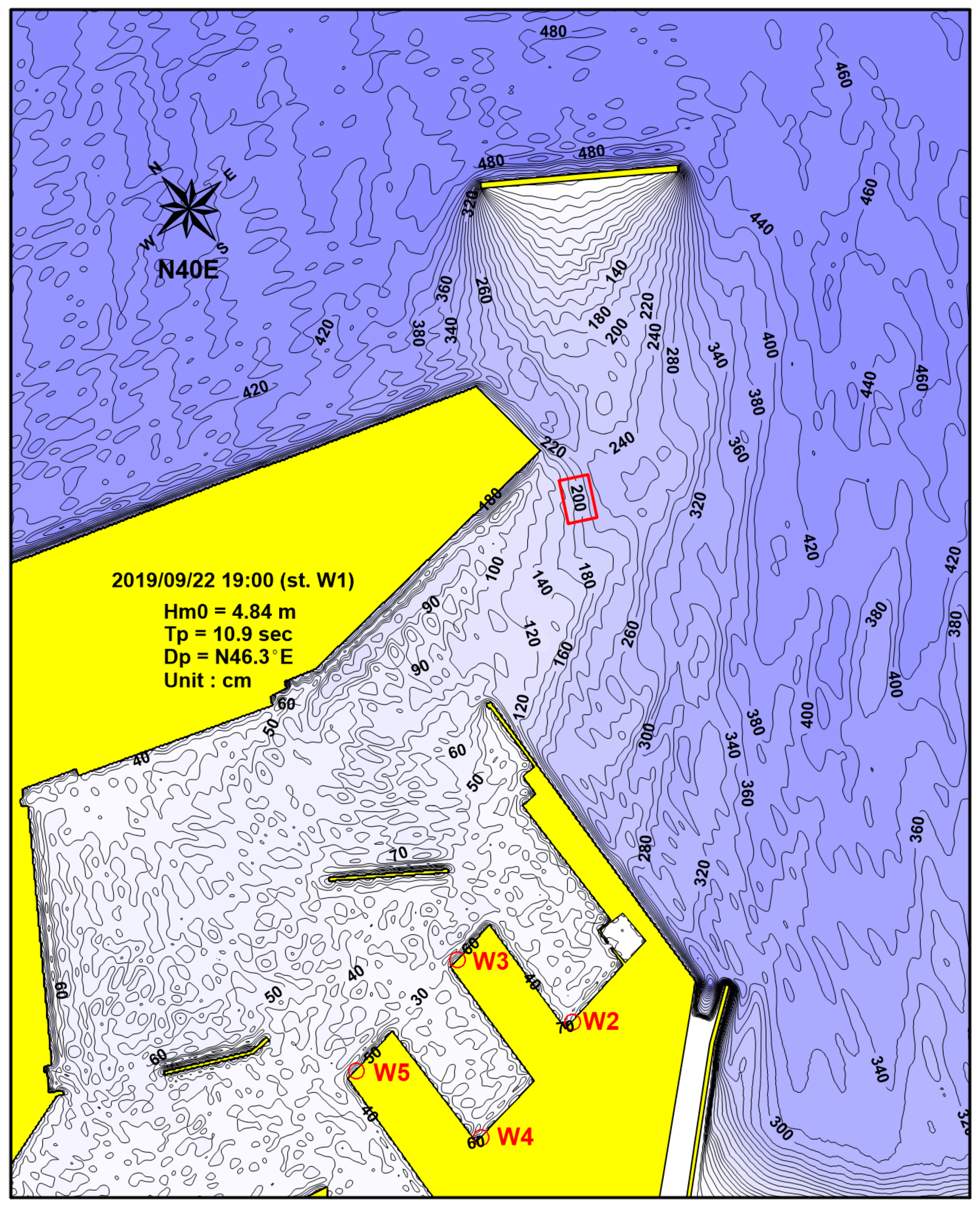
Once the BOUSS-2D model was validated, the next step was to analyze the course of wave propagation to understand how the wave energy was reduced inside Pohang New Port through a comparison between BC and AC. In Figure 16 and Figure 17, the contours of wave heights during the periods of the two wave events selected for BC and AC are compared. The contours are captured as a snapshot of the wave field at the time when the $H_{m0}$ value became the maximum for each event, as shown in Figure 12 and Figure 14. That is, in the case of BC, Figure 16 shows the field of wave heights at 15:30 on 26 April 2009 when the $H_{m0}$ value became the maximum, 3.35 m (Figure 14). Similarly, the wave height field is contoured in Figure 17 at 19:00 on 22 September 2019, as it is the time when the $H_{m0}$ value became the maximum (4.84 m) during the wave event selected for AC. The input wave conditions for the two cases were based on the observations at corresponding times. The wave period was similar between the two cases, as the $T_p$ value was 11.0 s and 10.9 s for BC and AC, respectively. The wave direction was N35.0°E for BC and N46.3°E for AC, as they were propagating in the NNE–NE directions. Along the open boundary that was rotated 40° in the NE direction (Figure 4a), the incident wave direction was nearly normal to the boundary in both BC and AC (with a deviation of 5°–6°), indicating there were no significant discrepancies in terms of the input wave propagation direction between the two cases.

Both of the figures effectively compare the pattern of wave reduction inside Pohang New Port between the two cases. In BC (Figure 16), the isolines of the wave height became parallel to the port entrance where the narrow navigation channel is connected to the inside of the port. At the port entrance, the $H_{m0}$ value was ~2.0 m (marked in a red rectangle in Figure 16), indicating that the $H_{m0}$ value was reduced by ~40% from the input wave height at the outer open boundary (3.35 m). Once the waves entered the port, the wave height was rapidly reduced due to the combined effects of refraction and diffraction around the slits and other harbor structures, with $H_{m0}$ varying from ~2.0 m to ~0.3 m. The wave height was observed to be 0.3 m inside the slit where the wave stations W4 and W5 were located (marked in a blue rectangle). It is noted, however, that the $H_{m0}$ value was increased to 0.9 and 0.7 at the locations of wave stations W2 and W4, which was likely because the reflected waves were interfered with at the wall of the slits to increase the $H_{m0}$ value to higher than that calculated off the walls.

In Figure 17, the $H_{m0}$ isolines are contoured for the wave event selected for AC, which occurred at 19:00 on 22 September 2019. Compared to the case of BC, the detached breakwater was constructed near W1, blocking the waves. Behind the breakwater, therefore, $H_{m0}$ was rapidly reduced, and the reduction rate was greater than that in BC. For example, the $H_{m0}$ value became ~2.0 m near the entrance of Pohang New Port (marked in a red rectangle), and the reduction rate was 59% considering that the input wave height on the boundary was 4.84 m in AC, which was ~19% greater than that in BC. In addition, in AC (Figure 17), the red rectangle that marks the isoline position of $H_{m0}$ = 2.0 m is located ~0.2 km further offshore compared to that in BC (compare with Figure 16), indicating that the wave heights inside the port would become lower than those in BC, assuming that the pattern of $H_{m0}$ reduction inside the port would be same between the two cases, which was also confirmed from a comparison of the observed and modeled wave heights between BC and AC in W2, W3, W4, and W5, as shown in Figure 13 and Figure 15.

Figure 16 and Figure 17 show the model that simulated the wave propagation patterns using the input conditions based on the observational data, and the input wave directions on the open boundary were similar between BC and AC, as they were N35.0°E and N46.3°E, respectively. 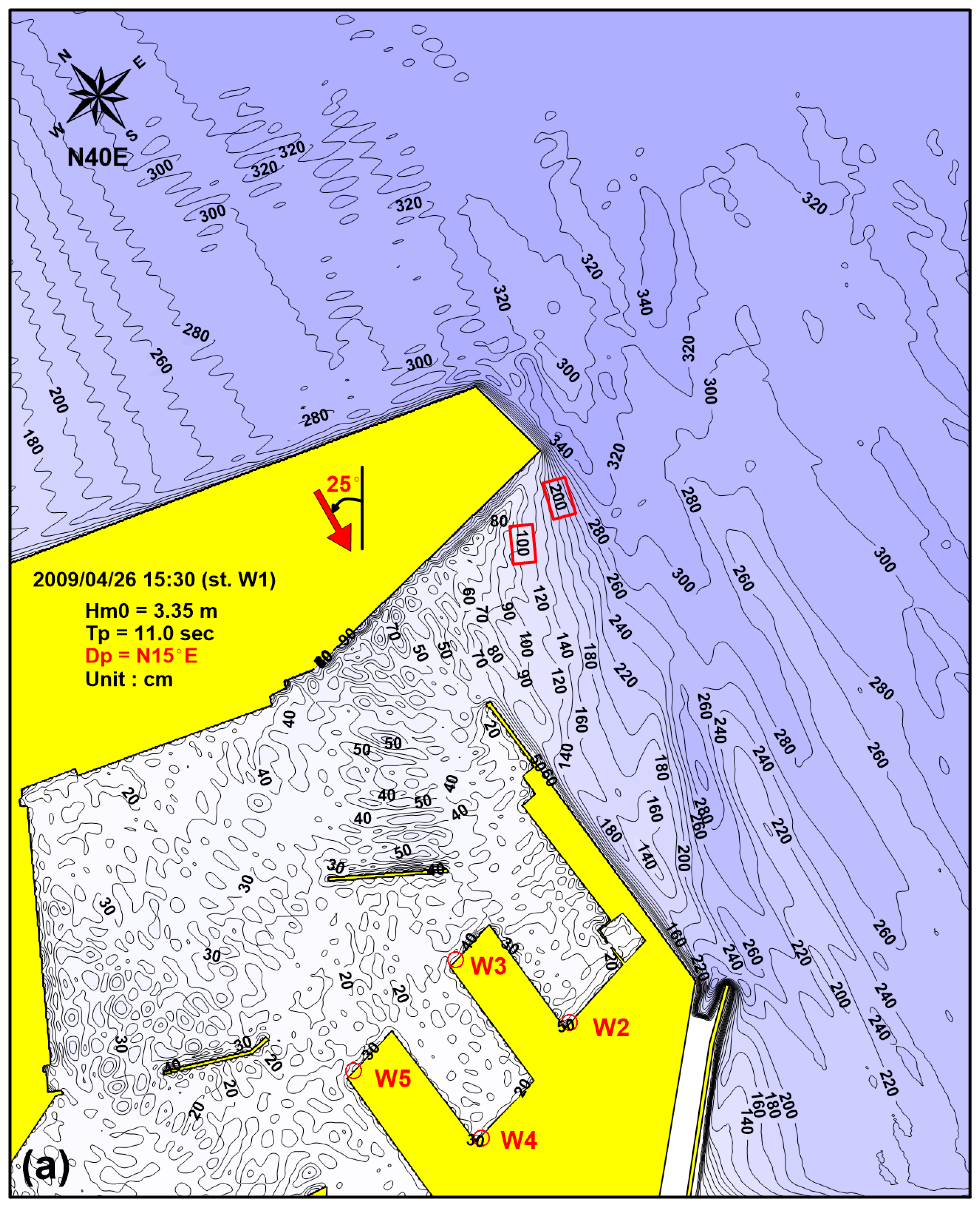Therefore, the impact of wave directional change on the wave pattern inside Pohang New Port could not be examined using these model results, although it was observed from the observational data, as shown in Figure 8 and Figure 9. In Figure 18, the two additional cases that were tested for BC by assuming extreme cases in the wave propagation direction are shown. It is noted that most of the measured $D_p$ values in W1 ranged between N15.0°E and N55.0°E in the case of AC, as shown in Figure 9. In Figure 18, therefore, the results of two model runs are shown with $D_p$ set as N15.0°E (Figure 18a) and N55.0°E (Figure 18b), as they represent the extreme wave directions for NNE and NE waves, respectively. Except for the wave direction, the other input wave conditions were the same as those given for the case of BC in Figure 16. The results of these two extreme cases in Figure 18 could help us to understand the different patterns in the wave energy reduction rate inside Pohang New Port, according to the changes in $D_p$ in W1, as observed in Figure 8 in the case of BC. In the extreme NNE case ($D_p$ = N15.0°E), the propagating waves outside the port mainly passed by the entrance of the port, and only the diffracted waves could enter the port, which increased the wave height reduction near the port entrance (Figure 18a). For example, the $H_{m0}$ value was as high as 2.0 m just outside the port entrance, but it was reduced to 1.0 m just inside the port, as the distance between the two positions was only ~0.5 km (marked with two red rectangles). 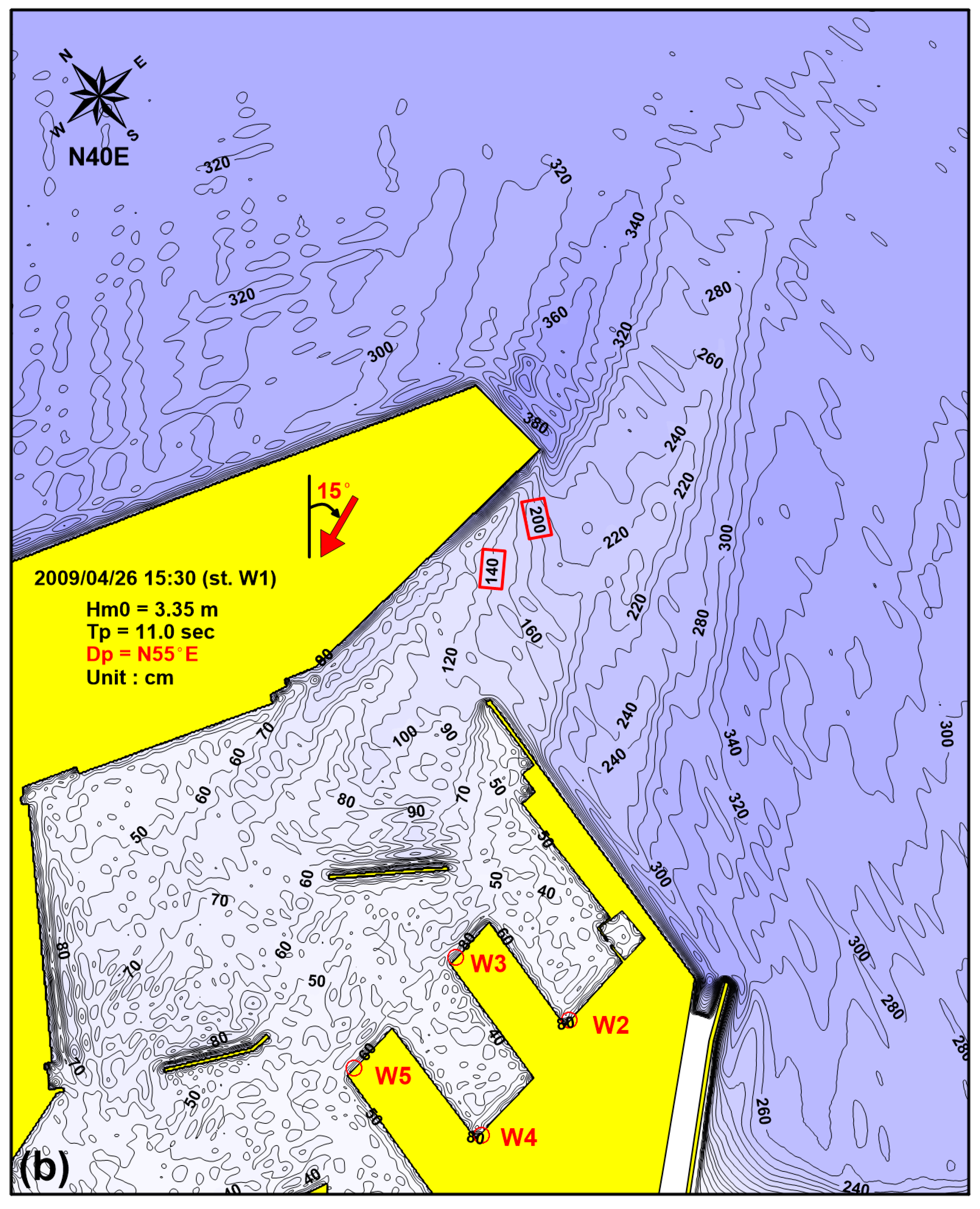The high wave reduction rate near the port entrance meant that $H_{m0}$ ranged from 0.2 to 0.7 m inside the port, and the estimated wave height reduction rate ($R_{W\left(model\right)}=\frac{H_{m0}\left[inside PNP\right]}{H_{m0}\left[\mathrm{open} \mathrm{boundary}\right]}$) was 5–20%. On the contrary, in the extreme NE case ($D_p$ = N55.0°E) shown in Figure 18b, the wave reduction near the port entrance was less severe compared to that in Figure 18a, as shown in the two marked red rectangles (the $H_{m0}$ value was reduced from 2.0 m to 1.4 m for ~0.5 km). Therefore, the $H_{m0}$ value inside the port was also higher compared to those in Figure 18a, with a range of 0.4–1.2 m in the areas, providing $R_{W\left(model\right)}$ = 12–35% inside the port.

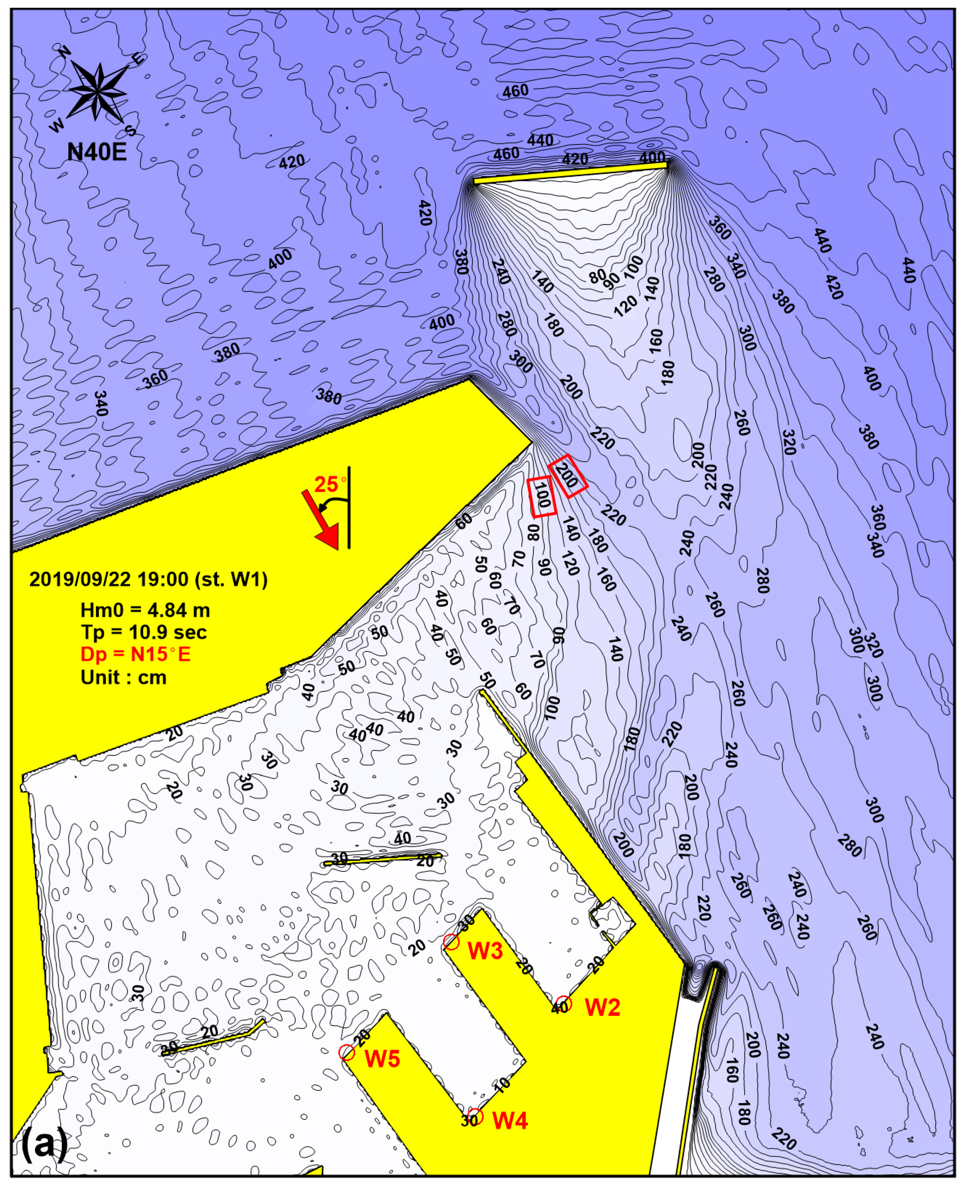
Figure 19 shows the model results of the two extreme wave directions that were tested for AC as well. That is, the other wave conditions were identical to those used in Figure 17, except that $D_p$ was set as N15.0°E (N55.0°E), which represented an example of extreme conditions of NNE (NE) waves, as shown in Figure 19a (Figure 19b). Similar to the cases in BC, the wave propagation pattern inside Pohang New Port was affected by the different $D_p$ input conditions at the open boundary, regardless of the existence of the detached breakwater. When $D_p$ was N15.0°E, the $H_{m0}$ value was significantly reduced in the lee area of the breakwater, as it was ~4.6 m offshore of the breakwater but decreased to ~2.0 m just outside the port, as shown in Figure 19a (marked with a red rectangle). The waves were then diffracted near the entrance of the port, where strong $H_{m0}$ reduction occurred for the waves entering the port, as the $H_{m0}$ value was reduced to ~1.0 m just inside the port (marked with a red rectangle). The range of $H_{m0}$ was then 0.2–0.7 m inside the port, leading to $R_{W\left(model\right)}$ = 5–15% inside the port. In the case of extreme NE waves ($D_p$ = N55.0°E in Figure 19b), the waves approached the port from the NE direction, meaning the detached breakwater became less effective in reducing the wave height. For example, the $H_{m0}$ value was reduced from ~2.0 m to ~1.4 m (marked in the red rectangles in Figure 19b) for the similar distance marked in Figure 19a. As a result, the $H_{m0}$ value became higher inside the port, compared to that of $D_p$ with N15.0°E, with the $H_{m0}$ range of 0.4–1.2 m inside the port, providing $R_{W\left(model\right)}$ of 8–25% (Figure 19b). The impact of wave direction in the case of AC is further discussed in Section 4.

4. Discussion

One of the most significant results of the present study was that the wave height reduction inside Pohang New Port was affected by the propagating wave directions that approached the detached breakwater. For example, in all of the wave stations inside the port, $R_{W\#}$ increased with increasing $D_p$. The close correlation between $R_{W\#}$ was observed in both BC and AC, as shown in Figure 8 and Figure 9. However, the magnitude of $R_{W\#}$ became lower in AC. Figure 20 shows the comparison of the scatter plots of $R_{W3}$ in terms of $D_p$ between BC and AC. The distribution of the wave reduction rate was compared in W3 because it was located closest to the entrance of the port; thus, the impact of the wave propagation direction could be distinct in this station. The figure shows that $R_{W3}$ increased with an increasing $D_p$ value in both BC and AC. However, the magnitude of $R_{W3}$ ranged from 0.12 to 0.40 in BC, but the magnitude was reduced by ~40% in AC, as $R_{W3}$ ranged from 0.05 to 0.15. The lower magnitude of $R_{W3}$ in AC indicates that the wave energy was effectively reduced inside the port, confirming the effect of the detached breakwater in securing the tranquility of the port.

Regardless of the observation of the significantly lower values of $R_{W\#}$ in AC, the result in Figure 20b indicates that the reduction in the wave height inside Pohang New Port became less effective even with the protection provided by the detached breakwater if the wave propagation direction increased (i.e., changed from NNE to NE). The cause for this was investigated using the BOUSS-2D model, which is displayed in Figure 19, showing that the wave heights were higher in the lee of the breakwater and also in the areas near the port entrance, as well as inside the port when the waves approached in the extreme NE direction (N55°E), which raised a question—“is the construction of a detached breakwater, as shown in Figure 1c, sufficient to reduce the wave energy in securing the tranquility inside the port for the waves approaching in all directions?” To find the answer, we needed to account for the fact that the eastern end of the breakwater was located near the western end of the navigation channel (see Figure 4b). From the engineering aspect, therefore, it was not practical to extend the breakwater further to the SE because the detached breakwater would then block the navigation channel. An alternative option would be to place another detached breakwater further SE, avoiding the navigation channel. However, this second option would not be effective either, considering that the extreme NE waves would approach in the N55.0°E direction, and thus, the new detached breakwater may be useless in blocking the waves propagating to the port entrance. Therefore, alternative options to construct additional engineering measures may not be practical, unless unavoidable.

The next step to find an answer to the question would be a statistical approach. From the results in Figure 9, it was shown that the magnitude of $R_{W\#}$ of the waves with $D_p$ values greater than N55°E was mostly not higher than 0.15 at the wave stations located inside the port (W2–W5). In addition, as described in Section 1, the targeted maximum wave height to maintain the desired harbor tranquility inside the port was proposed as 0.3 m [13]. Therefore, considering that the maximum $R_{W\#}$ of the waves with $D_p$ values greater than N55°E would be 0.15 for AC, the maximum $H_{m0}$ value in W1 that would enable the tranquility inside the port to be maintained can be calculated as 0.3/0.15 = 2.0 m. Based on the wave measurements in W1 during the whole period of AC, in total, there was only 1 h in which the observed waves had $D_p$ values greater than N55°E and $H_{m0}$ values greater than 2 m. As this number is too small compared to the total period of wave measurement of 278 days in AC, the criteria for the extreme NE direction could be extended to N50°E and even to N45°E. In these cases, however, the time in which the $D_p$ value was greater than N55°E and the $H_{m0}$ value was greater than 2 m was only 11 and 33 h, respectively, indicating that the probability of waves with heights that could be greater than 0.3 m inside the port because they approached from the extreme NE directions was ~0.0% (>N55°E), and it would only become 0.2% (>N50°E) and 0.5% (>N55°E) if the criteria for the extreme NE direction were extended. Therefore, it can be concluded that the detached breakwater located in the current position was sufficient to protect the port by maintaining its tranquility with the targeted wave height, and no further secondary engineering structures would then be required. This recommendation provided to elevate the effectiveness of the detached breakwater could be determined based on the amount of observational data measured in both periods in BC and AC. Without these wave measurements, the model results could lead to overestimation or underestimation in evaluating the effect of the breakwater. Although this result was only found in this specific case, it can also provide an insight for future studies in planning/operating ports under similar environments in which unexpected extreme cases should be carefully considered, and these extremes may need to be evaluated from the sufficient data sets observed in the field.

5. Conclusions

In this study, observational and numerical experiments were conducted to investigate the effect of the detached breakwater on reducing the wave energy inside Pohang New Port in terms of the wave parameters and specifically, the wave propagation direction. The reason for selecting the wave direction as a primary controlling factor was to examine whether the position of the detached breakwater was appropriate in reducing the wave energy inside the port for the waves that approached in all practical directions. If not, it may have been necessary to consider placing additional structure(s) to secure the tranquility inside the port. For this purpose, wave data were measured before (BC) and after (AC) the detached breakwater was constructed at multiple stations inside and outside the port. In addition, the BOUSS-2D model based on Boussinesq-type equations was employed to investigate the effect of the detached breakwater on the wave propagation pattern around the breakwater and inside the port.

The observational results show that the wave energy (the ratio of $H_{m0}$ inside and outside Pohang New Port) significantly decreased inside the port in AC compared to that in BC, although the wave height condition was generally higher outside the port (near the detached breakwater) in AC, which confirmed the effect of the breakwater. The reduction in the wave energy was observed in all wave propagation directions measured outside the port; however, the reduction rates inside the port showed that the effectiveness of the breakwater decreased as the wave direction changed from NNE to NE. The causes for the difference in the detached breakwater’s effect depending on wave directions were investigated based on the model results, which made it possible to investigate the wave propagation pattern around the breakwater. In the case of BC, the model results showed that more wave energy could be transferred inside the port without severe transformation when the waves approached in the NE direction, which could be difficult for the waves approaching in the NNE direction as the waves mostly passed by the entrance of the port. In the case of the AC model runs, the detached breakwater could effectively block the waves that approached in both the NNE and NE directions, resulting in significantly enhanced wave reduction rates inside the port. In the extreme case of NE waves (e.g., wave direction = N55.0°E) however, the wave energy increased inside the port regardless of the blocking caused by the breakwater, which might have required the consideration of additional engineering measures to secure the port tranquility. However, placing a secondary detached breakwater would not be practical because the location of the current breakwater is too close to the navigational channel, meaning that further extension of the existing detached breakwater could block the channel itself. Further investigation based on the observational data showed that the probability of the wave height inside the port exceeding 0.3 m (the target wave height to maintain the tranquility inside the port) was only 0.2–0.5% when the waves approached in the extreme NE direction, indicating that no secondary structures might be necessary and that the existing detached breakwater would be enough to secure tranquility inside Pohang New Port.