Extended State Observer-Based Fuzzy Adaptive Backstepping Force Control of a Deep-Sea Hydraulic Manipulator with Long Transmission Pipelines

Abstract

The force tracking control of deep-sea hydraulic manipulator systems with long transmission pipelines is disposed via fuzzy adaptive backstepping control based on an extended state observer in this paper. The pipeline model is established and then used to estimate the pressures in cylinder chambers, which are used to obtain the output force. In this process, the velocity of the piston, which is unmeasured, is needed, and an extended state observer is constructed to estimate the unmeasurable velocity signal. To cope with parameter uncertainties caused by changes in working depth, an adaptive algorithm is combined with the backstepping controller. Fuzzy logic is employed to design self-tuners that can automatically adjust the control parameters to guarantee force control performance from shallow seas to deep seas. The experimental results illustrate the success of the proposed control method. Comparative experimental results demonstrate that the extended state observer-based fuzzy adaptive backstepping controller has a relatively better tracking performance in different working conditions.

1. Introduction

Due to their large output force/torque, high power-to-weight ratio and overload protection, deep-sea hydraulic manipulators equipped on underwater vehicles, including Human-Occupied Vehicles and Remotely Operated Vehicles, have become essential tools for subsea tasks such as drilling, sampling, coring and connector mating in scientific research and ocean engineering [1,2]. A few commercial underwater hydraulic manipulators that are not equipped with position sensors are operated in the speed control mode, where the motion of joint actuators is controlled by proportional valves, and such a system belongs to open control systems [3]. Most underwater hydraulic manipulators are equipped with position sensors in each joint and are controlled in the position mode. Combined with the position information feedback from sensors, servo valves can realize closed-loop manipulator joint position control.

Marine archaeology and in situ experiments have become the focus of deep-sea scientific research in recent years [4,5]. To ensure the integrity of the samples and precise experimental operation, the interaction forces between deep-sea hydraulic manipulators and objects in complex deep-ocean environments actively need to be well controlled [6]. In some special environments, such as the deep-ocean environment, there are no high-precision force sensors that can be used on deep-sea hydraulic manipulators, and it is difficult to realize force feedback from force sensors. Deep-sea hydraulic manipulators with no tactile or contact sensing for monitoring or controlling the contact force can cause damage to themselves and objects. As typical joints of deep-sea hydraulic manipulators, if the output force tracking of hydraulic cylinders can be achieved, the force control of deep-sea hydraulic manipulators can hopefully be achieved.

A typical mainframe mechanical structure of deep-sea hydraulic manipulators consists of linear cylinders, a rotary actuator, a cycloid motor, etc. [7], as shown in Figure 1. The linear cylinders are key parts. There are currently no force sensors available for use in deep-sea environments. In this case, cylinder pressures can be used as feedback to realize the output force control of hydraulic cylinders. Pressure sensors respond faster to changes compared to force sensors. J M et al. measured the cylinder pressures as feedback and used them to control the output force of a hydraulic cylinder [8]. M EI M et al. used the outputs of two pressure sensors to produce the generated force (instead of using a load cell) [9]. In many deep-sea hydraulic manipulator systems, the servo valve cannot be integrated into the cylinder directly due to the space limitation [1], and the long pipeline between the servo valve and cylinder cannot be ignored. The pressure sensors also cannot be integrated into the cylinder directly for the same reason, and they are mounted at the servo valve outlet. The pressure signals measured at the ports of the servo valve are not equal to the pressure signals at the ports of the cylinder because of the pipeline effect.

Pipeline dynamics have been studied both in the frequency domain and the time domain. A F et al. analyzed the dynamic response of small-diameter lines with the effects of fluid viscosity and compressibility in the frequency domain [10]. J S S et al. gave a review of seven distributed parameter models in the frequency domain [11]. D N J et al. developed a comprehensive time domain model for dynamic pressure and flow characteristics in flexible pipelines [12]. The frequency domain pipeline model can characterize the fluid transients for linear systems. However, it is not valid for nonlinear systems [13]. It is difficult to incorporate the time domain pipeline model into a coupled simulation system with variable time steps. To avoid the weakness of the above two forms of the pipeline model, the modal approximation method was developed [14], modified [15,16] and used in the electrohydraulic actuation system [17]. A modal approximation method of the pipeline is employed in this paper for its advantages.

G.S. et al. combined a feedforward force controller with an internal model control to compensate the surplus force disturbance and to obtain high-fidelity force loading tracking performance of a force loading simulator [18]. L.C. et al. presented a novel robust adaptive sliding mode control strategy with the consideration of external disturbances and parameter uncertainties of an electrohydraulic force loading system [19]. C.J. et al. designed a novel dynamic surface disturbance rejection control with synchronous compensation to improve the torque tracking performance [20]. W.Z. et al. presented a robust nonlinear control scheme to cope with the time-varying output constraint [21]. H.Y. et al. developed a hybrid MPC–PIC to enhance the control performance of an electro-hydraulic servo system with pure compressive elastic load [22]. Backstepping technology is widely used in electro-hydraulic systems because of its characteristics which can ensure global stability and tracking performances. P N et al. used a backstepping scheme based on Lyapunov theory to design a full-state nonlinear feedback force controller to guarantee the force tracking performance of an electro-hydraulic servo system [23]. X L. et al. designed a backstepping controller for force loading tracking of an electro-hydraulic force loading system [24]. However, parameter uncertainties cannot be solved only with the backstepping controller. To cope with this problem, an adaptive algorithm was combined with the backstepping controller to improve the system tracking performance. W. et al. developed a high-performance nonlinear adaptive backstepping control method for force loading tracking of an electro-hydraulic load simulator in the presence of parameter uncertainties [25]. X L. et al. proposed an adaptive backstepping controller to obtain desired force output for the electro-hydraulic force loading system considering parameter uncertainties [24]. Disturbances including unmodeled nonlinear frictions and modeling uncertainties always exist in electro-hydraulic systems, and all state information cannot be known due to a limited number of sensors. Q G et al. used an extended state observer (ESO) to handle the unknown load disturbance and proposed an output feedback backstepping controller with the ESO [26]. J Y et al. designed an extended state observer (ESO) to estimate not only the unmeasured system states but also the modeling uncertainties, and they combined it with backstepping to guarantee a prescribed tracking transient performance [27]. The explosion of the complexity of a high-order nonlinear system exists in the common backstepping method; noise and uncertainty in the actual control signals are magnified by these high-order derivatives [28]. The dynamic surface was utilized to solve this problem in backstepping [29,30].

The parameters to be designed in the backstepping method determine the response characteristics of the system. Most backstepping design methods do not consider the influence of large-scale changes in system parameters and adopt fixed parameters. When the system parameters vary in a wide range, the fixed parameters to be designed in the backstepping method may lead to performance degradation or even instability of the closed-loop system. The fuzzy logic approach can be used to adjust the control gains coupled with the parameter changes. K.K.A. et al. [31] and D.Q.T et al. [32] combined the fuzzy control algorithm and the traditional PID control for the development of high force control precision in a hydraulic load simulator. O.C. et al. proposed a method that introduced the fuzzy self-tuning mechanism to adjust the sliding mode control parameters for the electro-hydraulic servo mechanism [33]. Y.Z et al. designed a position-based fuzzy adaptive impedance control for a deep-sea hydraulic manipulator, in which fuzzy logic was used to adjust the impedance parameters [34]. Therefore, fuzzy logic is well suited to realize the parameters to be designed in the backstepping method.

In general, scholars have conducted extensive in-depth research on the force control of electro-hydraulic systems and have achieved many results. However, almost all of these studies focus on load simulators and hydraulic foot robots working in land environments, and only few of the studies analyze the force tracking control of deep-sea hydraulic manipulators in complex underwater environments. The effects of a wide-ranging variation in oil viscosity and elastic modulus caused by environmental pressure changes are not considered in these existing studies. The dynamic of long pipelines was also ignored in the design of the controller. As a result, there is no existing study suitable for force tracking control of deep-sea hydraulic manipulators with long pipelines in complex underwater environments.

Based on the above analysis, we aimed to design an advanced adaptive control method that takes parameter uncertainty and long pipelines into consideration for the force control of typical joints in deep-sea hydraulic manipulator systems. A nonlinear dynamic model was first established with the consideration of long pipelines. Secondly, an extended state observer (ESO) was designed to not only estimate the velocity of the piston in the case that no velocity sensor is available, but also to estimate the external disturbances in real time. Then, an adaptive backstepping controller based on ESO is proposed to improve the force tracking control quality, in which parameter uncertainties and external disturbances are taken into consideration. Finally, to overcome the negative effects caused by the wide-ranging variation in ambient pressure, the fuzzy algorithm is employed to adjust the control parameters.

The rest of the paper is organized as follows. Section 2 describes the dynamic model considering long pipelines of typical joints in deep-sea hydraulic manipulator systems. Section 3 presents the designed extended state observer. The proposed extended-state-observer-based fuzzy adaptive backstepping control design is given in Section 4. Section 5 presents the experimental results of typical joint force control in deep-sea hydraulic manipulator systems. The conclusions are drawn in Section 6.

2. System Modeling

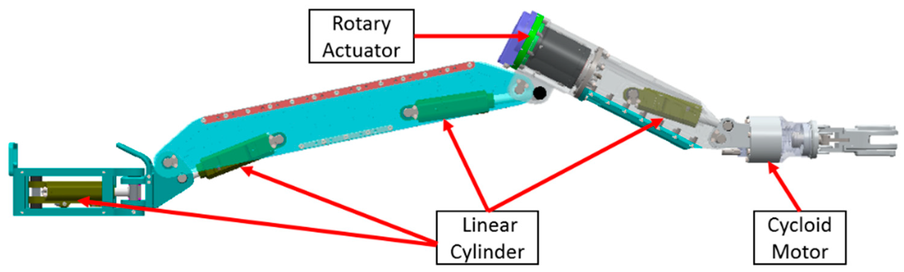
2.1. System Description

Hydraulic cylinders are used as the actuators of typical joints in deep-sea hydraulic manipulator systems. The motion and force of deep-sea hydraulic manipulators need to be provided by these joints. The schematic diagram of the system is shown in Figure 2.

$P_{1c}$ and $P_{2c}$ are the pressures in the forward and return chambers of the cylinder, respectively; $Q_{1c}$ and $Q_{2c}$ represent the supply and return flow rate to the forward and return chambers, respectively; $A_1$ and $A_2$ are the areas facing the forward and return chambers, respectively; $x_p$ is the displacement of the piston; $m$ is the equivalent mass of the load; $b$ is the equivalent damping coefficient; and $F_l\left(t\right)$ is the total external load force. $P_{1s}$ and $P_{1s}$ are the pressures at port A and port B of the servo valve, respectively; $Q_{1s}$ and $Q_{2s}$ represent the flow out of and into the servo valve, respectively; and $P_s$ and $P_0$ are the supply and return pressures, respectively.

2.2. Pipeline Model

G et al. defined four causal representations of a single pipeline [35]. The pipelines are connected to a servo valve at one port and a chamber at the other port in deep-sea hydraulic manipulator systems. The transfer functions for the two applied configurations are

$$\left[\begin{array}{c}{P}_d\left(s\right)\\ Q_u\left(s\right)\end{array}\right]=\left[\begin{array}{cc}\frac{1}{\cosh \mathsf{\Gamma }(s)}& -\frac{Z_c(s)\sinh \mathsf{\Gamma }(s)}{\cosh \mathsf{\Gamma }(s)}\\ \frac{\sinh \mathsf{\Gamma }(s)}{Z_c(s)\cosh \mathsf{\Gamma }(s)}& \frac{1}{\cosh \mathsf{\Gamma }(s)}\end{array}\right]\left[\begin{array}{c}{P}_u\left(s\right)\\ Q_d\left(s\right)\end{array}\right]$$

(1)

$$\left[\begin{array}{c}{P}_u\left(s\right)\\ Q_d\left(s\right)\end{array}\right]=\left[\begin{array}{cc}\frac{1}{\cosh \mathsf{\Gamma }(s)}& \frac{Z_c(s)\sinh \mathsf{\Gamma }(s)}{\cosh \mathsf{\Gamma }(s)}\\ -\frac{\sinh \mathsf{\Gamma }(s)}{Z_c(s)\cosh \mathsf{\Gamma }(s)}& \frac{1}{\cosh \mathsf{\Gamma }(s)}\end{array}\right]\left[\begin{array}{c}{P}_d\left(s\right)\\ Q_u\left(s\right)\end{array}\right]$$

(2)

where $\mathsf{\Gamma }(s)$ and $Z_c(s)$ represent the propagation operator and line characteristic impedance, respectively.

Since the valve-controlled cylinder studied in this work is a highly nonlinear system, the analysis should be performed in the time domain. The description of the pipeline dynamics in the frequency domain is not suitable. To deal with this problem, modal approximation models are adopted in this paper.

The transfer functions Equations (1) and (2) are dual to each other; thus, only Equation (1) is chosen to be discussed. The core of modal approximation is to use a finite number of modes to approximate the infinite sum of the modal contributions for the outputs [32].

The output can be expressed by the sum of the modal contributions as

$$\left[\begin{array}{l}{P}_d\\ Q_u\end{array}\right]=\left[\begin{array}{l}{\displaystyle \sum _{i=1}^n{P}_{di}}\\ {\displaystyle \sum _{i=1}^n{Q}_{di}}\end{array}\right]$$

(3)

For the ith mode, the state space equation can be given as [32]

$$\left[\begin{array}{l}{\dot{P}}_{di}\\ {\dot{Q}}_{ui}\end{array}\right]=\left[\begin{array}{cc}0& \left(-1\right){}^{i+1}{Z}_0{\omega }_{ci}\\ -\frac{\left(-1\right){}^{i+1}{\omega }_{ci}}{Z_0{\alpha }^2}& -\frac{32\nu \beta }{d^2\alpha }\end{array}\right]\left[\begin{array}{l}{P}_{di}\\ Q_{ui}\end{array}\right]+\left[\begin{array}{cc}0& \frac{8\nu Z_0}{d^2{D}_n}\\ -\frac{8\nu }{d^2{Z}_0{D}_n{\alpha }^2}& 0\end{array}\right]\left[\begin{array}{l}{P}_u\\ Q_d\end{array}\right]$$

(4)

where $\alpha ,\beta$ are frequency-dependent modification factors and can be obtained from [15]. ${\omega }_{ci}$ represents the modal undamped natural frequencies; $D_n$ is the dissipation number;$Z_o$ is the line impedance constant; and $c$ is the speed of sound in the oil, given by

$${\omega }_{ci}=\frac{4\nu }{d^2}\frac{\pi \left(i-\frac{1}{2}\right)}{D_n},i=1,2,3\dots n$$

(5)

$$D_n=\frac{4l\nu }{c{d}^2}$$

(6)

$$Z_o=\frac{4\rho c}{\pi d^2}$$

(7)

$$c=\sqrt{\frac{{\beta }_e}{\rho }}$$

(8)

where $v$ is the kinetic viscosity of oil; $\rho$ represents the fluid density; $d$ is the diameter of the pipeline; and $l$ is the length of the pipeline.

The finite number of modes in the model causes the steady state properties to be incorrect. Suppose that matrix $A_i$ is the feedback matrix and that $B_i$ is the input matrix. By introducing the input matrix modifier $G$ [15], each mode can be expressed:

$$\left[\begin{array}{c}{\dot{P}}_{di}\\ {\dot{Q}}_{ui}\end{array}\right]=A_i\left[\begin{array}{l}{P}_{di}\\ Q_{ui}\end{array}\right]+B_{i}G\left[\begin{array}{l}{P}_u\\ Q_d\end{array}\right]$$

(9)

where $A_i=\left[\begin{array}{cc}0& \left(-1\right){}^{i+1}{Z}_0{\omega }_{ci}\\ -\frac{\left(-1\right){}^{i+1}{\omega }_{ci}}{Z_0{\alpha }^2}& -\frac{32\nu \beta }{d^2\alpha }\end{array}\right]$, $B_i=\left[\begin{array}{cc}0& -\frac{8\nu Z_0}{d^2{D}_n}\\ -\frac{8\nu }{d^2{Z}_0{D}_n{\alpha }^2}& 0\end{array}\right]$, and $G=-{\left({\displaystyle \sum _{i=1}^n{A}_i^{-1}{B}_i}\right)}^{-1}\left[\begin{array}{ll}1& -8Z_0{D}_n\\ 0& 1\end{array}\right]$.

Thus, for the n-mode approximation, the steady-state value is

$${\left[\begin{array}{l}{P}_d\\ Q_u\end{array}\right]}_{ss}={{\displaystyle \sum _{i=1}^n\left[\begin{array}{l}{P}_{di}\\ Q_{ui}\end{array}\right]}}_{ss}=-{\displaystyle \sum _{i=1}^n\left(A_i^{-1}{B}_i\right)}G{\left[\begin{array}{l}{P}_u\\ Q_d\end{array}\right]}_{ss}$$

(10)

2.3. Valve-Controlled Cylinder Servo System Dynamics

The dynamics of the hydraulic cylinder can be described by

$$P_{1c}{A}_1-P_{2c}{A}_2=m{\ddot{x}}_p+b{\dot{x}}_p+k{x}_p+F_l$$

(11)

The pressure dynamics of the forward and return chambers can be written as

$$\{\begin{array}{l}\frac{V_1}{{\beta }_e}{\dot{P}}_{1c}=Q_{1c}-A_1{\dot{x}}_p-c_i\left(P_{1c}-P_{2c}\right)-c_e{P}_{1c}\\ \frac{V_2}{{\beta }_e}{\dot{P}}_{2c}=-Q_{2c}+A_2{\dot{x}}_p+c_i\left(P{c}_1-P_{2c}\right)-c_e{P}_{2c}\end{array}$$

(12)

where $V_1=V_{10}+A_1{x}_p$ represents the control volumes of the forward chamber; $V_2=V_{20}-A_2{x}_p$ represents the control volumes of the return chamber; $V_{10}$ and $V_{20}$ are the initial control volumes of the two chambers, respectively; ${\beta }_e$ is the effective bulk modulus of oil; and $c_i$ and $c_e$ are the internal and external leakage coefficients, respectively. $Q_{1s}$ and $Q_{2s}$ can be modeled by

$$\{\begin{array}{l}{Q}_{1s}=k_q{x}_v\left[s\left(x_v\right)\sqrt{P_s-P_{1s}}+s\left(-x_v\right)\sqrt{P_{1s}-P_0}\right]\\ Q_{2s}=k_q{x}_v\left[s\left(x_v\right)\sqrt{P_{2s}-P_0}+s\left(-x_v\right)\sqrt{P_s-P_{2s}}\right]\end{array}$$

(13)

Define

$$s(\ast )=\{\begin{array}{l}1,if\ast \ge 0\\ 0,if\ast <0\end{array}$$

(14)

where $k_q$ is the flow gain of the servo valve, and $x_v$ is the displacement of the servo valve.

The displacement of the servo valve spool can be related to the input current by the first-order system [36]

$${\dot{x}}_v=-\frac{1}{{\tau }_v}{x}_v+\frac{k_i}{{\tau }_v}u$$

(15)

where ${\tau }_v$ is the time constant, and $k_i$ is the current gain.

2.4. State Space Model of the System and Its Simplification

The influence of long pipelines between the servo valve and the cylinder chambers on the hydraulic system is mainly reflected in pressure, and the impact on flow rate is ignored, i.e.,$Q_{1c}=Q_{1s}$ and $Q_{2c}=Q_{2s}$. Define the state variables $x={\left[x_1,x_2,x_3,x_4,x_5\right]}^T={\left[x_p,{\dot{x}}_p,P_{1c},P_{2c},x_v\right]}^T$, and considering Equations (1)–(6), the dynamics of the HDU can be expressed in the state space form as

$$\{\begin{array}{l}{\dot{x}}_1=x_2\\ {\dot{x}}_2=-\frac{k}{m}{x}_1-\frac{b}{m}{x}_2+\frac{A_1}{m}{x}_3-\frac{A_2}{m}{x}_4-\frac{F_f}{m}\\ {\dot{x}}_3=\frac{{\beta }_e}{V_{10}+A_1{x}_1}\left(k_q{x}_5\left[s\left(x_5\right)\sqrt{P_s-P_{1s}}+s\left(-x_5\right)\sqrt{P_{1s}-P_0}\right]-A_1{x}_2\right)\\ {\dot{x}}_4=\frac{{\beta }_e}{V_{20}-A_2{x}_1}\left(-k_q{x}_5\left[s\left(x_5\right)\sqrt{P_{2s}-P_0}+s\left(-x_5\right)\sqrt{P_s-P_{2s}}\right]+A_2{x}_2\right)\\ {\dot{x}}_5=-\frac{1}{{\tau }_v}{x}_5+\frac{k_a}{{\tau }_v}u\end{array}$$

(16)

Define ${\overline{x}}_3=x_3-n{x}_4$,${\overline{x}}_4=x_5$ and $n=A_2/A_1$. We can rewrite Equation (17) in strictly a feedback form as

$$\{\begin{array}{l}{\dot{x}}_1=x_2\\ {\dot{x}}_2=-\frac{k}{m}{x}_1-b\frac{1}{m}{x}_2+\frac{A_1}{m}{\overline{x}}_3+d_2\\ {\dot{\overline{x}}}_3={\beta }_e\frac{1}{V_1}\left(k_q{\overline{x}}_4\left[s\left({\overline{x}}_4\right)\sqrt{P_s-P_{1s}}+s\left(-{\overline{x}}_4\right)\sqrt{P_{1s}-P_0}\right]-A_1{x}_2\right)\\ -n{\beta }_e\frac{1}{V_2}\left(-k_q{\overline{x}}_4\left[s\left({\overline{x}}_4\right)\sqrt{P_{2s}-P_0}+s\left(-{\overline{x}}_4\right)\sqrt{P_s-P_{2s}}\right]+A_2{x}_2\right)\\ {\dot{\overline{x}}}_4=-\frac{1}{{\tau }_v}{\overline{x}}_4+\frac{k_a}{{\tau }_v}u\end{array}$$

(17)

Then, define parameters ${\theta }_1=\frac{k}{m}$, ${\theta }_2=\frac{b}{m}$, ${\theta }_3=\frac{A_1}{m}$, ${\theta }_4={\beta }_e$, ${\theta }_5={\beta }_e{k}_q$, ${\theta }_6=\frac{1}{{\tau }_v}$, ${\theta }_7=\frac{k_a}{{\tau }_v}$ and $d_2=\frac{F_l}{m}$ and substitute them into Equation (18). The state space Equation (18) is converted into

$$\{\begin{array}{l}{\dot{x}}_1=x_2\\ {\dot{x}}_2=-{\theta }_1{x}_1-{\theta }_2{x}_2+{\theta }_3{\overline{x}}_3+d_2\\ {\dot{\overline{x}}}_3=-{\theta }_4{f}_1{x}_2+{\theta }_5{f}_2{\overline{x}}_4\\ {\dot{\overline{x}}}_4=-{\theta }_6{\overline{x}}_4+{\theta }_{7}u\end{array}$$

(18)

where $\begin{array}{l}{R}_1=\left[s\left(x_4\right)\sqrt{P_s-P_{1s}}+s\left(-x_4\right)\sqrt{P_{1s}-P_0}\right]\\ R_2=\left[s\left(x_4\right)\sqrt{P_{2s}-P_0}+s\left(-x_4\right)\sqrt{P_s-P_{2s}}\right]\end{array}$, and $f_1=\frac{A_1}{V_1}+n\frac{A_2}{V_2},f_2=\frac{R_1}{V_1}+n\frac{R_2}{V_2}$.

The effective bulk modulus of oil ${\beta }_e$ is variable throughout the whole work process due to different temperatures and environmental pressures. The external load force $F_l$ is also uncertain. Thus, there exists uncertainty in parameters ${\theta }_4,{\theta }_5$.

Even though ${\beta }_e$ and $F_l$ are uncertain, they are all bounded and positive in practical systems.

$${\theta }_i\in {\mathsf{\Omega }}_{{\theta }_i}\triangleq \left[{\theta }_{\min },{\theta }_{\max }\right]i=4,5$$

(19)

$$\left|d_2\right|\le D$$

(20)

where ${\theta }_{\min }=\left[{\theta }_{4\min },{\theta }_{5\min }\right]$, ${\theta }_{\max }=\left[{\theta }_{4\max },{\theta }_{5\max }\right]$ and $D$ are known.

Let $\widehat{\theta }$ denote the estimate of $\theta$, and let the estimation error $\tilde{\theta }=\widehat{\theta }-\theta$. The adaptive law is designed later to derive estimates and to guarantee its boundary.

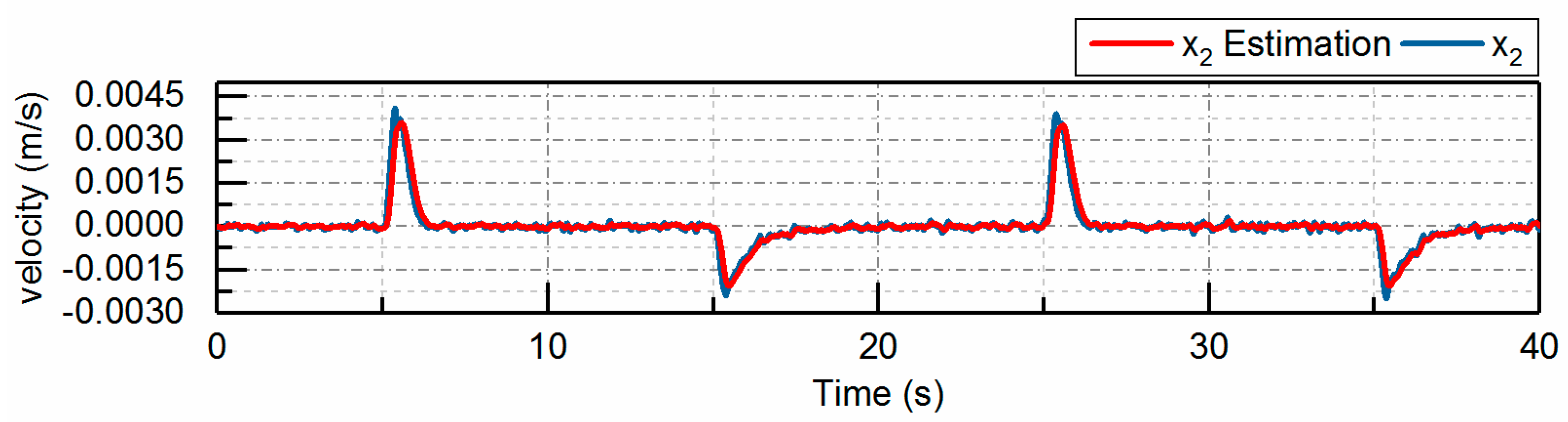
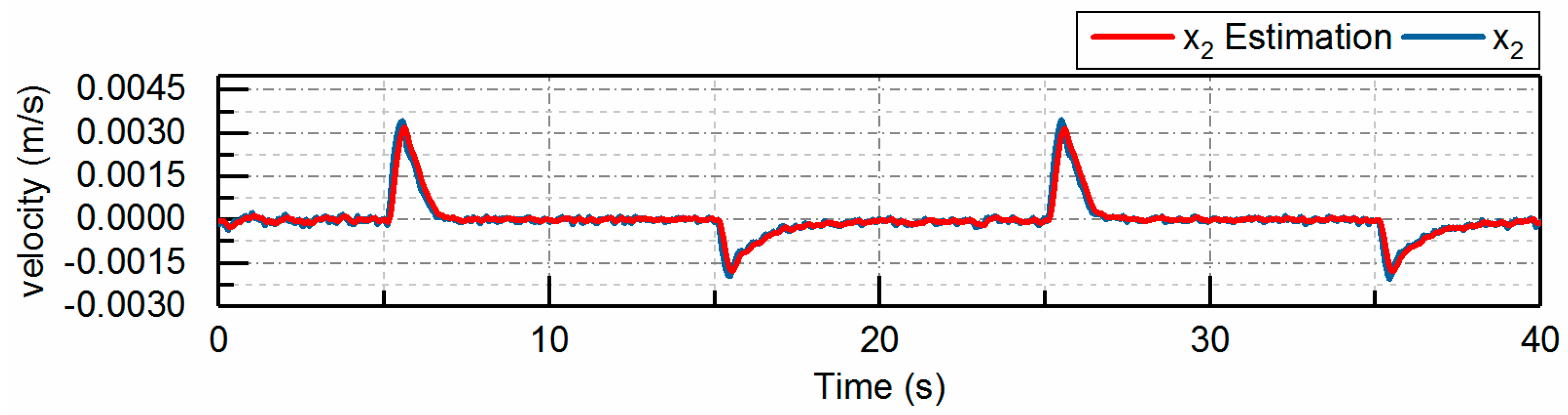
3. Extended State Observer Design

There is only a displacement sensor in the hydraulic cylinder, and only the displacement information $x_1$ is measurable. The velocity information obtained by differentiating the displacement cannot be used in the design of the controller directly; thus, an effective way to obtain the velocity information should be given. Moreover, the external disturbances $d_2$, which contain unknown disturbances and unmodeled items, cannot be known accurately. Thus, an extended state observer (ESO) was constructed to estimate the velocity of the piston and external disturbances.

It can be seen from the structural diagram in this paper that the displacement information $x_p$ and the pressure information $P_{1s}$ and $P_{2s}$ in the servo valve port can be measured by the sensors. The pressure information $P_{1c}$ and $P_{2c}$ at the port of the hydraulic cylinder can be obtained indirectly through the pipeline model, and $x_1,P_{1c},P_{2c}$ are used to build an estimation system.

The first two equations of Equation (19) can be rewritten as

$$\{\begin{array}{l}{\dot{x}}_1=x_2\\ {\dot{x}}_2=-{\widehat{\theta }}_1{x}_1-{\widehat{\theta }}_2{x}_2+{\widehat{\theta }}_3{x}_3+d_2\\ {\dot{d}}_2=h_2\left(t\right)\end{array}$$

(21)

${\widehat{x}}_1,{\widehat{x}}_2$ and ${\widehat{d}}_2$ are estimates of $x_1,x_2$ and $d_2$, respectively. An ESO can be constructed as [35]

$$\{\begin{array}{l}{\dot{\widehat{x}}}_1={\widehat{x}}_2+3{\omega }_0\left({\widehat{x}}_1-x_1\right)\\ {\dot{\widehat{x}}}_2=-{\widehat{\theta }}_1{\widehat{x}}_1-{\widehat{\theta }}_2{\widehat{x}}_2+{\widehat{\theta }}_3{x}_3+{\widehat{d}}_2+\\ {\dot{\widehat{d}}}_2={\omega }_0^3\left({\widehat{x}}_1-x_1\right)\end{array}3{\omega }_0^2\left({\widehat{x}}_1-x_1\right)$$

(22)

Define the estimation errors as ${\tilde{x}}_1={\widehat{x}}_1-x_1$. The dynamic state estimation error can be given as

$$\{\begin{array}{l}{\dot{\tilde{x}}}_1={\tilde{x}}_2-3{\omega }_0\left({\widehat{x}}_1-x_1\right)\\ {\dot{\tilde{x}}}_2={\tilde{d}}_2-3{\omega }_0^2\left({\widehat{x}}_1-x_1\right)\\ {\dot{\widehat{d}}}_2=h_2\left(t\right)-{\omega }_0^3\left({\widehat{x}}_1-x_1\right)\end{array}$$

(23)

The scaled estimation error can be defined as $\epsilon ={\left[{\epsilon }_1,{\epsilon }_2,{\epsilon }_3\right]}^T={\left[{\tilde{x}}_1,\frac{{\tilde{x}}_2}{{\omega }_0},\frac{{\tilde{d}}_2}{{\omega }_0^2}\right]}^T$.

Then, Equation (24) can be rewritten as

$$\dot{\epsilon }={\omega }_{0}A\epsilon +B\frac{h_2(t)}{{\omega }_0^2}$$

(24)

where $A=\left[\begin{array}{l}-310\\ -301\\ -100\end{array}\right]$, and $B={\left[0,0,1\right]}^T$, where A is a Hurwitz matrix. There exists a symmetric positive definite matrix P satisfying the following equation:

$$A^{T}P+PA=-I$$

(25)

4. Extended-State-Observer-Based Fuzzy Adaptive Backstepping Controller Design

4.1. Controller Design

In this section, the latter three sub-equations in (18) are chosen to design the backstepping controller. Let the load pressure $P_L=\left(A_1{P}_{1c}-A_2{P}_{2c}\right)/A_1={\overline{x}}_3$, and the output force of the hydraulic cylinder is indirectly controlled by controlling the load pressure. The dynamic surface control (DSC) technique is employed to avoid the “explosion of complexity” problem in the conventional backstepping controller.

Step 1: Define the errors of ${\overline{x}}_3$ and the desired load pressure ${\overline{x}}_{3d}$ as

$$e_3={\overline{x}}_3-{\overline{x}}_{3d}=P_L-P_{Ld}$$

(26)

The time derivative of Equation (27) becomes

$$\begin{array}{ll}{\dot{e}}_3& ={\dot{\overline{x}}}_3-{\dot{\overline{x}}}_{3d}\\ & =-{\theta }_4{f}_1{x}_2+{\theta }_5{f}_2{\overline{x}}_4-{\dot{\overline{x}}}_{3d}\\ & =-{\widehat{\theta }}_4{f}_1{x}_2+{\tilde{\theta }}_4{f}_1{x}_2+{\widehat{\theta }}_5{f}_2{\overline{x}}_4-{\tilde{\theta }}_5{f}_2{\overline{x}}_4-{\dot{\overline{x}}}_{3d}\end{array}$$

(27)

The first virtual control variable ${\overline{x}}_{4d}$ can be chosen as

$${\overline{x}}_{4d}=\frac{1}{{\widehat{\theta }}_5{f}_2}\left(-k_1{e}_3+{\widehat{\theta }}_4{f}_1{x}_2+{\dot{\overline{x}}}_{3d}\right)$$

(28)

where $k_1>0$ is the first controller gain; its value is generally large to enable the system to obtain a rapid response. ${\widehat{\theta }}_4,{\widehat{\theta }}_5$ represent the estimate of ${\theta }_4,{\theta }_5$, and the adaptive law is given by

$$\{\begin{array}{l}{\dot{\tilde{\theta }}}_4=-\frac{e_3{f}_1{x}_2}{{\lambda }_1}\\ {\dot{\tilde{\theta }}}_5=-\frac{e_3{f}_2{\overline{x}}_{4d}}{{\lambda }_2}\end{array}$$

(29)

where ${\lambda }_1,{\lambda }_2$ are positive constants.

A new virtual control variable ${\overline{x}}_{4f}$ can be obtained if ${\overline{x}}_{4d}$ is allowed to pass through a first-order filter as follows:

$$\tau {\dot{\overline{x}}}_{4f}+{\overline{x}}_{4f}={\overline{x}}_{4d},{\overline{x}}_{4f}\left(0\right)={\overline{x}}_{4d}\left(0\right)$$

(30)

where $\tau$ is the time constant of the filter, and its value is generally small; therefore, the filter has high accuracy.

Step 2: Define the errors of ${\overline{x}}_4$ and the desired displacement of the spool ${\overline{x}}_{4d}$ as

$$e_4={\overline{x}}_4-{\overline{x}}_{4f}$$

(31)

The time derivative of Equation (32) becomes

$${\dot{e}}_4={\dot{\overline{x}}}_4-{\dot{\overline{x}}}_{4f}=-{\theta }_6{\overline{x}}_4+{\theta }_{7}u-{\dot{\overline{x}}}_{4f}$$

(32)

The control input $u$ can be designed as

$$u=\frac{1}{{\theta }_7}\left[{\theta }_6{\overline{x}}_4-{\widehat{\theta }}_5{f}_2{e}_3+{\dot{x}}_{4f}-k_2{e}_4\right]$$

(33)

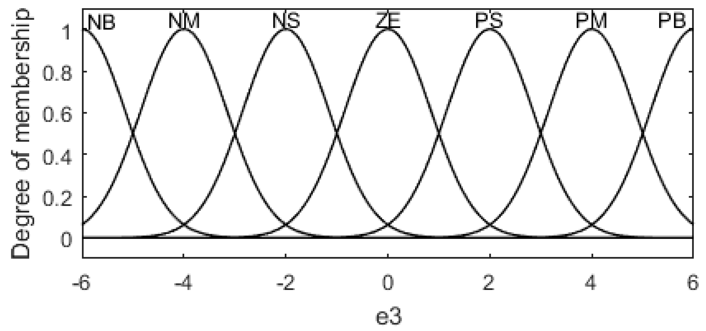
4.2. Fuzzy Self-Tuners

The working environment pressure of the deep-sea hydraulic manipulator ranges from 0 to 115 MPa, and the large-scale change in environmental pressure leads to a significant change in some parameters of the system. The large change in oil viscosity is taken into account in this study. The fixed control parameters make it difficult to obtain the expected deviation dynamic characteristics and even lead to system instability. In order to ensure that the system can maintain good performance in a large range of environmental pressure, fuzzy logic is employed to design self-tuners that can automatically adjust the control parameters.

The two inputs of the fuzzy structure are the load pressure $e_3$ and its derivative ${\dot{e}}_3$. The input domains of $e_3$ and ${\dot{e}}_3$ are both $\left\{-6,6\right\}$, which are obtained from the absolute values of $e_3$ and ${\dot{e}}_3$ through the scale factors. The outputs of the fuzzy structure are $u_1,u_2$. The domain is ascertained as $\left\{-3,3\right\}$ of $u_1$ and $\left\{-1,1\right\}$ of $u_2$.

Seven linguistic terms are used for both the input and output variables: negative big (NB), negative middle (NM), negative small (NS), zero (ZO), positive small (PS), positive middle (PM) and positive big (PB). The membership functions are shown in Figure 3 and Figure 4.

These gaussian shape MFs can be expressed as

$$\mu \left(x_i\right)=e^{-\frac{{\left(x_i-c_{ji}\right)}^2}{2{\sigma }_{ji}{}^2}},j=1,2,\dots ,N$$

(34)

where $c_{ji}$ is the mid-value of the $j$ th Gauss bell, and the value of ${\sigma }_{ji}>0$; $N$ is the number of Gauss bells.

The fuzzy rules obtained from engineering experience and technical attempts are described in

Table 1. Fuzzy rules.

${\mathbf{u}}_1,{\mathbf{u}}_2$		${\mathbf{e}}_3$
		NB	NM	NS	ZO	PS	PM	PB
${\dot{e}}_3$	NB	PB/NB	PB/NB	PM/NM	PM/NM	PS/NS	ZO/NS	ZO/ZO
	NM	PB/NB	PB/NB	PM/NM	PM/NM	PS/NS	ZO/ZO	ZO/ZO
	MS	PM/NM	PM/NM	PM/NS	PS/NS	ZO/ZO	NS/PS	NM/PS
	ZO	PM/NM	PS/NS	PS/NS	ZO/ZO	NS/PS	NM/PS	NM/PM
	PS	PS/NS	PS/NS	ZO/ZO	NS/PS	NS/PS	NM/PM	NM/PM
	PM	ZO/ZO	ZO/ZO	NS/PS	NM/PM	NM/PM	NM/PB	NB/PB
	PB	ZO/ZO	NS/ZO	NS/PS	NM/PM	NM/PM	NB/PB	NB/PB

.

The MAX–MIN aggregation method is used here, and the output can be computed as

$$\Delta k_i=\frac{{\displaystyle \sum _{j=i}^M{\mu }_j{w}_j}}{{\displaystyle \sum _{j=i}^M{\mu }_j}}$$

(35)

where ${\mu }_j$ and ${\omega }_j$ are the height and the weight of the output obtained from the jth rule, respectively.

Through fuzzy logic knowledge, the fuzzy self-tuners that tune control parameters ($k_1,k_2$) can be established by using the following equation:

$$k_{if}=k_{io}+u_i\Delta k_i,i=1,2$$

(36)

where $u_i$ is the parameter obtained from the output of the fuzzy self-tuner; and $\Delta k_i=k_{if\max }-k_{if\min }$ and $k_{if\max },k_{if\min }$ are the maximum and minimum values of $k_{if}$ determined from Equation (37) and the experiments, respectively.

4.3. Stability Analysis

The filtering error of the low-pass filter Equation (31) is defined as

$$s={\overline{x}}_{4f}-{\overline{x}}_{4d}$$

(37)

Then, ${\overline{x}}_4$ can be expressed as

$${\overline{x}}_4={\overline{x}}_{4f}+e_4+s$$

(38)

The time derivative of Equation (27) can be rewritten as

$$\begin{array}{ll}{\dot{e}}_3& ={\dot{x}}_3-{\dot{x}}_{3d}\\ & =-{\theta }_4{f}_1{x}_2+{\theta }_5{f}_2{\overline{x}}_4-{\dot{x}}_{3d}\\ & =-{\widehat{\theta }}_4{f}_1{x}_2+-{\tilde{\theta }}_4{f}_1{x}_2+{\widehat{\theta }}_5{f}_2\left(\frac{1}{{\widehat{\theta }}_5{f}_2}\left(-k_1{e}_3+{\widehat{\theta }}_4{f}_1{x}_2+{\dot{x}}_{3d}\right)+e_4+s\right)\\ & -{\tilde{\theta }}_5{f}_2\left({\overline{x}}_{4f}+e_4+s\right){\dot{x}}_{3d}\\ & =-k_{1f}{e}_3+{\theta }_5{f}_2\left(e_4+s\right)+{\tilde{\theta }}_4{f}_1{x}_2-{\tilde{\theta }}_5{f}_2{\overline{x}}_{4f}\end{array}$$

(39)

The time derivative of Equation (32) can be rewritten as

$$\begin{array}{ll}{\dot{e}}_4& ={\dot{\overline{x}}}_4-{\dot{\overline{x}}}_{4f}\\ & =-{\theta }_6{\overline{x}}_4+{\theta }_7\left(\frac{1}{{\theta }_7}\left[{\theta }_6{\overline{x}}_4-{\widehat{\theta }}_5{f}_2{e}_3\left(e_4+s\right)+{\dot{\overline{x}}}_{4f}-k_{2f}{e}_4\right]\right)\\ & =-{\widehat{\theta }}_5{f}_2{e}_3-k_{2f}{e}_4\end{array}$$

(40)

By substituting Equation (35) into Equation (31), the new virtual control variable derivative is obtained as

$${\dot{\overline{x}}}_{4f}=-\frac{s}{\tau }$$

(41)

The time derivative of Equation (35) can be obtained as

$$\dot{s}={\dot{x}}_{4d}-{\dot{\overline{x}}}_{4f}=-\frac{s}{\tau }-{\dot{\overline{x}}}_{4f}$$

(42)

Based on Equation (37), Equation (38) and Equation (43), there is a nonnegative continuous function B, such that

$$\dot{s}\le -\frac{s}{\tau }+B\left(e_3,s,x_{3d},{\dot{x}}_{3d},{\ddot{x}}_{3d}\right)$$

(43)

Consider the following compact sets:

$$\begin{array}{l}{\mathsf{\Omega }}_1=\left\{\left(x_{3d},{\dot{x}}_{3d},{\ddot{x}}_{3d}\right):x_{3d}^2+{\dot{x}}_{3d}^2+{\ddot{x}}_{3d}^2\le g\right\}\\ {\mathsf{\Omega }}_2=\left\{e_3^2+e_4^2+s^2\le 2N\right\}\end{array}$$

(44)

Note that the set ${\mathsf{\Omega }}_1\times {\mathsf{\Omega }}_2$ is also compact, and there exists a positive constant $M$, such that $B\le M$ on ${\mathsf{\Omega }}_1\times {\mathsf{\Omega }}_2$.

Define a Lyapunov function candidate as

$$V=\frac{1}{2}{e}_3^2+\frac{1}{2}{\lambda }_1{\tilde{\theta }}_4^2+\frac{1}{2}{\lambda }_2{\tilde{\theta }}_5^2+\frac{1}{2}{e}_4^2+\frac{1}{2}{s}^2$$

(45)

By differentiating $V$, obtain

$$\begin{array}{ll}\dot{V}& =e_3{\dot{e}}_3+{\lambda }_1{\tilde{\theta }}_4{\dot{\tilde{\theta }}}_4+{\lambda }_2{\tilde{\theta }}_5{\dot{\tilde{\theta }}}_5+e_4{\dot{e}}_4+s\dot{s}\\ & =e_3\left(-k_{1f}{e}_3+{\theta }_5{f}_2\left(e_4+s\right)+{\tilde{\theta }}_4{f}_1{x}_2-{\tilde{\theta }}_5{f}_2{\overline{x}}_{4d}\right)+{\lambda }_1{\tilde{\theta }}_4\left(-\frac{e_3{f}_1{x}_2}{{\lambda }_1}\right)\\ & +{\lambda }_2\tilde{\theta }\left(-\frac{e_3{f}_2{\overline{x}}_{4d}}{{\lambda }_2}\right)+e_4\left(-{\widehat{\theta }}_5{f}_2{e}_3-k_{2f}{e}_4\right)+s\left(-\frac{s}{\tau }-{\dot{\overline{x}}}_{4f}\right)\\ & =-k_{1f}{e}_3^2-k_{2f}{e}_4^2+{\theta }_5{f}_2{e}_{3}s+s\left(-\frac{s}{\tau }-{\dot{\overline{x}}}_{4f}\right)\end{array}$$

(46)

Using Young’s inequalities $2xy\le x^2+y^2$, the time derivative can be written as

$$\begin{array}{ll}\dot{V}& =-k_{1f}{e}_3^2-k_{2f}{e}_4^2+{\theta }_5{f}_2{e}_{3}s+s\dot{s}\\ & \le -k_{1f}{e}_3^2-k_{2f}{e}_4^2+{\theta }_5{f}_2{e}_{3}s+\left(-\frac{s^2}{\tau }+\left|B\right|\left|s\right|\right)\\ & \le -k_{1f}{e}_3^2-k_{2f}{e}_4^2+\frac{{\theta }_5{f}_2}{2}{e}_3^2+\frac{{\theta }_5{f}_2}{2}{s}^2+\left(-\frac{s^2}{\tau }+\left|B\right|\left|s\right|\right)\\ & \le \left(\frac{{\theta }_5{f}_2}{2}-k_{1f}\right)e_3^2-k_{2f}{e}_4^2+\left(\frac{{\theta }_5{f}_2}{2}-\frac{1}{\tau }+\frac{B^2}{2}\right)s^2\end{array}$$

(47)

Select appropriate parameters that meet the following conditions:

$$k_{1f}\ge \frac{{\theta }_5{f}_2}{2}+r,k_{2f}\ge r,\frac{1}{\tau }\ge \frac{1}{2}+\frac{M^2}{2}+r$$

where $r$ is a small positive constant, then

$$\dot{V}\le -r\left(e_3^2+e_4^2+s^2\right)+\left(\frac{B^2}{2M}-\frac{1}{2}\right)s^2{M}^2=-2rV+\left(\frac{B^2}{2M}-\frac{1}{2}\right)s^2{M}^2$$

(48)

According to $B\le M$, derive

$$\dot{V}\le -2rV$$

(49)

Thus, all the signals are uniformly ultimately bounded.

Figure 5 shows the proposed extended-state-observer-based fuzzy adaptive backstepping controller. A pipeline model is established from which the pressures on the cylinder port can be obtained to design the extended state observer and controller. Moreover, an extended state observer is designed to obtain the unmeasurable state, including the velocity of the piston and external disturbances. Then, the designed adaptive law is used to adapt to the uncertainty of parameters. The backstepping controller is constructed to realize the force control of the system, and a fuzzy self-tuner is designed to adjust the backstepping control parameters to guarantee dynamic performance under the large-scale change in environmental pressure.

5. Experiment and Discussion

5.1. Experimental Setup

To verify the proposed control strategies, we established an experimental platform, as shown in Figure 6, and its schematic is shown in Figure 7. The hydraulic cylinder with a 55 mm bore and a 25 mm rod was connected to a three-position four-way servo valve via 3.747 m-long pipelines with 4 mm inside diameters. A force sensor was installed on the piston, and the force signal from the force sensor was used to verify the proposed force feedback method. Pressures were measured by analog pressure sensors installed in the valve pack at the exit port of the spool valve. The xPC rapid prototype technology was employed for the control system, which consisted of a host computer, a target computer, a data acquisition card and a servo amplifier board. An industrial computer installed with the xPC target real-time operating system was used as the target computer; the card PCI6229 containing A/D data acquisition and D/A signal driven was also installed on the target computer. A laptop computer installed with MATLAB/Simulink and Microsoft Visual Studio software served as the host computer. The servo amplifier board converted the voltage signal generated by the target computer into a current signal to drive the servo valve. The proposed and compared control algorithms were programmed by MATLAB/Simulink and were compiled to C code by Microsoft Visual Studio on the host computer, and then they were downloaded to the target computer for execution. A time of 0.01 s was selected as the sampling period to perform the control verification. The main physical parameters of the system are presented in

Table 2. Parameters of the system.

Parameters	Value	Parameters	Value
${\tau }_v$	1/1068	$k_q$	4.66 × 10−4
$k_i$	0.006	$\rho$	850 kg/m3
$d$	0.004 m	$P_s$	15 MPa
$l$	3.474 m	$P_0$	0 MPa
$A_1$	2.375 × 10−3 m2	$m$	17.8 kg
$A_2$	1.885 × 10−3 m2	$b$	25
$V_{10}$	7.55 × 10−5 m3	$k$	5 × 107 N/m
$V_{20}$	7.55 × 10−5 m3

.

The initial values of the uncertain parameters were set to be ${\theta }_4={\beta }_e=7\times {10}^8$ and ${\theta }_5=3.262\times {10}^5$. The bounds of the uncertain parameters were set to be ${\theta }_{4\min }=6\times {10}^8$, ${\theta }_{5\min }=2.796\times {10}^5$, ${\theta }_{4\max }=18\times {10}^8$ and ${\theta }_{5\max }=8.388\times {10}^5$.

5.2. Experimental Conditions and Methods

The ambient pressure increases with the increase in seawater depth, which in turn increases the viscosity of the oil. In this study, we simulated different working water depths with hydraulic oils of different viscosities. We selected 10# aviation hydraulic oil as the working medium of deep-sea hydraulic manipulator systems because its viscosity is less affected by pressure changes. Research on the viscosity–pressure characteristics of 10# aviation hydraulic oil was conducted [37].

To verify the applicability of the proposed method to the full-ocean-depth environment, three typical operating depths of 0 m, 4500 m and 11,000 m below the water surface with ambient pressures of 0 MPa, 45 MPa and 115 MPa were selected for the study. We found that the viscosity of 32# oil at normal pressure and 17 °C is 92.96 [38], which is the same as that of YH10 oil at 45 MPa and 2 °C, so 32# oil was used to simulate the 45 MPa ambient pressure, i.e., the depth of 4500 m. We found that the viscosity of 150# oil at normal pressure and 26 °C is 297.74 [35], which is the same as that of 10# oil at 115 MPa and 2 °C, so 150# oil was used to simulate the 115 MPa ambient pressure, i.e., the depth of 11,000 m. The underwater power unit was placed in a water tank, as shown in Figure 7, and ice cubes were added to the water tank to ensure that the underwater power unit worked at the required temperature.

5.3. Effectiveness of the Proposed Method

Before the proposed controller was applied in the real control system, the effectiveness of the pipeline model and the force control method based on pressure feedback were confirmed by experiments. Friction was ignored in this study; the output force of the hydraulic cylinder could be considered to be obtained by multiplying the load pressure by the effective area of the piston. The force results are plotted in Figure 8, Figure 9 and Figure 10.

The pressures at the port of the servo valve were used as feedback. The output force was measured by the force sensor installed at the end of the piston. Figure 8 shows that there was a considerable deviation between the force obtained by directly using the pressures measured at the servo valve port as the feedback and the force measured by the force sensor. The force calculated by pressures in the cylinder chambers, which were estimated by the pipeline model, was consistent with that measured by the force sensor. When the oil medium was changed to 32# and 150#, as shown in Figure 9 and Figure 10, the force obtained by the proposed method was still consistent with that measured by the force sensor.

5.4. Comparative Experimental Results

To demonstrate the effectiveness of the proposed controller, the following three controllers were compared.

1.

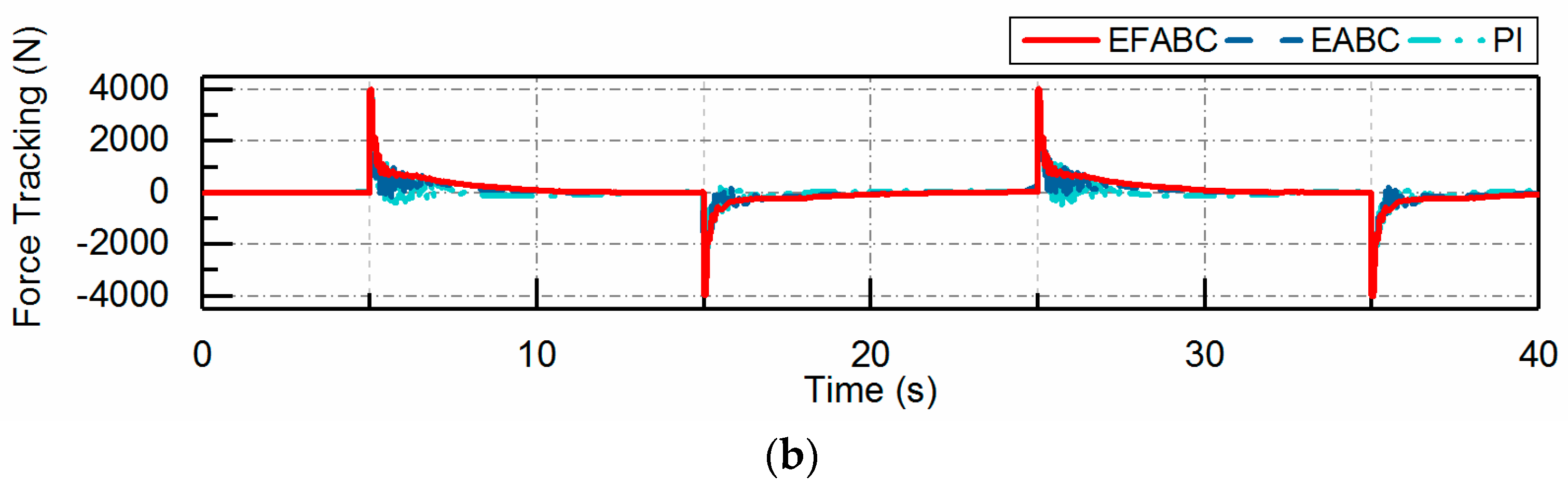
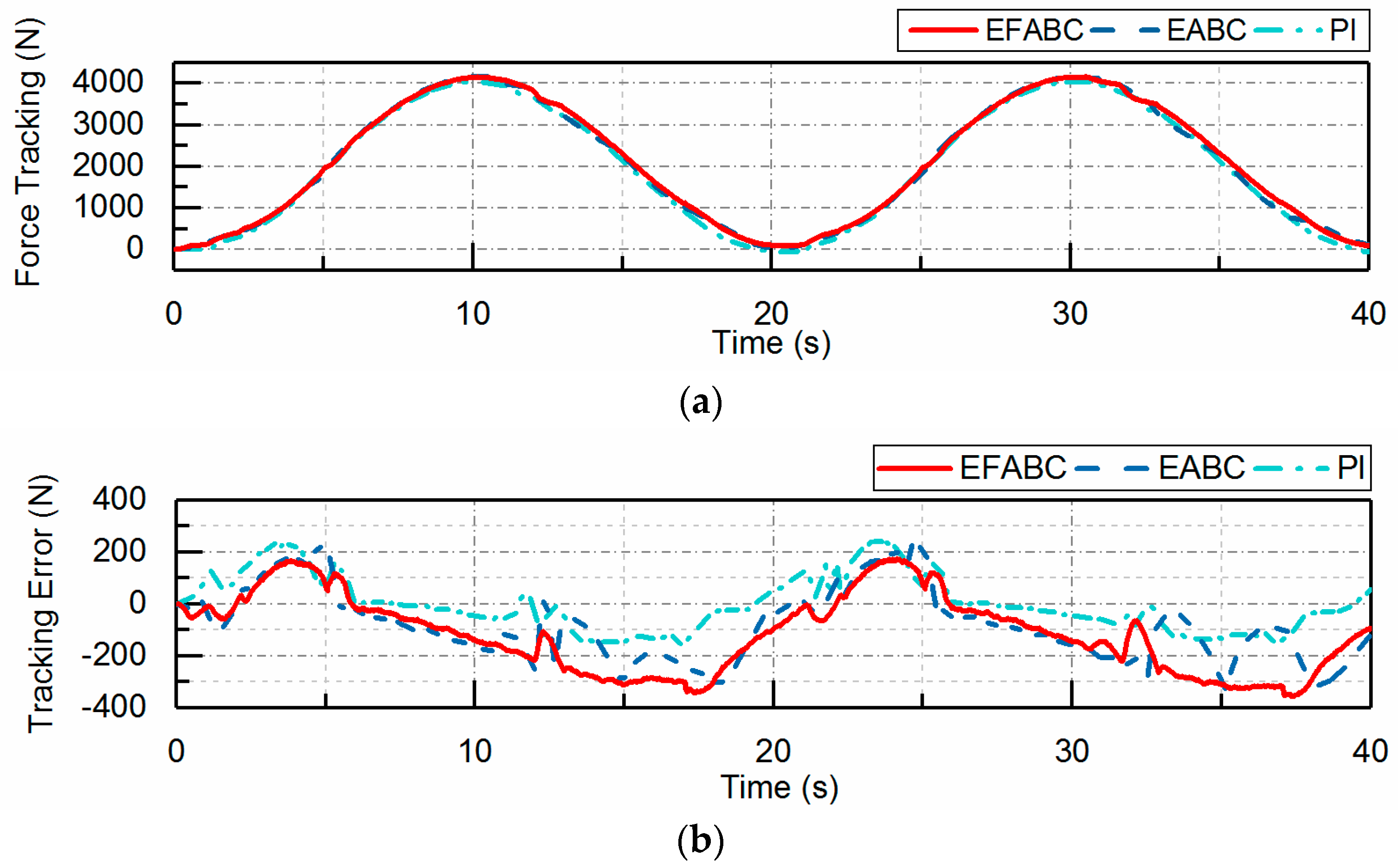
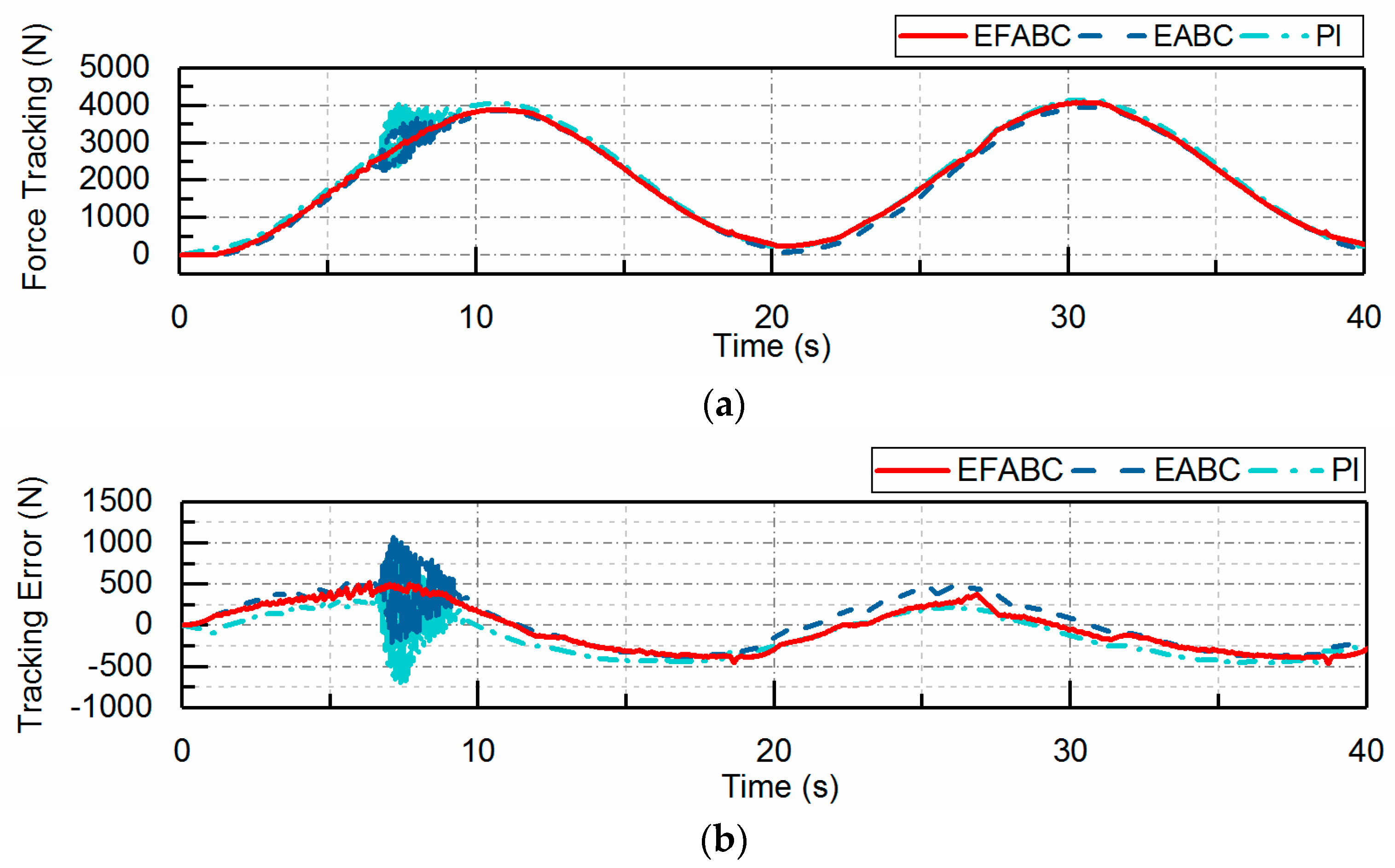
PI: The proportional–integral controller is commonly applied in industries. The control command is obtained from $u=k_{p}e+k_{i}ed(e)$, and the PI gains are $k_p=0.002,k_i=0.005$, which achieved good force tracking performance with YH10.

2.

EABC: The extended-state-observer-based adaptive backstepping controller, backstepping technology and adaptive updating law were employed based on an extended state observer to address parameter uncertainties and external disturbances. The control command was computed by (38), in which the gains were $k_1=5\times {10}^5,k_2=1.1\times {10}^5$ and ${\omega }_0=10$.

3.

EFABC: The extended-state-observer-based fuzzy adaptive backstepping controller with fuzzy logic was employed to design self-tuners, which could automatically adjust the control parameters based on EABC. The initial value of control gains was the same as EABC.

In order to compare the force tracking performance of the three different controllers, two different types of reference forces were selected: square wave and sine wave. The amplitudes were 4000 N, and the frequencies were 0.05 Hz.

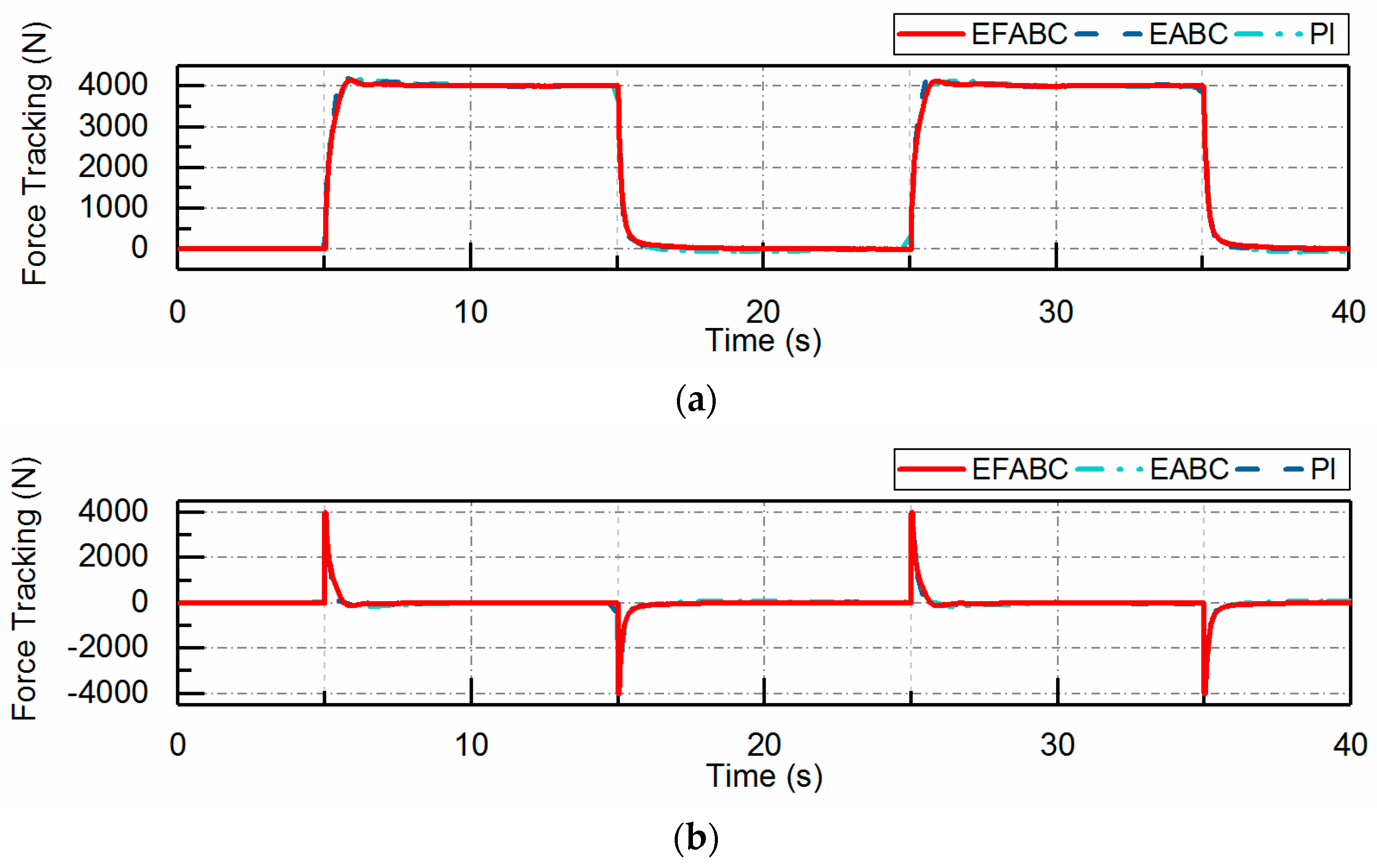
5.4.1. Case I: Square Wave

In the first case, a square wave reference force was utilized, which was not satisfactory. The experimental results are presented in Figure 11, Figure 12, Figure 13, Figure 14, Figure 15 and Figure 16. In addition, the steady state value error $e_S$, the maximum deviation $\delta$ and the adjust time $t_s$ of the first rising phase were selected as indexes to assess the performance of the three controllers and are summarized in

Table 3. Performance indexes with square reference force.

Index	10 # (0 m)			32 # (4500 m)			150 # (11,000 m)
	${\mathbf{t}}_{\mathbf{s}10}$	${\mathbf{e}}_{\mathbf{s}10}$	${\mathsf{\delta }}_{10}$	${\mathbf{t}}_{\mathbf{s}32}$	${\mathbf{e}}_{\mathbf{s}32}$	${\mathsf{\delta }}_{32}$	${\mathbf{t}}_{\mathbf{s}150}$	${\mathbf{e}}_{\mathbf{s}150}$	${\mathsf{\delta }}_{150}$
PI	4.24	3.81%	8.65	>10	-	-	>10	-	-
EABC	3.50	4.72%	4.99	>10	-	-	5.29	6.25%	−1.78
EFABC	2.24	3.16%	6.19	1.31	1.13	5.89	5.88	0.60%	−4.22

. As seen from Figure 11, Figure 13 and Figure 15, the proposed controller took the shortest time of 2.24 s to reach a steady state when using 10# as the medium. When 32# was used, it took the shortest time of 1.31 s, and the other two controllers could not reach a steady state within 10 s. With 150# as the medium, it took 5.88 s, longer than EABC, which had obvious overshoot oscillations. The maximum deviation of EFABC was the smallest. Thus, the proposed EFABC controller had the best force control performance among the compared three controllers when using oil with different viscosities as the working medium. The tracking error of EFABC converged to zero in 10 s. The estimation of velocity when working under different viscosities of oil are shown in Figure 12, Figure 14 and Figure 16. As shown, the estimated velocity derived from the ESO could track the velocity obtained by the displacement differentiation well and had low noise, which contributed to improving the force control performance.

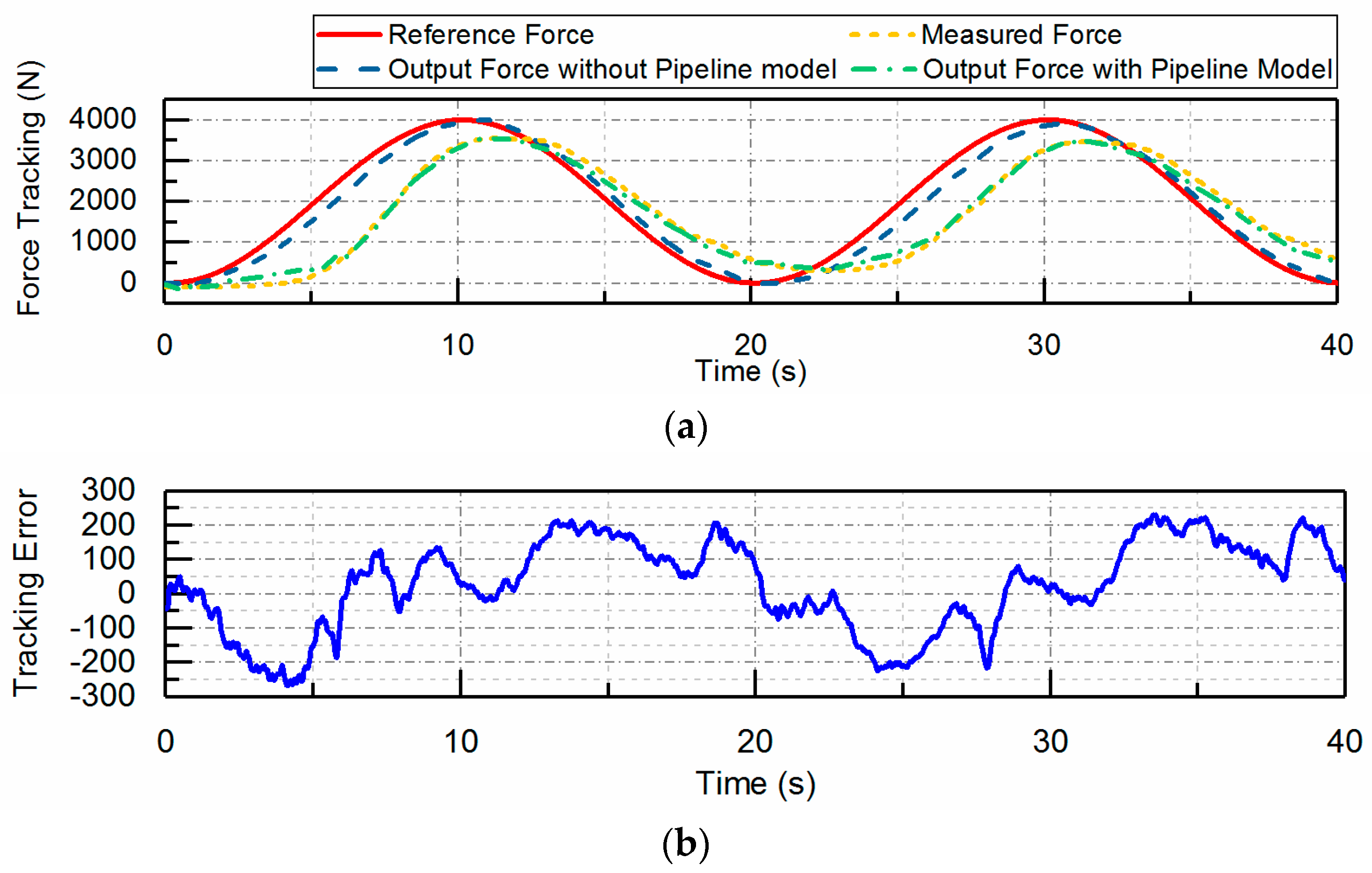
5.4.2. Case II: Sine Wave

In the first case, to further verify the force control performance of the proposed EFABC, a sine wave force was utilized, which was smooth enough. Moreover, three performance indexes, including the maximum tracking error $M_e$, average tracking error $\mu$ and standard deviation of the tracking error $\sigma$, were utilized to measure the quality of each control algorithm and are summarized in

Table 4. Performance indexes with sine reference force.

Index	10 # (0 m)			32 # (4500 m)			150 # (11,000 m)
	${\mathbf{M}}_{\mathbf{e}}{}_{10}$	${\mathsf{\mu }}_{10}$	${\mathsf{\sigma }}_{10}$	${\mathbf{M}}_{\mathbf{e}}{}_{32}$	${\mathsf{\mu }}_{32}$	${\mathsf{\sigma }}_{32}$	${\mathbf{M}}_{\mathbf{e}}{}_{150}$	${\mathsf{\mu }}_{150}$	${\mathsf{\sigma }}_{150}$
PI	243.52	−1.59	103.83	613.15	−13.88	340.91	1027.30	−122.70	264.32
EABC	237.65	−86.36	133.65	1373.89	60.82	561.02	1100.31	34.49	313.21
EFABC	175.28	−115.36	147.08	430.99	37.84	200.93	525.81	−35.28	276.15

. The experimental results are presented in Figure 17, Figure 18, Figure 19, Figure 20, Figure 21 and Figure 22. As seen from Figure 17, Figure 19 and Figure 21, in the case of selecting 10# as the working medium, the maximum tracking error $M_{e10}$ of the proposed EFABC controller was 175.28 N, which was 28% lower than PI and 26.2% lower than EABC. The average tracking error ${\mu }_{10}$, and the standard deviation of the tracking error ${\sigma }_{10}$, of the proposed EFABC controller were a bit larger than the other two controllers. In the case of selecting 32# as the working medium, the maximum tracking error $M_{e32}$ of the proposed EFABC controller was 430.99 N, which was 29.7% lower than PI and 68.6% lower than EABC. The standard deviation of the tracking error ${\sigma }_{32}$ of the proposed EFABC controller was the smallest of the three controllers. In the case of selecting 150# as the working medium, the maximum tracking error $M_{e150}$ of the proposed EFABC controller was 525.81 N, which was 48.8% lower than PI and 52.2% lower than EABC. The average tracking error ${\mu }_{150}$, and the standard deviation of the tracking error ${\sigma }_{150}$, of the proposed EFABC controller were similar to the other two controllers. We can come to the conclusion that the proposed controllor had adequate tracking performance when using different oil with different viscosities as the working media; the other two controllers did not show a satisfactory performance. The estimates of velocity when working under different viscosities of oil could track the velocity obtained by the displacement differentiation well and had low noise, as shown in Figure 18, Figure 20 and Figure 22.

6. Conclusions

In this study, we developed a fuzzy adaptive backstepping control method based on an extended state observer to realize the output force control of typical joints with long transmission pipelines of deep-sea hydraulic manipulators. Unlike terrestrial environments, where force sensors are available, the proposed method uses the pressures at the servo valve port as feedback to control the output force of a deep-sea hydraulic cylinder. Using the velocity information obtained by the extended state observer and pressure information measured by pressure sensors at the servo valve port, the pressure of cylinder chambers used in the method can be estimated by the established pipeline model in real time. Parameter uncertainty in the system caused by variations in working depth is then compensated with an adaptation law. Fuzzy technology is employed to the adaptive backstepping controller to adjust the control gains to adapt to different depths. The stability of the system is guaranteed via the Lyapunov method. The proposed controller and other two controllers were implemented on an experimental system based on xPC. The comparative experimental results show that the proposed controller is effective for the force tracking of signal trajectories and has a better force control performance than std PI and EABC. We selected oils with different viscosities to simulate the working environment at different depths, focusing on the changes in viscosity with pressure, without studying the effect of density changes in detail. Thus, this issue should be considered in future work. Moreover, whether the proposed controller has better performance than intelligent control algorithms, such as reinforcement learning, needs to be further studied in the future.

References

1. Sivčev, S.; Coleman, J.; Omerdić, E.; Dooly, G.; Toal, D. Underwater manipulators: A review. Ocean. Eng. 2018, 163, 431–450. [Google Scholar] [CrossRef]
2. Zhang, Q.; Wang, H.; Li, B.; Cui, S.; Zhao, Y.; Zhu, P.; Sun, B.; Zhang, Z.; Li, Z.; Li, S. Development and Sea Trials of a 6000m Class ROV for Marine Scientific Research, 2018 OCEANS-MTS/IEEE Kobe Techno-Oceans (OTO); IEEE: New York, NY, USA, 2018; pp. 1–6. [Google Scholar]
3. Walters, R.B. Hydraulic and Electric-Hydraulic Control Systems; Springer: Berlin/Heidelberg, Germany, 2000. [Google Scholar]
4. Brennan, M.L.; Cantelas, F.; Elliott, K.; Delgado, J.P.; Bell, K.L.C.; Coleman, D.; Fundis, A.; Irion, J.; Van Tilburg, H.K.; Ballard, R.D. Telepresence-Enabled Maritime Archaeological Exploration in the Deep. J. Marit. Archaeol. 2018, 13, 97–121. [Google Scholar] [CrossRef]
5. Ruff, S.E.; Felden, J.; Gruber-Vodicka, H.R.; Marcon, Y.; Knittel, K.; Ramette, A.; Boetius, A. In situ development of a methanotrophic microbiome in deep-sea sediments. ISME J. 2019, 13, 197–213. [Google Scholar] [CrossRef] [PubMed] [Green Version]
6. Drap, P.; Seinturier, J.; Hijazi, B.; Merad, D.; Boi, J.-M.; Chemisky, B.; Seguin, E.; Long, L. The ROV 3D Project: Deep-sea underwater survey using photogrammetry: Applications for underwater archaeology. J. Comput. Cult. Herit. (JOCCH) 2015, 8, 1–24. [Google Scholar] [CrossRef]
7. Chen, Y.; Zhang, Q.; Feng, X.; Huo, L.; Tian, Q.; Du, L.; Bai, Y.; Wang, C. Development of a Full Ocean Depth Hydraulic Manipulator System, International Conference on Intelligent Robotics and Applications; Springer: Berlin/Heidelberg, Germany, 2019; pp. 250–263. [Google Scholar]
8. Mattila, J.; Siuko, M.; Vilenius, M. On Pressure/Force Control of a 3 Dof Water Hydraulic Manipulator. In Proceedings of the JFPS International Symposium on Fluid Power; The Japan Fluid Power System Society: Tokyo, Japan, 2005; pp. 443–448. [Google Scholar]
9. Linjama, M.; Huova, M. Model-based force and position tracking control of a multi-pressure hydraulic cylinder. Proc. Inst. Mech. Eng. Part I J. Syst. Control Eng. 2018, 232, 324–335. [Google Scholar] [CrossRef]
10. D’Souza, A.F.; Oldenburger, R. Dynamic response of fluid lines. J. Basic Eng. 1964, 86, 589–598. [Google Scholar] [CrossRef]
11. Stecki, J.S.; Davis, D.C. Fluid transmission lines—Distributed parameter models part 1: A review of the state of the art. Proc. Inst. Mech. Eng. Part A Power Process Eng. 1986, 200, 215–228. [Google Scholar] [CrossRef]
12. Johnston, D.N. A time-domain model of axial wave propagation in liquid-filled flexible hoses. Proc. Inst. Mech. Eng. Part I J. Syst. Control Eng. 2006, 220, 517–530. [Google Scholar] [CrossRef]
13. Yang, L.; Moan, T. Dynamic analysis of wave energy converter by incorporating the effect of hydraulic transmission lines. Ocean Eng. 2011, 38, 1849–1860. [Google Scholar] [CrossRef]
14. Watton, J. Modelling of electrohydraulic systems with transmission lines using modal approximations. Proc. Inst. Mech. Eng. Part B Manag. Eng. Manuf. 1988, 202, 153–163. [Google Scholar] [CrossRef]
15. Yang, W.; Tobler, W. Dissipative modal approximation of fluid transmission lines using linear friction model. J. Dyn. Sys. Meas. Control 1991, 113, 152–162. [Google Scholar] [CrossRef]
16. Mikota, G. Modal analysis of hydraulic pipelines. J. Sound Vib. 2013, 332, 3794–3805. [Google Scholar] [CrossRef]
17. Ayalew, B.; Kulakowski, B.T. Modeling supply and return line dynamics for an electrohydraulic actuation system. ISA Trans. 2005, 44, 329–343. [Google Scholar] [CrossRef]
18. Shen, G.; Zhu, Z.-C.; Li, X.; Tang, Y.; Hou, D.-D.; Teng, W.-X. Real-time electro-hydraulic hybrid system for structural testing subjected to vibration and force loading. Mechatronics 2016, 33, 49–70. [Google Scholar] [CrossRef]
19. Cheng, L.; Zhu, Z.-C.; Shen, G.; Wang, S.; Li, X.; Tang, Y. Real-Time Force Tracking Control of an Electro-Hydraulic System Using a Novel Robust Adaptive Sliding Mode Controller. IEEE Access 2020, 8, 13315–13328. [Google Scholar] [CrossRef]
20. Jing, C.; Xu, H.; Jiang, J. Dynamic surface disturbance rejection control for electro-hydraulic load simulator. Mech. Syst. Signal Process. 2019, 134, 106293. [Google Scholar] [CrossRef]
21. Zang, W.; Zhang, Q.; Su, J.; Feng, L. Robust Nonlinear Control Scheme for Electro-Hydraulic Force Tracking Control with Time-Varying Output Constraint. Symmetry 2021, 13, 2074. [Google Scholar] [CrossRef]
22. Yuan, H.-B.; Na, H.-C.; Kim, Y.-B. Robust MPC–PIC force control for an electro-hydraulic servo system with pure compressive elastic load. Control Eng. Pract. 2018, 79, 170–184. [Google Scholar] [CrossRef]
23. Nakkarat, P.; Kuntanapreeda, S. Observer-based backstepping force control of an electrohydraulic actuator. Control Eng. Pract. 2009, 17, 895–902. [Google Scholar] [CrossRef]
24. Li, X.; Zhu, Z.-C.; Rui, G.-C.; Cheng, D.; Shen, G.; Tang, Y. Force Loading Tracking Control of an Electro-Hydraulic Actuator Based on a Nonlinear Adaptive Fuzzy Backstepping Control Scheme. Symmetry 2018, 10, 155. [Google Scholar] [CrossRef]
25. Wang, C.; Jiao, Z.; Wu, S.; Shang, Y.J.M. Nonlinear adaptive torque control of electro-hydraulic load system with external active motion disturbance. Mechatronics 2014, 24, 32–40. [Google Scholar] [CrossRef]
26. Guo, Q.; Zhang, Y.; Celler, B.G.; Su, S.W. Backstepping Control of Electro-Hydraulic System Based on Extended-State-Observer With Plant Dynamics Largely Unknown. IEEE Trans. Ind. Electron. 2016, 63, 6909–6920. [Google Scholar] [CrossRef]
27. Yao, J.; Jiao, Z.; Ma, D. Extended-State-Observer-Based Output Feedback Nonlinear Robust Control of Hydraulic Systems With Backstepping. IEEE Trans. Ind. Electron. 2014, 61, 6285–6293. [Google Scholar] [CrossRef]
28. Zhang, Z.; Duan, G.; Hou, M. Applications, Robust adaptive dynamic surface control of uncertain non-linear systems with output constraints. IET Control Theory Appl. 2017, 11, 110–121. [Google Scholar] [CrossRef]
29. Guo, Q.; Liu, Y.; Jiang, D.; Wang, Q.; Xiong, W.; Liu, J.; Li, X. Prescribed Performance Constraint Regulation of Electrohydraulic Control Based on Backstepping with Dynamic Surface. Appl. Sci. 2018, 8, 76. [Google Scholar] [CrossRef] [Green Version]
30. Sa, Y.; Zhu, Z.; Tang, Y.; Li, X.; Shen, G. Adaptive dynamic surface control using nonlinear disturbance observers for position tracking of electro-hydraulic servo systems. Proc. Inst. Mech. Eng. Part I J. Syst. Control Eng. Pract. 2022, 236, 634–653. [Google Scholar] [CrossRef]
31. Ahn, K.K.; Truong, D.Q. Online tuning fuzzy PID controller using robust extended Kalman filter. J. Process Control 2009, 19, 1011–1023. [Google Scholar] [CrossRef]
32. Truong, D.Q.; Ahn, K.K. Force control for hydraulic load simulator using self-tuning grey predictor—Fuzzy PID. Mechatronics 2009, 19, 233–246. [Google Scholar] [CrossRef]
33. Cerman, O.; Hušek, P. Adaptive fuzzy sliding mode control for electro-hydraulic servo mechanism. Expert Syst. Appl. 2012, 39, 10269–10277. [Google Scholar] [CrossRef]
34. Chen, Y.; Zhang, Q.; Tian, Q.; Huo, L.; Feng, X. Fuzzy Adaptive Impedance Control for Deep-Sea Hydraulic Manipulator Grasping Under Uncertainties. In Global Oceans 2020: Singapore—U.S. Gulf Coast; IEEE: New York, NY, USA, 2020; pp. 1–6. [Google Scholar]
35. Goodson, R.; Leonard, R. A survey of modeling techniques for fluid line transients. J. Basic Eng. 1972, 94, 474–482. [Google Scholar] [CrossRef]
36. Guo, Q.; Zhang, Y.; Celler, B.G.; Su, S.W. State-Constrained Control of Single-Rod Electrohydraulic Actuator With Parametric Uncertainty and Load Disturbance. IEEE Trans. Control Syst. Technol. 2018, 26, 2242–2249. [Google Scholar] [CrossRef]
37. Tian, Q.; Zhang, Q.; Chen, Y.; Huo, L.; Li, S.; Wang, C.; Bai, Y.; Du, L. Influence of Ambient Pressure on Performance of a Deep-sea Hydraulic Manipulator; OCEANS 2019-Marseille; IEEE: New York, NY, USA, 2019; pp. 1–6. [Google Scholar]
38. Xie, F.; Hou, Y. Oil film hydrodynamic load capacity of hydro-viscous drive with variable viscosity. Ind. Lubr. Tribol. 2011, 63, 210–215. [Google Scholar] [CrossRef]
Figure 1. Mainframe mechanical structure of a typical deep-sea hydraulic manipulator.
Jmse 10 01467 g001
Figure 2. Schematic diagram of the system.
Jmse 10 01467 g002
Figure 3. Membership functions of inputs.
Jmse 10 01467 g003
Figure 4. Membership functions of outputs: (a) output variable u 1 ; (b) output variable u 2 .
Jmse 10 01467 g004
Figure 5. Block diagram of the proposed force controller.
Jmse 10 01467 g005
Figure 6. The experiment system configuration.
Jmse 10 01467 g006
Figure 7. Schematic diagram of the experimental system: (1) Pump; (2) filter; (3) relief valve; (4) accumulator; (5) check valve; (6) solenoid valve; (7) servo valve; (8) pressure sensor; (9) pipeline; (10) hydraulic cylinder; (11) position sensor.
Jmse 10 01467 g007
Figure 8. Experimental results with 10#: (a) force tracking performance; (b) force tracking error between the force obtained by the proposed method and measured by the force sensor.
Jmse 10 01467 g008
Figure 9. Experimental results with 32#: (a) force tracking performance; (b) force tracking error between the force obtained by the proposed method and measured by the force sensor.
Jmse 10 01467 g009aJmse 10 01467 g009b
Figure 10. Experimental results with 150#: (a) force tracking performance; (b) force tracking error between the force obtained by the proposed method and measured by the force sensor.
Jmse 10 01467 g010
Figure 11. Experimental results with 10#: (a) force tracking performance; (b) force tracking error.
Jmse 10 01467 g011
Figure 12. Experimental results with 10#: estimated velocity of EFABC.
Jmse 10 01467 g012
Figure 13. Experimental results with 32#: (a) force tracking performance; (b) force tracking error.
Jmse 10 01467 g013
Figure 14. Experimental results with 32#: estimated velocity of EFABC.
Jmse 10 01467 g014
Figure 15. Experimental results with 150#: (a) force tracking performance; (b) force tracking error.
Jmse 10 01467 g015aJmse 10 01467 g015b
Figure 16. Experimental results with 150#: estimated velocity of EFABC.
Jmse 10 01467 g016
Figure 17. Experimental results with 10#: (a) force tracking performance; (b) force tracking error.
Jmse 10 01467 g017
Figure 18. Experimental results with 10#: estimated velocity of EFABC.
Jmse 10 01467 g018
Figure 19. Experimental results with 32#: (a) force tracking performance; (b) force tracking error.
Jmse 10 01467 g019
Figure 20. Experimental results with 32#: estimated velocity of EFABC.
Jmse 10 01467 g020
Figure 21. Experimental results with 150#: (a) force tracking performance; (b) force tracking error.
Jmse 10 01467 g021
Figure 22. Experimental results with 150#: estimated velocity of EFABC.
Jmse 10 01467 g022