1. Introduction
In this paper, the problems of the modeling and motion control system design of barge ships are considered. Barge ships are mainly used to transport huge and heavy pieces of cargo or equipment, which is difficult for conventional ships. However, since barges are not equipped with propulsion systems and are instead towed by tugboats, it is difficult to achieve accurate and rapid motion and positioning requirements. Moreover, safety and stability cannot be guaranteed because the system operations rely heavily on the experience and skills of the operators. Recently, with the development of dynamic positioning systems (DPSs), the motion control performance of surface-type ships has been remarkably improved. In many cases, DPSs use the ships’ own propellers and thrusters. However, in the particular case of barge operation, most of this work is carried out by tugboats.
Numerous studies have been conducted on the automatic control of ship motion via DPSs using tugboats. For example, a control method for towing vessels using single tugboats has been proposed [
1,
2,
3]. These authors considered scenarios in which vessels were lost or could not use their propulsion systems, so needed towing by tugboats. However, unlike barges, the vessels in these studies were able to control their rudders to maneuver their trajectories. Additionally, barge ships are usually much larger and heavier, so the towing force from single tugboats would be insufficient and multiple tugboats with an appropriate allocation are required. For instance, the combination of two tugboats and a damper system was suggested in [
4,
5,
6] to ensure the stable and fast berthing operation of a mother ship. The tugboats pushed the ship from one side following the berthing direction, while the damper system was fixed on the harbor contacts and supported the ship from the other side. It is also worth noting that tugboats can either push or tow ships; hence, damper systems are essential for complete berthing operations, i.e., both horizontal positions and the heading angle of ships are controlled through tugboat systems. Otherwise, there must be four or more tugboats operating simultaneously to fully convey ships [
7].
DPSs using four tugboats were used for vessel berthing in [
8,
9,
10] and barge positioning in [
11]. The tugboats were arranged on four sides of the controlled ships and provided thrust in four different directions. A similar configuration was applied for a ship conveying system using five or six tugboats in [
7]. It seems to be an appropriate arrangement since the thrust can be evenly distributed and the forces and torque in the required directions are easily obtained. However, considering the working environments of barge ship conveying systems, i.e., transporting, loading and unloading heavy cargo in narrow spaces (such as shipyards), this configuration becomes inappropriate. For example, in the berthing process, tugboats adjust their thrust force appropriately so that the controlled barge ship slowly and smoothly approaches the harbor wall. Then, the berth-side tugboats are asked to move out of the ship’s path and the other tugboats, which can only push the ship toward the dock, have to work very gently resulting in a slow and inefficient berthing operation.
Figure 1 shows an example of this situation.
Some studies [
8,
9,
10,
11] have also shown that mother ships could be effectively conveyed using properly controlled thrust from tugboats, i.e., ships were able to follow a trajectory (for example, the planned route for ship berthing) or be positioned at desirable set points. Unfortunately, from a practical point of view, the demanding properties of barge motion control are still not easily achieved. One of the main reasons for this is that so far, all control actions, i.e., the operation of tugboats, have been performed manually, so the control performance depends entirely on the competence and experience of the operators. The control performance focuses on the stability of the process rather than speed. Additionally, the propulsion systems of tugboats still rely on internal combustion engines, which makes it challenging to adopt automatic control systems for autonomous operations. Fortunately, electric and self-propelled/remote-controlled tugboats have recently been developed. Fully electric tugboats have even reached the commercial stage [
12]. This has opened up the opportunity to dramatically improve DPS operations using tugboats.
Therefore, in this study, we developed a control system for tugboats that could quickly and safely convey barge ships along the desired path to the target position within the working environments of the barges. To achieve this objective, we first developed a novel configuration using four tugboats to convey barge ships. Then, we formulated a dynamic model of a barge, incorporating the assembly of the four tugboats. To this end, we designed a sliding mode controller to achieve the robust stability and desired performance of barge motion. Sliding mode controllers offer robust control techniques that can cope with uncertainties and disturbances in water environments, as in [
9,
10], while simultaneously achieving control performance. Control systems operate the thrust/towing forces of tugboats so that barges can follow desired trajectories and be positioned at the required set points with only small errors, even in harsh environments. We also introduced an
controller, which are well known for preserving the robustness of control systems, for the sake of comparison. We also conducted simulation studies to validate the efficiency of the proposed configuration and control system.
2. Proposed Configuration and System Modeling
2.1. Proposed Configuration
This study considered a barge ship as the mother ship and developed a conveying system using four tugboats. The barge ship did not have a propulsion system and could only move with the assistance of the tugboats. We considered the narrow working space of the barge and other special operations, such as berthing. These operations made the tugboat configurations from previous studies inappropriate. Therefore, we deemed it reasonable to place all of the tugboats on one side of the barge, for example, on the outboard side of the barge during berthing operations. Then, for complete control of the barge’s translation and rotation, two pairs of tugboats operated in opposite directions: two tugboats towed the barge, while the other two pushed it.
A schematic drawing of the proposed configuration is depicted in
Figure 2 [
13]. The system consisted of the barge’s body-fixed frame (
) and a reference Earth-fixed frame. The parameters of the configuration presented in
Figure 2 can be summarized as follows:
represent the heading angle of the barge ship and tugboats;
represents the angle between the axis and the line from the barge’s center to the ith connection point of the conveying system;
represents the angle between the axis and the ith control force;
represents the angle between the axis and the ith control force;
represents the angle of the rudder of the ith tugboat;
represents the length of the rope from the connection on the barge ship to the ith tugboat;
represents the distance from the center of the barge to the ith connection/contact point of the conveying system;
represents the longitudinal distance from the center of the barge to the connection/contact points of the conveying system;
represents the lateral distance from the center of the barge to the connection/contact points of the conveying system.
denotes the forces generated by the tugboats. In detail, and represent the pulling forces from the two outboard tugboats pulling the barge using ropes and and represent the pushing forces from the other two tugboats. represents the propulsion force and denotes the reaction of the towing force acting on the ith tugboat. The forces and torque of the tugboats were generated by their main propellers and aft rudders. The dynamics of the tugboats that pushed the mother ship in this proposed configuration were identical to those in conventional arrangements and have been well studied in previous publications. Moreover, we could just consider their forces acting on the barge and dismiss their dynamics within the total system. Hence, only the motion of the barge ship and the tugboats were derived in this study. To examine the controllability of the proposed configuration, as well as to then design a control system, the planar dynamics of the barge and the towing tugboats were derived.
2.2. Barge Ship Modeling
For the sake of simplicity, the barge ship was assumed to be symmetric in the planar plane and its center of gravity was assumed to coincide with the origin of the body-fixed frame. Then, the motion equation of the barge ship could be represented in the following form [
14]:
where
denotes the inertia matrix (which included the mass
, the moment of inertia about the
axis of the barge
, the added mass
and the added inertia
) and
is the damping matrix.
and
were described as follows [
14]:
was used to represent the position and the heading angle of the barge in the Earth-fixed frame.
was used to represent the surge, sway and yaw rates in the body-fixed frame.
was the rotation matrix between the Earth-fixed frame and the body-fixed frame, which was defined as follows [
14]:
The force and moment vector
represented the surge force, sway force and yaw moment. They could be derived using the configuration matrix
of the conveying system in
Figure 2 as follows:
where
and
. The amplitude of the force was positive for towing and negative for pushing.
was the control force vector that was generated by the four tugboats as an actuator. A control allocation was required to compute the force from each tugboat for the required force and moment vector
of the barge. One of the common methods for this is based on the Moore–Penrose pseudoinverse
of the configuration matrix
, i.e.,:
In other words, given the angles
, the corresponding control force
could be calculated. Moreover, the following relationship between the
and
could be written from Equation (1):
Then, the motion equation could be written solely in the Earth-fixed frame as follows [
14]:
where the system matrices
,
and
were given by:
was the skew-symmetric matrix of the rotation, which was defined as follows:
2.3. Towing Tugboat Modeling
In the same manner, the state
represented the position and heading angle of tugboat 1 within the Earth-fixed frame. The motion equation of tugboat 1 was written as follows [
14]:
where
is the inertia matrix and
is the damping matrix of the tugboat. The force and torque vector
was generated by the tug’s propulsion force
and towing force
.
represented the force by tug’s rudder, with
denoting the rudder angle and
denoting the vector of coefficients.
and
were defined as follows:
Equation (11) indicated that by adjusting the propulsion force, rudder angle and heading angle, the tugboat was always able to provide the required towing force
for the barge ship, as well as the force and torque
that were required for its own motion. Moreover, as shown in
Figure 2, the tugboat’s position could be represented as follows:
Substituting Equation (12) and the relationship
into Equation (10), the motion equation of tugboat 1 could be rewritten as follows:
where
and
In the same manner, the motion equation of tugboat 2 was derived as:
where
is the inertia matrix and
is the damping matrix. The position of tugboat 2
was represented in terms of the barge ship’s position and heading angle by:
Consequently, Equation (16) could be rewritten as follows:
where
The motion equation of the entire system shown in
Figure 2 could be represented by combining the resulting motion equations of the barge ship and tugboats. By defining the new state vector
and control input vector
, the model of the system was given by:
where the system matrices were defined as follows:
3. Control System Design
Then, we designed a control system to move the barge ship, which did not have a propulsion system, to the desired position safely and quickly, i.e., the objective of the control system was to operate the tugboats such that the robust route tracking and positioning performance of the barge ship was ensured, even in the presence of disturbances. It is worth noting that the towing forces from the tugboats only acted on the barge when the ropes were in tension. Therefore, the position and orientation of the towing tugboats needed to be controlled. Their desired trajectories were obtained from those of the barge and Equations (11) and (17). Considering the uncertainties and disturbances in the application, we needed to design the control system based on robust control design frameworks. A sliding mode controller was developed and an controller was introduced for the sake of comparison.
3.1. Sliding Mode Control Design
The proposed sliding mode control input was defined by a summation of the equivalent control part
and the switching control part
, i.e.,:
The sliding surface was defined as follows:
where
is the controller gain matrix, which was diagonal positive definite.
was the tracking error, where
is the state vector that was defined in the previous section and
is the vector for the corresponding desired position and orientation. All of these were expressed in the Earth-fixed frame. The convergence of the sliding surface to zero implied that the state error
converged to zero. We defined a virtual state error in the Earth-fixed frame as follows:
Then, from Equations (23) and (24), the sliding surface could be rewritten as follows:
Using the sliding surface in Equation (25), the entire system in Equation (20) could be derived as:
By letting
, the equivalent control could be obtained as follows:
In order to guarantee that the sliding surface converged to zero in a finite time, we introduced a sliding surface dynamic with the following expression:
where
and
are diagonal positive definite controller gain matrices and
denotes the signum function. The following switching part of the control law was chosen to ensure the introduced dynamics:
The following non-negative Lyapunov function was chosen to verify the stability of the system:
Hence, the time derivative of
, using the control input given in Equations (27) and (29), was obtained as follows:
Therefore, we could conclude that the control system was asymptotically stable.
In Equation (29), the discontinuous signum function could generate the chattering phenomenon in a neighborhood of the sliding surface
. Hence, to reduce the phenomenon, the signum function was replaced by the saturation function in Equation (32):
where
is the thickness of the boundary layer [
15]. Then, the resulting control input was obtained as follows:
3.2. Controller Design
An
controller was introduced to compare the control performance of the proposed controller. The
method is one of the most preferred control techniques for acting on uncertainties [
16]. The standard configuration of a control system is shown in
Figure 3.
In
Figure 3,
represents the external input,
denotes the output signals and
is the generalized plant of the proposed system. We defined the closed-loop transfer function from
to
as
. The objective of the
controller design was to find
, such that the
norm of the closed-loop transfer function was less than a given positive number (
), as shown following equation:
On the other hand, when
and
were sufficiently small, we could obtain a linear state-space model that represented the dynamic characteristics of the entire system. This was achieved by defining the new state vector
and the control input vector
. The state-space model was represented as follows:
where the system matrices were given by:
with
Referring back to the problem in Equation (34), we could obtain the generalized plant
regarding the state-space model in Equation (35) by letting
and
.
represented the desired value of the state
. The plant
in the mixed sensitivity
control framework is presented in Equation (38) and illustrated in
Figure 4.
The controller could be derived simply using MATLAB software with the state-space model that was presented in Equations (35) and (38).
4. Simulations
Simulation studies were conducted for two scenarios to show the usefulness of the proposed system. The first scenario was a two-set point tracking, in which the barge ship needed to move from its initial position to two consecutive set points. In the second simulation, the barge was required to follow a desired quarter-circle trajectory. Both scenarios were designed similarly, according to the motion of the ship during berthing. In addition, the motion control performance in each scenario was verified with and without the presence of disturbances.
The ship models that were used in the simulations were scale models that have been presented in previous experimental studies [
2,
3,
17]. Their specifications are shown in
Table 1.
The inertia matrix and damping matrix of the barge ship and tugboat were listed as follows:
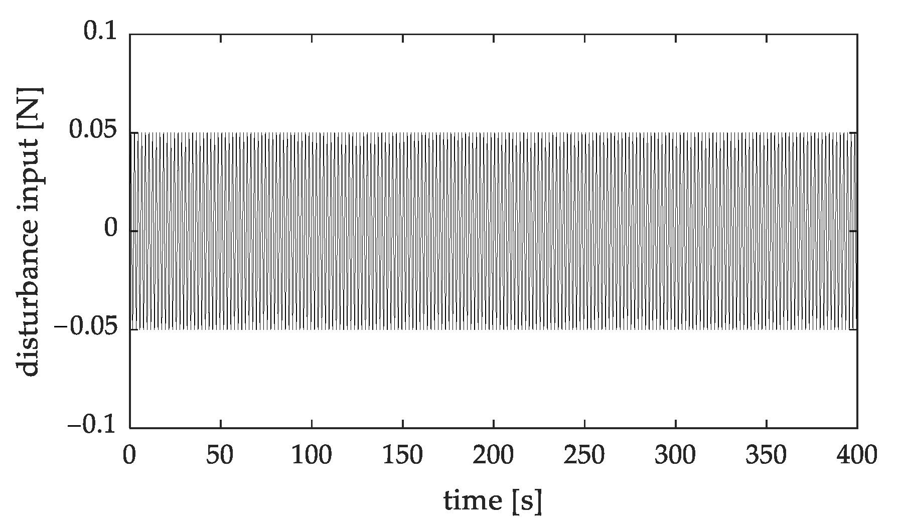
Equation (39) represented the inertia matrix and the damping matrix of the barge ship and Equation (40) represented those of the towing tugboats. In particular, tugboats 1 and 2 were assumed to have the same dynamic characteristics. The disturbance signal that was applied in the simulations was a sinusoidal signal with a magnitude
, which corresponded to
of the maximum control force
that was required for the barge ship, and a frequency
, as shown in
Figure 5.
4.1. Set Point Tracking Simulation Results
In the first scenario, the barge needed to move from its initial zero position to the first set point at
,
and
. Then, after 200 s, it headed to the second set point at
and
and, at the same time, it rotated
about its vertical axis. Thus, in the simulation, the desired values of the vector
were given by:
The tugboats also needed to move in the same manner from their initial positions at , , , , and .
Figure 6 shows the set point tracking simulation results and
Figure 7 shows the control inputs of the barge ship. The left-hand figures present the results from the
controller and the right-hand figures present those from our sliding mode controller. The results presented in
Figure 6a,b were obtained without any disturbances while
Figure 6c,d were obtained under disturbance.
Figure 6a,b show that the barge ship moved to the target position and orientation without any significant errors. Both control systems provided a good tracking performance with a feasible control input. However, during the approach phase from the first set point to the second set point, there was a tendency to deviate from the desired tracking route. This was due to the rotation of the barge ship during this period. Furthermore, using our sliding mode controller, the barge ship was able to approach the target position faster than when it was controlled by the
controller. Additionally, the barge ship deviated from the desired route due to the influence of disturbances, as seen in
Figure 6c,d. Even so, our sliding mode controller achieved a better and more robust control performance. In addition, in steady state, both controllers effectively rejected any disturbances.
4.2. Trajectory Tracking Simulation Results
In the second simulation, the desired trajectory was defined as an arc with a radius of
and an angle of 90 deg, starting from
,
and
and returning to the zero position. The initial positions of the tugboats were
,
,
,
,
and
. The trajectory ended at 400 s, then stayed still at the final position until 600 s (
Figure 8).
Figure 9 and
Figure 10 show the trajectory tracking performance and the control inputs of the barge ship. The arrangement of the figures is similar to the figures. It can easily be seen that our sliding mode controller achieved a better performance and robustness, even in the presence of disturbances. Furthermore, at the departure stage and under the influence of disturbances, the barge ship that controlled by the
controller appeared to deviate from the desired trajectory (
Figure 9c). In conclusion, the proposed conveying system using our sliding mode controller could achieve a robust motion control performance for the barge ship and thus, ensure fast and safe working operations.
5. Conclusions
In this paper, the problem of the modeling and motion control system design of conveying systems for non-propulsion barge ships was considered. Considering the narrow workspaces of barges, a new configuration for conveying systems was proposed, comprising a combination of pushing and towing tugboats that were arranged on one side of a barge. A dynamical model of the entire system was derived and showed its feasibility. Then, a motion control system based on the sliding mode framework and a comparative control system were designed to convey a barge ship safely and quickly. The control laws were obtained for the whole conveying system and, therefore, guaranteed the efficient performance of both the barge ship and the tugboats simultaneously.
To show the effectiveness of the proposed system, simulation studies were conducted. Set point tracking and trajectory tracking scenarios were considered in the simulations. From their results, the maneuverability of the proposed barge ship control configuration was validated. The proposed sliding mode controller showed its superiority over the comparative controller, especially in terms of robustness against disturbances.
However, the correlations between the trajectories of barge ships and those of tugboats have not yet been explicitly determined. This will be considered in our next study, along with more advanced control system designs. Moreover, the proposed system configuration and control system will be evaluated through further experiments. We hope that the proposed idea could help researchers to find solutions for the autonomous berthing problem.


