Influence of Stratification and Bottom Boundary Layer on the Classical Ekman Model

Abstract

A depth understanding of the different processes of water movements produced by the wind surface stress yields a better description and improvement of the marine food chain and ecosystem. The classical Ekman model proposes a hypothetical ocean, excluding the influence of continents and the Coriolis force. It also assumes infinite depth and a constant vertical eddy viscosity. The current study aims to understand how the vertical velocity profile is affected by the variation of the eddy viscosity coefficient (k_z) and the consideration of a finite depth. The study uses an ideal analytical model with the Ekman classical model as a starting point. It has been demonstrated that, for a very stratified profile, when the depth is not considered infinity, the Ekman transport tends to a direction smaller than 80°. It differs from the classical Ekman model, which proposes an approximated angle equal to 90°. Considering the modified model, it was also found that the surface current deviation is smaller than 40°, which differs from the 45° proposed by the classical model. In addition, it was determined that for ocean depths smaller than 180 m, the maximum velocity does not occur at the water surface, as in the classical model, but at deeper levels.

1. Introduction

For years, the study of Ekman transport has been carried out in a simplified manner. Simplifications and assumptions can always give approximate solutions but are not the most adequate. To correctly describe the behavior of the water bodies and all the related implications, it is essential to develop an appropriate model with the minimum of assumptions. The mentioned results can be achieved with a modified Ekman model in which stratification and turbulent viscosity variability can be considered. In addition, knowing velocities’ behavior in the ocean boundary layer is essential to answer many practical and scientific questions, from the distribution of planktonic organisms to issues related to global ocean circulation [1].

The classical Ekman model considers a balance of forces between friction and the Coriolis force to study currents driven by wind [2,3]. In a hypothetical ocean with a constant turbulent viscosity throughout the water column, Ekman deduced that the wind-driven current in the surface boundary layer decreases exponentially with depth and that the direction of the surface current deviates 45° to the right in the northern hemisphere and to the left in the southern hemisphere.

In a water column, the friction layer generated by the wind is called the Ekman layer. The wind’s physical effects along the Ekman layer involve only the friction effects due to the turbulent viscosity and the Coriolis force without considering other aspects, such as the variation of the turbulent viscosity or deeper ocean waters. This model indicates that the velocity at the surface is more significant than at any other region along the water column.

The deflection angle, defined in the classical Ekman model, increases with depth following the theoretical current pattern forming a spiral [2]. The current that passes through an imaginary vertical plane is determined as the integral of the spiral’s U and V components of the velocity vectors. This is the so-called Ekman transport, perpendicular to the wind surface direction [4,5]. As is widely known, the transport of water masses generated by continuous wind action is fundamental for the dynamics and coastal ecosystem preservation. When surface water bodies are displaced away from the coast, they are replaced by the upwelling of deep waters, i.e., below the Ekman layer, which are rich in nutrients [6,7]. The upwelling process for the southern hemisphere is described schematically in Figure 1a.

The opposite effect, sinks or downwelling, occurs when the water is transported towards the coast [8], as shown in Figure 1b. The mentioned processes facilitate the deep ocean’s oxygenation by transporting dissolved oxygen from the surface throughout the water column. Vertical movements are essential for biological productivity in the sea and therefore contribute directly to conserving the marine ecosystem [9,10].

Ekman’s simple model has been widely used to describe various ocean phenomena. A predictive study of the displacement of a thermocline in the tropical Pacific has been developed by De Witt and Leetmaa [11]. In another study by Woods and Strass, the ocean’s response to solar warming was analyzed considering the current governed by the wind [12]. Even the effects of the wind on energy generation have been analyzed considering the classical Ekman model [13]. However, few works in the literature have evaluated the impact of variable turbulent viscosity (k_z) and finite depth on the Ekman transport.

The movement between the upper layer and the underlying layers of the water column responds to the impulse exerted by the wind on the oceans and mixing processes that facilitate or not the interaction between the adjacent layers. The stratification, the superficial boundary layer, and the bottom boundary layer are three critical parameters to consider when studying the movement of water bodies [14].

Stratification is a characteristic that considers the density of water. Therefore, it is directly related to the ability to exchange physical or chemical properties between the different layers of a water column. In addition, changes in temperature at the ocean surface and differences in salt concentration (salinity) impact the stratification of the column of water [15]. Greater stratification implies a slower ocean and, therefore, has a lower mixing capacity. The mentioned characteristics directly impact the marine trophic chains and the constitution of ecosystems. A recently published study shows that, during the last sixty years, i.e., from 1960 to 2018, the global stratification of the oceans has increased 5.3%, representing an increment of around 0.90% per decade [16].

On the other hand, the bottom boundary layer is characterized by high vorticity caused by vertical gradient velocities. In the bottom boundary layer, the transport mechanisms of mixtures and sediments in coastal areas are mainly influenced by hydrodynamic processes. The study of hydrodynamic processes is also relevant when the water masses’ movement has to be described.

Therefore, the current work aims to evaluate the importance of considering stratification when the Ekman spiral is determined. An analysis taking into account a finite depth model is also added to evaluate horizontal currents in the water column by assessing their effects on the Ekman transport. The specific objectives can be expressed as follows:

• Numerically solve the equations of the classical Ekman model considering the turbulent viscosity coefficient as a function of depth and boundary conditions.
• Development of a layered profile for turbulent viscosity coefficient.
• Determine the deviation of the surface current of the modified Ekman model spiral.
• Determine the transport deviation for Ekman’s modified model.
• Contrast the velocity profile for the classic and modified Ekman model.

The rest of the paper is divided as follows: a detailed description of the modification implemented, i.e., boundary conditions and turbulent viscosity variation, to the traditional Ekman model is presented in Section 2. Section 3 presents the results with the respective discussion considering all the variations implemented in the modified Ekman model. Finally, conclusions are detailed in Section 4.

2. Materials and Methods

2.1. Ekman Modified Model

The momentum equations for the x and z components are solved using numerical methods for a turbulent, homogeneous, and inhomogeneous boundary layer in a finite water column at a steady state.

Applying the reference system indicated in Figure 2 and considering the non-slip boundary at the bottom, the following equations are solved:

$$fv+k_z\left(z\right)\frac{{\partial }^{2}u}{\partial z^2}=0$$

(1)

$$-fu+k_z\left(z\right)\frac{{\partial }^{2}v}{\partial z^2}=0$$

(2)

where f is the Coriolis parameter determined as $f=2\Omega \sin \phi$, considering the rate of the earth’s rotation $\Omega =7.292\times {10}^{-5} \mathrm{rad}/\mathrm{s}$, and φ is the latitude of the analyzed location. The solution is obtained by taking the positive z-axis upwards with z = 0 on the surface. The turbulent viscosity is expressed by k_z, which in the current study varies with the depth. The horizontal velocity components are represented by u and v (u positive towards the east and v positive towards the north).

The ocean model described in this study is fully developed using ordinary differential equations techniques with their corresponding boundary conditions. At the surface, i.e., z = 0, the driving force is given by the wind shear stress:

$${\rho }_w{k}_z{\frac{\partial u}{\partial z}|}_{z=0}={\tau }_x$$

(3)

where ${\rho }_w$ is the water density, and ${\tau }_x$ can also be computed as air density times the drag coefficient times the wind velocity component in the x-direction, i.e., ${\tau }_x={\rho }_a{C}_D{w}_x$. The shear stress in the y-direction is determined by ${\tau }_y={\rho }_a{C}_D{w}_{y,}$ where w_y is the wind velocity vector in the y-direction. The following expression is used to equal the shear stress in the y-direction:

$${\rho }_w{k}_z{\frac{\partial v}{\partial z}|}_{z=0}={\tau }_y$$

(4)

At the bottom, the non-slip boundary condition is applied, i.e., the velocity vector is equal to zero when z = −h. The following equations represent the bottom boundary condition:

$$u\left(-h\right)=0$$

(5)

$$v\left(-h\right)=0$$

(6)

The solution for the differential Equations (1) and (2) were approximated using the centered finite difference method, yielding the following correlations:

$$k_{i+1}{u}_{i+1}-2k_i{u}_i+k_{i-1}{u}_{i-1}+f{v}_i\Delta z^2=0$$

(7)

$$k_{i+1}{v}_{i+1}-2k_i{v}_i+k_{i-1}{v}_{i-1}+f{u}_i\Delta z^2=0$$

(8)

where k_i represents the turbulent viscosity coefficient for the ith layer of the discretized domain. In all the layers, the velocity components are determined as u_i and v_i for the wind velocity in the x- and y-direction, respectively. The iterative parameter i goes from 0 to n − 1 in steps of the unity, i.e., $i$ = 0,1,2,3… ($n-1$). Finally, $\Delta z$ represents the distance-step towards the depth (−h) at which the development of the discretized difference equation is evaluated.

It is also required to discretize the correlations that correspond to the boundary conditions. Once Equations (3) and (4) are discretized, they can be expressed as follows:

$${\rho }_w{k}_0\left(\frac{u_0-u_1}{\Delta z}\right)={\tau }_x$$

(9)

$$\left(\frac{{\tau }_x\Delta z}{{\rho }_w{k}_0}\right)+u_1=u_0$$

(10)

where u₀ and u₁ are the x-direction wind velocity for the first and second iterative positions, respectively. A similar process is followed for the y-components, yielding the following expressions:

$${\rho }_w{k}_0\left(\frac{v_0-v_1}{\Delta z}\right)={\tau }_y$$

(11)

$$\left(\frac{{\tau }_y\Delta z}{{\rho }_w{k}_0}\right)+v_1=v_0$$

(12)

Because the results of velocity components for the surface layer (i = 0) and bottom layer (i = n − 1) are given by applying Equations (10) and (12) to the boundary conditions represented by Equations (7) and (8), the iterative process is carried out from i = 1 to i = n − 2. Replacing i = 1 into the discretized equation gives as result the following correlations:

$$k_2{u}_2+u_1\left(k_0-2k_1\right)+f\Delta z^2{v}_1={\tau }_x\frac{\Delta z}{\rho }$$

(13)

$$k_2{u}_2+v_1\left(k_0-2k_1\right)+f\Delta z^2{u}_1={\tau }_y\frac{\Delta z}{\rho }$$

(14)

Similarly, when i = n − 2, the discretized equations are obtained as follows:

$$-2k_{n-2}{u}_{n-2}+k_{n-3}{u}_{n-3}+f{v}_{n-2}\Delta z^2=0$$

(15)

$$-2k_{n-2}{v}_{n-2}+k_{n-3}{v}_{n-3}+f{u}_{n-2}\Delta z^2=0$$

(16)

The system of equations for all the iterations comprises the matrix of coefficients, M, components u_i, and v_i of current velocity in the water column, V, and the resultant matrix, B, as shown in Figure 3.

2.2. Eddy Viscosity Coefficient

Although the classical Ekman model considers the turbulent viscosity coefficient k_z as a constant, in this study, it is expressed as a function of the depth levels where changes in its profile and the value of k_z on the surface occur. The degree of mixing turbulence, i.e., the magnitude of the turbulent viscosity, depends on how well stratified the water column is. If the water column is considered highly stratified, i.e., homogeneous, the density varies little with depth, favoring interlayer interlocking that results in mixing by turbulence. On the other hand, if the water column is stratified, i.e., composed of several bodies of water, the density changes abruptly with depth, and the mixing by turbulence is shallow or suppressed.

In Figure 4, the turbulent viscosity profiles k_z are observed. Several analyses were carried out on the modified Ekman model to evaluate the classical theory of a hypothetical ocean of constant turbulent viscosity coefficient in the water column and infinite depth. For this study, from different surface values: k_zo1 = 0.001 m²/s, k_zo2 = 0.01 m²/s, and k_zo3 = 0.1 m²/s were established for k_z in (z = 0) based on the range indicated in [17]. The profiles represented by consecutive dots correspond to a stratified water column, while those represented by dashed lines correspond to a more homogeneous water column profile.

For this study, the ocean was divided into two sections: the upper part defined from the surface at z₀ (z = 0), passing through the depth, −z_m, at which the maximum value of k_z is found, up to −z_h, which is the depth at which the values of the function of the turbulent viscosity coefficient k_z present a change of concavity in the curve or point of inflection to asymptotically approaching zero. The lower part is determined from −z_h to z = −h, as observed in Figure 5. It is clearly identified that the behavior of the coefficient k_z is directly influenced by the analyzed region.

Considering the system of equations proposed by Chen et al. [18], the following correlations allow the computation of the turbulent viscosity coefficient:

$$0\le z\le -z_h k_z=k_{z_0}\left(1-2a{z}_{m}z+a{z}^2\right)$$

(17)

$$-z_h\le z\le -h k_z=k_{z_0}e{\left|\frac{z}{z_h}\right|}^{-n}$$

(18)

where Equation (17) corresponds to Region I, while Equation (18) to Region II. In Region I, the viscosity coefficient is defined using a quadratic polynomial function. On the other hand, in Region II, the viscosity coefficient is expressed using a power function. Coefficients $a$ and $e$ are functions of the $z,$ and their position, according to Figure 5, $n$ represents the degree of the function in Region II. As a result, it is found that the k_z profile and its derivative are continuous, and they can be approximated as follows:

$$0 \le z \le -z_h a=\frac{1}{\frac{2 z_h}{n}\left(z_m-z_h\right)-z_m\left(z_h-2 z_m\right) }$$

(19)

$$-z_h \le z \le -h e=2 a \left( z_m-z_h\right) \left(\frac{z_h}{n}\right)$$

(20)

The consideration of two regions is based on the argument that the length scale for the mixture is related to the change in density in the water column. Its lower boundary layer represents the decrease of the mixture due to turbulence. The coefficient of turbulent viscosity k_z represents mixing properties due to the presence of higher density waters towards the depth [19].

As considered in the study carried out by Ianniello [20] and Cheng et al. [21], the following restrictions have been implemented:

$$\left(\mathrm{i}\right) \frac{\partial k_z}{\partial z}>0, 0 \le z \le -z_h$$

$$\left(\mathrm{ii}\right) \frac{\partial k_z}{\partial z}\le 0 -z_h \le z \le -h$$

$$\left(\mathrm{iii}\right) \frac{\partial k_z}{\partial z} \mathrm{C}\mathrm{o}\mathrm{n}\mathrm{t}\mathrm{i}\mathrm{n}\mathrm{u}\mathrm{i}\mathrm{t}\mathrm{y} \mathrm{o}\mathrm{f} \mathrm{a}\mathrm{l}\mathrm{l} z$$

The first two restrictions imply that the k_z curve in Regions I and II (see Figure 5) are increasing and decreasing, respectively. The third one asserts that k_z (−z_h) is the same in both layers, obtaining a continuous curve for the entire water column.

The proposed conditions also imply that k_z presents its maximum value in Region I or upper layers, corresponding to $k_{z m\mathrm{á}x}=k_{z_0}\left(1-a{z}_m{}^2\right)$. For this study, when a highly stratified profile is depicted, $z_m$ is established in 0.1 h while $z_h$ is set in 0.2 h. On the other hand, $z_m$ is set as 0.1 h, and $z_h$ is 0.65 h for a slightly stratified profile. In both cases, a 2nd-degree polynomial function ($n=2)$ is considered for Region II.

As mentioned, the classical Ekman model considers the equilibrium between Coriolis and the friction forces generated by wind stress. Consistent with observations of sustained ocean currents driven by the wind, its main characteristics are that the surface current deviates to the right and left of the prevailing wind direction in the northern and southern hemispheres, respectively. On the other hand, as the depth in the boundary layer increases, the current velocity is reduced. Furthermore, the direction rotates further away from the direction of the wind following a spiral. Finally, the classical model responds that the net transport is normal to the direction of the wind. The ninety degrees are measured to the right and left of the wind in the northern and southern hemispheres, respectively.

An explicit solution has been constructed for a finitely deep ocean, from 5 to 500 m (in some cases from 5 to 1000 m to visualize a trend) with depth-dependent turbulent viscosity values and a dominant wind direction of 5 m/s in the east direction ($+x$).

To compare the obtained spiral, in which the k_z profile is variable, with the classical Ekman transport, three different values of turbulence viscosity at the surface are considered: $k_{z_{0}1}=0.001 {\mathrm{m}}^2/\mathrm{s}$, $k_{z_{0}2}=0.01 {\mathrm{m}}^2/\mathrm{s}$, and $k_{z_{0}3}=0.1 {\mathrm{m}}^2/\mathrm{s}$. The differential layers along the water column are discretized in ∆z = 0.5 m. In addition, tropical, medium, and high regions are selected as 10°, 40°, and 70° latitudes, respectively. This solution covers deflection angles of the surface current from 0° to 45°. For the Ekman transport, the solutions of the deviation angles are presented from 0° to 90°. In both cases, they depend on the type of stratification.

3. Results and Discussion

3.1. Superficial Ekman Current Deviation

The variability effect of the turbulent viscosity coefficient on the deviation of the Ekman current is presented in Figure 6. The results were obtained by considering the vectors u₀ and v₀ from Equations (10) and (12). They were calculated for different finite depths, from 5 to 1000 m for highly stratified profiles and from 5 to 500 m for slightly stratified profiles. The deviations of the currents of the upper boundary layer of the spiral of the modified Ekman model are observed when the variations of k_z simulate a highly stratified water profile in Figure 6.

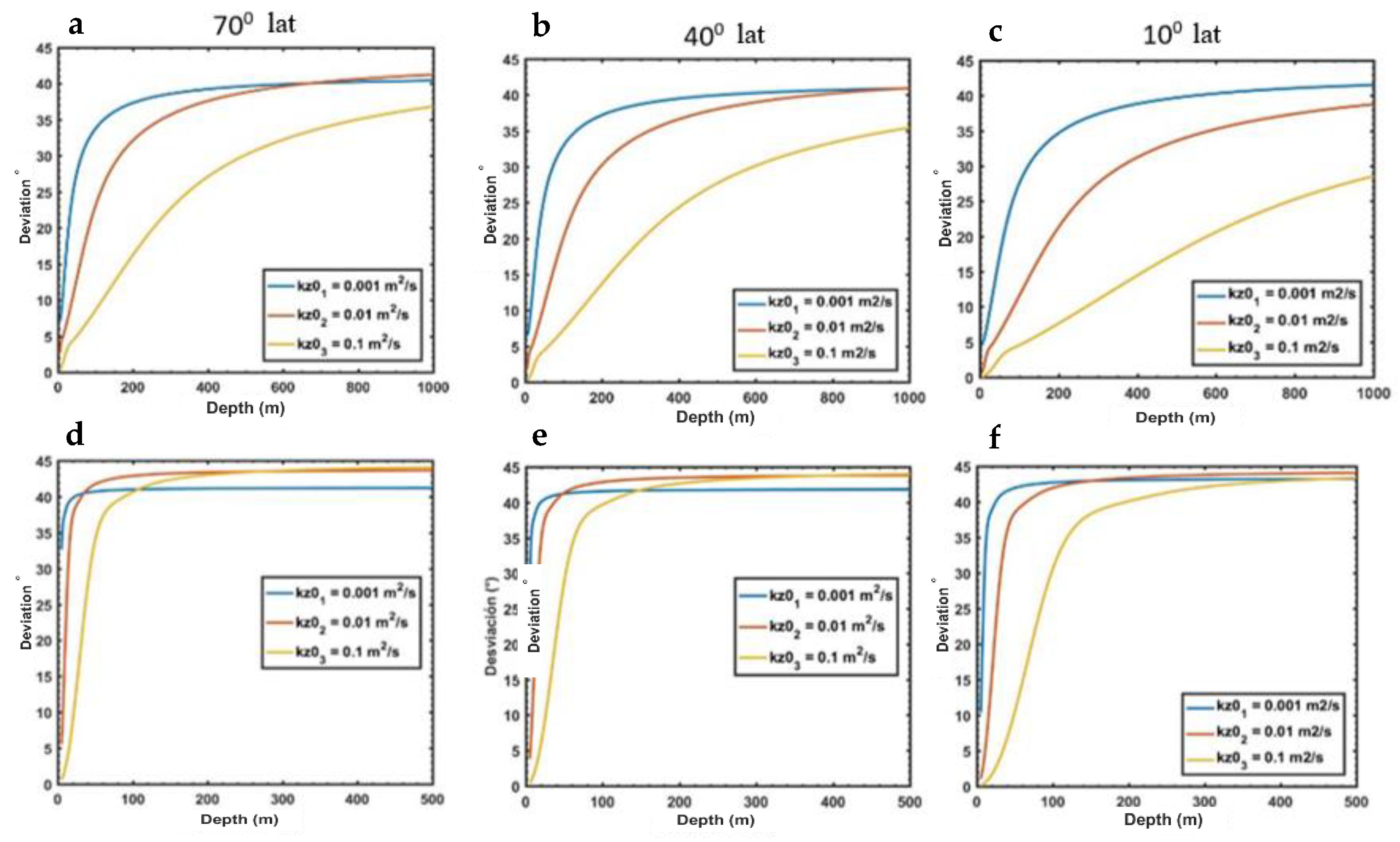
Figure 6a,b shows the results for middle and high latitudes, i.e., 70° and 40° degrees of latitude. The deviation of the surface current tends to an angle of 40° for a water column with depths close to 400 m. In addition, turbulent viscosity profiles with low values, such as k_z0 = 0.001 m²/s, were considered, and they are represented by a continuous “blue line”. For intermediate values of the turbulent viscosity profile, i.e., k_z0 = 0.01 m²/s, the trend toward 40° is observed for water columns greater than 600 m. It is represented by the “red line”.

However, for turbulent viscosity profiles with a surface value of k_z0 = 0.1 m²/s, represented by the “yellow line”, it is observed that from a depth of 800 m, the curve shows a trend smaller than 40° (towards around 35°–40°) deviation of the Ekman surface current.

In addition, Figure 6c shows the behaviors in regions close to the tropics, i.e., 10° latitude. Turbulent viscosity profile is considered with k_z0 = 0.001 m²/s (blue lines) and k_z0 = 0.01 m²/s (red line) on the surface. The trend toward 35° and 40° deviation from the surface current of the spiral is shown. It is obtained at around 600 and 800 m in depth, respectively. Meanwhile, for a turbulent viscosity profile with a viscosity at surface k_z0 = 0.1 m²/s, an increasing curve is observed towards a 30° deviation of the surface current concerning the wind velocity.

The obtained results are contrasted with the application of the modified Ekman model for slightly stratified profiles. As seen in Figure 6d–f, a 45° deviation angle from the current surface is reached with the velocity vector from the wind for 100 meters-deep water columns in the case of regions of 40° and 70° degrees of latitude. On the other hand, for tropical latitudes of 10°, the 45° deviation angle occurs in areas with a depth of 200 m, as shown in Figure 6f.

The behavior of the deviation of the surface current of the Ekman spiral for little stratification and water columns with depths greater than 200 m is similar to the classical theory [4].

Note that for latitudes of 10° and higher values of turbulent viscosity coefficient on the surface, the angle of deviation of the surface current shows a slight tendency towards smaller deviation angles of around 30°. This is shown in Figure 6c and represented by the yellow line. In contrast, for regions of greater latitude (40° lat. and 70° lat.), a more evident deviation to 40° is observed for all values of k_z0. The observed result is because, at higher latitudes, the Coriolis force diverts the water mass to a greater extent than in the tropics [22], which translates into a more active effect on the surface current, on a column of water, for a given depth.

For the analysis of shallow water columns, considered less than 100 m, and highly stratified profiles, it can be observed that in the middle and upper regions of 70° and 40° latitude, for water columns with depths of 5 to 100 m, an increasing curve is observed in the ranges 0°–7°, 2°–20°, and 7°–35° in the value of the angles of surface current deviation for turbulent viscosity coefficients. Surface values of k_z01 = 0.001 m²/s, k_z02 = 0.01 m²/s, and k_z03 = 0.1 m²/s were represented in blue, red, and yellow lines, respectively, as presented in Figure 6a,b.

For tropical latitudes of 10° (Figure 6c) and the same range of depths and profiles of turbulent viscosity coefficients on the surface, minor surface current deviations are observed in the ranges 0°–4°, 1°–7°, and 5°–30°. This indicates that the surface current vectors of the Ekman spiral are closer to the direction of the wind. This occurs because as the bottom boundary layer is near the surface, the Ekman transport is increasingly reduced because the wind shear forces predominate over the short water column. As a result, the Ekman spiral is underdeveloped.

For slightly stratified profiles, as shown in Figure 6d–f, a significant variation is observed between the angles of deviation of the surface current of the Ekman spiral of 10°, 28°, and 33° for shallow depths. It occurs in or around 5 m depth for regions of 10°, 40°, and 70° of latitude, correspondingly. The more significant deviations of this surface layer of the water column are due to the more significant influence of the Coriolis force on a profile with a lower turbulent viscosity gradient.

3.2. Ekman Transport

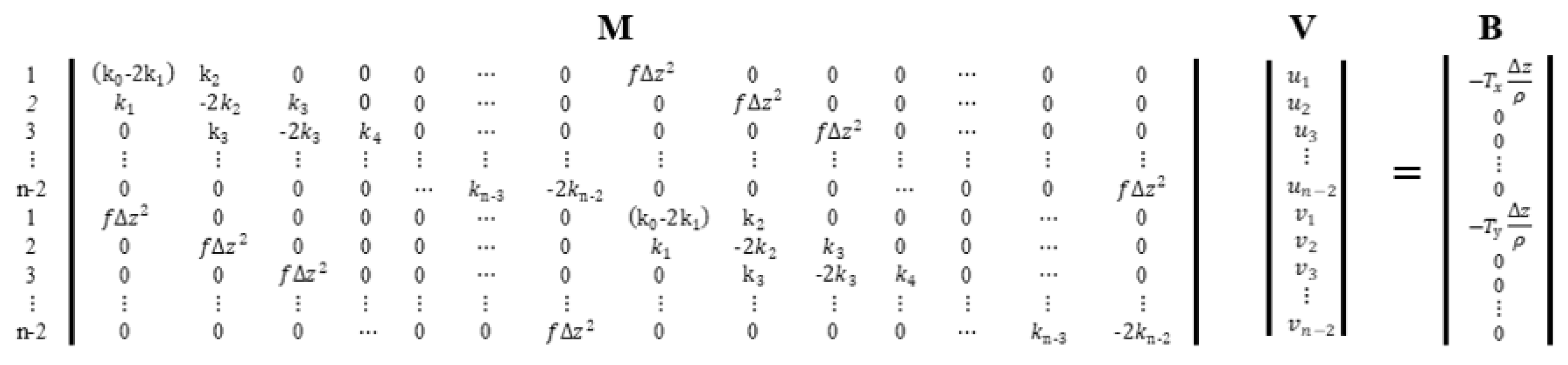
Using the turbulent viscosity coefficient profiles with their surface values k_z01, k_z02, and k_z03 described in Figure 4, a range of depths were evaluated between 5 and 1000 m (for highly stratified profiles) and between 5 and 500 m (for slightly stratified profiles). Figure 7 shows the transport results applying the modified Ekman model for the 10°, 40°, and 70° regions. From the horizontal velocity components, u and v, vertically integrated along the Ekman spiral, its resulting velocity U and V are calculated using the following expressions:

$$U=\underset{-h}{\overset{0}{\int }}u\left(z\right)dz$$

(21)

$$V=\underset{-h}{\overset{0}{\int }}v\left(z\right)dz$$

(22)

Figure 7 shows the direction, in degrees, of the Ekman transport. According to the traditional model, in a completely homogeneous ocean (k_z = constant), the average displacement of the waters occurs at 90° concerning the wind direction.

However, considering the characteristics of the current study, a non-constant turbulent viscosity profile in the water column, it is observed that with greater stratification (Figure 7a–c), the movement of the Ekman layer takes a direction towards 80° of deviation with depths greater than 200 m. In contrast, for a more homogeneous water column (Figure 7d–f), as expected, the deviation tends rapidly toward 90° for water columns greater than 200 m deep. The local maximums observed for all latitudinal regions move to the left or the shallower waters at higher latitudes (Figure 7a–c).

Comparing the results of the highly stratified water columns and the less stratified ones, it can be seen for all latitudes that the latter has the local maxima slightly more to the right or towards deeper waters. These local maxima coincide with the regions where the maximum current velocities $u$ and $v$ in the Ekman spiral occur below the ocean surface.

Results presented in Figure 8 show that for latitudes near the equator, the deviation caused by the Coriolis force influences to a lesser degree. Curves for multiple values of the turbulent viscosity coefficient k_z0 were evaluated despite keeping similar behaviors for all cases.

Unlike what would be expected in the traditional Ekman model (k_z is independent of depth), which is not the most realistic consideration due to mixing in a stable water column, the obtained result is more minor than neutral stability. The mixed layer can be thinner than the Ekman depth, and k_z will change rapidly at the bottom of the mixed layer because mixing is a function of stability. Mix generation through a stable layer is much less than mixing through a neutral stability layer.

Figure 8 shows the level, in meters below sea level, at which the maximum velocity is presented for different depths, remembering that the water column has been divided vertically into thin layers at a step of ∆z = 0.5 m.

In contrast to what is established in the classical Ekman model, where the magnitude of the velocity (speed) decreases from its maximum on the surface to lower levels in the column until it reaches zero velocity at the bottom, in the numerical development of this study, it was found that, for latitudes close to the equator (Figure 8c), and values of the turbulent viscosity coefficient on the surface k_z01 = 0.001 m²/s, k_z02 = 0.01 m²/s, and k_z03 = 0.1 m²/s, the behavior of the velocity of the Ekman spiral grows towards depths of −30, −60, and −160 m, where the maximum velocity in the spiral is close to −6, −22, and −68 m, respectively. Later, a sharp decrease in the maximum velocity is observed towards the surface. For the same values of the turbulent viscosity coefficient on the surface k_z0, the velocity of the Ekman spiral increases towards depths of −20, −50, and −80 m for 40° and 70°, as shown in Figure 8b,c. The maximum velocity in the spiral is close to −4, −12, and −38 m, for a latitude of 40°. For regions of latitude 70°, the velocity of the Ekman spiral grows towards depths from −10, −30, and −80 m, where the maximum velocity in the spiral is close to −4, −10, and −30 m, respectively. Later, a sharp decrease is observed in the maximum velocity towards the surface.

It should be noted that this behavior takes place in a highly stratified water column. Following what was previously mentioned about the turbulent viscosity profiles of Figure 4, it occurs for all latitudinal regions considered, with the fact that the further away from the tropics it is, the depth of the maximum velocities rises a few meters towards the surface.

In Figure 8, it is observed that the maximum velocity occurs below the surface at specific depths. This is observed for highly stratified profiles (see Figure 4), where the turbulent viscosity coefficient profile presents its maximum at z_m = 0.1 h. It causes, at a certain depth, more significant mixing to be generated by turbulence, i.e., greater turbulent viscosity, which then falls sharply to its inflection point at z_h = 0.2 h. It is crucial to bear in mind that the Coriolis effect is lower towards the tropics (Figure 8a), which responds that, towards these latitudes (10° latitude), the impact of wind velocity predominates over the layer. It is transmitted to consecutive layers.

In Figure 9, latitude 10° was selected with a water profile depth of 160 m and a turbulent viscosity coefficient of k_z03 = 0.1 m²/s to be analyzed. It is observed that it presents its maximum velocity at approximately 68 m at this latitude and water column depth. For this reason, Figure 9 intends to show the development of the velocities in this water column by comparing a homogeneous sea state, i.e., the classic Ekman model, with a high stratification model.

In this graph, the maximum velocity corresponds to the more considerable separation between the velocity vectors u and v, i.e., if an imaginary horizontal line is drawn, the most significant magnitude of velocity will occur at the depth at which these intersection points are most distant. Figure 9a shows the velocity profile u and v for the analytical development, with continuous blue and red lines. Purple and yellow circles represent numerical solutions for u and v velocity, respectively. The solution is obtained for an utterly homogeneous state, where the maximum velocity is presented on the surface, as the classical theory shows. In Figure 9b, in the development of a highly stratified profile, the maximum velocity occurs below the surface.

This behavior responds to the k_z profile in Figure 4. There is a very confined layer of turbulent mixing on the surface, which prevents velocity development. A velocity increases below this layer, as long as the background boundary layer is far enough to favor this result.

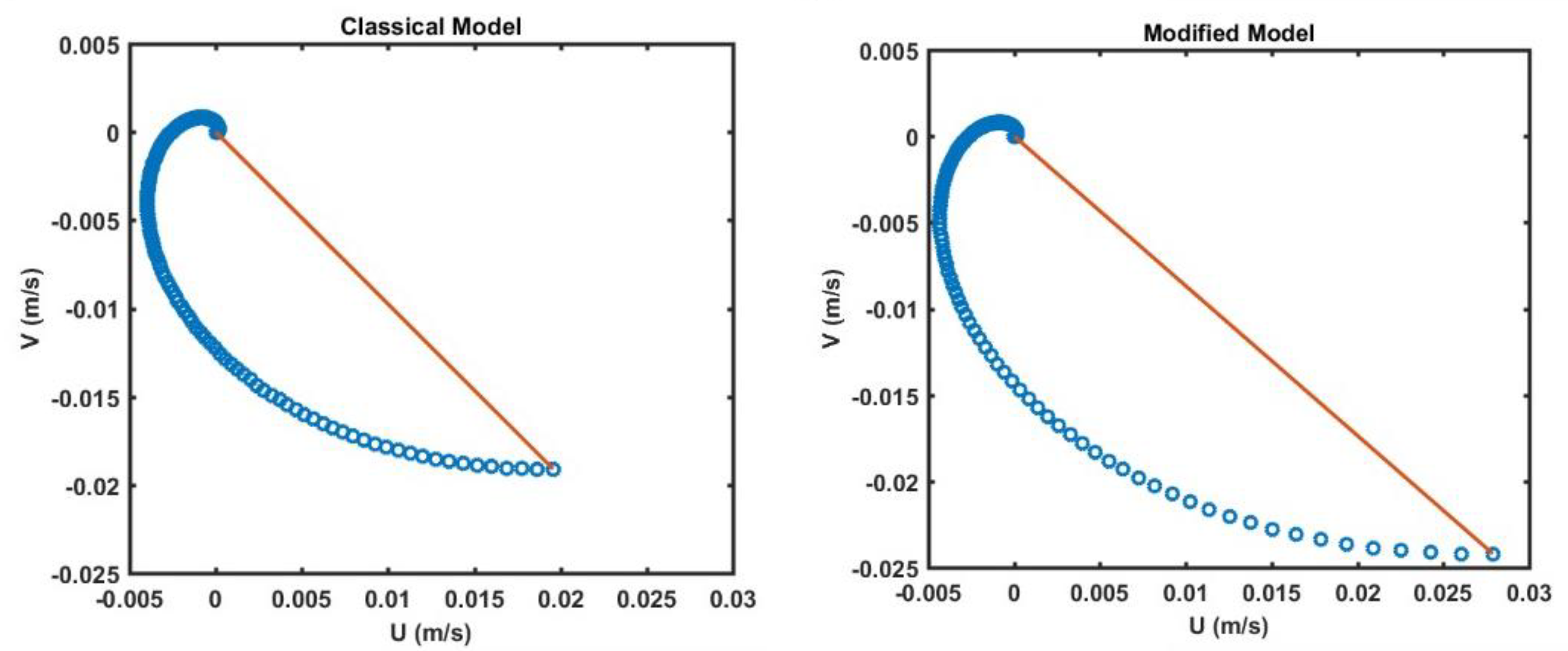
The behavior described for a latitude of 10°, in Figure 9, is similar for higher latitudes. However, the maximum velocities in the selected analysis occur in deeper waters due to the Coriolis action. Finally, Figure 10 is presented to show the difference between the Ekman spiral obtained with the classical model (left) and the modified model (right). Results are selected for a defined height of 1000 m and latitude 40°24′56.29″.

4. Conclusions

The main objective of this study was to evaluate the relative importance of stratification and a bottom boundary layer in the vertical profile of horizontal currents and deviations concerning the classic Ekman behavior. Several parameters were evaluated, such as deviation angles of the velocity of the upper boundary layer, Ekman transport, and maximum current velocity in the water column. Results were evaluated considering the variation of the turbulent viscosity k_z (z) dependent on the depth, water columns of different depths, and zones of tropical, medium, and high latitudes. Two profiles were proposed, highly stratified and not very stratified, to visualize these effects on the components of velocity u and v in the Ekman spiral as a more realistic model. Among the considered parameters, the contour conditions with finite depth were delimited.

The main effects on the classical Ekman considerations were produced for a highly stratified water column and are exacerbated towards latitudinal regions near the poles for this case study of 10°, 40°, and 70°. The spiral of the modified Ekman model presents a deviation angle from 0° with a tendency towards 40° for the surface current vector, resulting from the components u₀ and v₀. This solution is valid for a water column in which the turbulent viscosity k_z values change rapidly, i.e., a highly stratified water column, in contrast to a k_z profile that varies slowly with depth.

The vertically integrated horizontal velocity in the Ekman layer, called Ekman transport, showed that the turbulent surface viscosity coefficient is greater for highly stratified profiles k(z₀). In addition, for regions that approach the equator, the transport deviation is smaller than 80°. It has also been determined that for shallow depths (h < 180 m), the velocity profile shows a behavior such that the maximum velocity occurs at approximately twice the inflection point of the turbulent viscosity profile (z_m = 0.2 h) for a highly stratified water column.

Finally, it is presented that the modeling of the modified Ekman theory considers that although these phenomena are related to the specific stratification conditions of the site and the influence to a greater or lesser extent of the Coriolis effect, a relationship could be carried out between the parameters of the current profile generated by in situ winds and the applied model to establish calibration parameters on the numerical modeling.

References

1. De Lavergne, C.; Groeskamp, S.; Zika, J.; Johnson, H.L. The role of mixing in the large-scale ocean circulation. Ocean Mix. 2022, 3, 35–63. [Google Scholar]
2. Ekman, V.W. On the Influence of the Earth’s Rotation on Ocean-Currents: With a Biography of the Author; Almqvist Wiksells boktr: Stockholm, Sweden, 1951. [Google Scholar]
3. Wang, W.; Huang, R.X. Wind energy input to the Ekman layer. J. Phys. Oceanogr. 2004, 34, 1267–1275. [Google Scholar] [CrossRef]
4. Dritschel, D.G.; Paldor, N.; Constantin, A. The Ekman spiral for piecewise-uniform viscosity. Ocean Sci. 2020, 16, 1089–1093. [Google Scholar] [CrossRef]
5. Stewart, R.H. Introduction to Physical Oceanography; Robert, H., Ed.; Stewart: Louisville, KY, USA, 2008. [Google Scholar]
6. Jacox, M.G.; Edwards, C.A.; Hazen, E.L.; Bograd, S.J. Coastal upwelling revisited: Ekman, Bakun, and improved upwelling indices for the U.S. West Coast. J. Geophys. Res. Ocean. 2018, 123, 7332–7350. [Google Scholar] [CrossRef]
7. Alvarez, I.; Gomez-Gesteira, M.; DeCastro, M.; Lorenzo, M.N.; Crespo AJ, C.; Dias, J.M. Comparative analysis of upwelling influence between the western and northern coast of the Iberian Peninsula. Cont. Shelf Res. 2011, 31, 388–399. [Google Scholar] [CrossRef]
8. Elkin, D.N.; Zatsepin, A.G.; Podymov, O.I.; Ostrovskii, A.G. Sinking of less dense water in the bottom Ekman layer formed by a coastal downwelling current over a sloping bottom. Oceanology 2017, 57, 478–484. [Google Scholar] [CrossRef]
9. Austin, J.A.; Lentz, S.J. The inner shelf response to wind-driven upwelling and downwelling. J. Phys. Oceanogr. 2002, 32, 2171–2193. [Google Scholar] [CrossRef]
10. Colling, A. Ocean Circulation (Vol. 3); Butterworth-Heinemann: Oxford, UK, 2001. [Google Scholar]
11. DeWitt, P.W.; Leetmaa, A. A simple Ekman-type model for predicting thermocline displacement in the tropical Pacific. J. Phys. Oceanogr. 1978, 8, 811–817. [Google Scholar] [CrossRef]
12. Woods, J.D.; Strass, V. The response of the upper ocean to solar heating II: The wind-driven current. Q. J. R. Meteorol. Soc. 1986, 112, 29–42. [Google Scholar]
13. Zhang, Y.; Song, Z.; Wu, K.; Shi, Y. Influences of random surface waves on the estimates of wind energy input to the Ekman layer in the Antarctic circumpolar current region. J. Geophys. Res. Ocean. 2019, 124, 3393–3410. [Google Scholar] [CrossRef]
14. Bryan, K.; Lewis, L.J. A water mass model of the world ocean. J. Geophys. Res. Ocean. 1979, 84, 2503–2517. [Google Scholar] [CrossRef]
15. Ruiz, C.; Artal, O.; Pinilla, E.; Sepúlveda, H.H. Stratification and mixing in the Chilean Inland Sea using an operational model. Ocean Model. 2021, 158, 101750. [Google Scholar] [CrossRef]
16. Li, G.; Cheng, L.; Zhu, J.; Trenberth, K.E.; Mann, M.E.; Abraham, J.P. Increasing ocean stratification over the past half-century. Nat. Clim. Chang. 2020, 10, 1116–1123. [Google Scholar] [CrossRef]
17. Brown, J. Ocean Circulation: Prepared by an Open University Course Team; Elsevier: Amsterdam, The Netherlands, 2016. [Google Scholar]
18. Chen, W.; De Swart, H.E. Dynamic links between shape of the eddy viscosity profile and the vertical structure of tidal current amplitude in bays and estuaries. Ocean Dyn. 2016, 66, 299–312. [Google Scholar] [CrossRef]
19. Yu, L.; O’Brien, J.J. Variational estimation of the wind stress drag coefficient and the oceanic eddy viscosity profile. J. Phys. Oceanogr. 1991, 21, 709–719. [Google Scholar] [CrossRef]
20. Ianniello, J.P. Tidally Induced Residual Currents in Estuaries of Constant Breadth and Depth. J. Mar. Res. 1977, 35, 755–786. [Google Scholar]
21. Cheng, P.; de Swart, H.E.; Valle-Levinson, A. Role of asymmetric tidal mixing in the subtidal dynamics of narrow estuaries. J. Geophys. Res. Ocean. 2013, 118, 2623–2639. [Google Scholar] [CrossRef] [Green Version]
22. Caballero, R. Physics of the Atmosphere; IOP Publishing: Bristol, UK, 2014; Volume 150. [Google Scholar]
Figure 1. Description of the deviation of surface water masses for the southern hemisphere (SH). The left side shows the upwelling processes, and the right side shows the descent processes of the water masses. Upwelling process is depicted in (a) while a scheme for downwelling is presented in (b).
Jmse 10 01388 g001
Figure 2. Schematic of the applied system of reference where i represents the ith vertical position to be analyzed. The upper boundary layer is established at z = 0 while the bottom boundary layer is at z = −h.
Jmse 10 01388 g002
Figure 3. System of equations, iterations from i = 1 to i = n − 2 that are represented by the following matrices: M, coefficient matrix; V, matrix of velocity vectors u and v for the n − 2 water layers that make up the depth gradient column ∆z; B, resulting from the n − 2 algebraic expressions.
Jmse 10 01388 g003
Figure 4. Profile variations for turbulent viscosity with depth. Very stratified column water (consecutive dots) and low stratified column water (dashed lines).
Jmse 10 01388 g004
Figure 5. Distribution of the water column in Regions I and II to ensure the continuity of kz and determine the inflection point.
Jmse 10 01388 g005
Figure 6. Ekman surface current deviation—(ac) correspond to a highly stratified profile. Graphs (df) belong to a slightly stratified profile. The kz values considered are indicated in the corresponding legend. The left, center, and right column graphs are for 70°, 40°, and 10°, respectively.
Jmse 10 01388 g006
Figure 7. Ekman transport deviation—(ac) correspond to a highly stratified profile. Graphs (df) belong to a slightly stratified profile.
Jmse 10 01388 g007
Figure 8. Sensitivity analysis for the depth at which the maximum velocity vector is found in the water column for tropical (10°), medium (40°), and high (70°) latitudes. The columns of water at different depths are represented on the x-axis. The depth of maximum velocity resulting from the vectors u and v is represented on the y-axis. Sensitivity results for latitude 70° (a), 40° (b), and 10° (c).
Jmse 10 01388 g008
Figure 9. In (a), the analytical and numerical development of the classical Ekman model is observed; (b) shows the variation of velocity u and v with depth along the Ekman spiral considering the modified model, with kz0 constant in the surface water column and the modified model in which kz is variable.
Jmse 10 01388 g009
Figure 10. The Ekman spiral for the classical model is presented on the left side, while the modified Ekman model is shown on the right side. It is clear that the Ekman spiral in the modified model presents higher velocity components.
Jmse 10 01388 g010
Publisher’s Note: MDPI stays neutral with regard to jurisdictional claims in published maps and institutional affiliations.