
A Decision Support System for Sustainable Agriculture and Food Loss Reduction under Uncertain Agricultural Policy Frameworks

Abstract
:1. Introduction
1.1. Food Loss
1.2. EU Green Deal
1.3. Lettuce Growers
1.4. Lettuce Production and Decision Support Systems
1.5. Bayesian networks for Agriculture
2. Materials and Methods
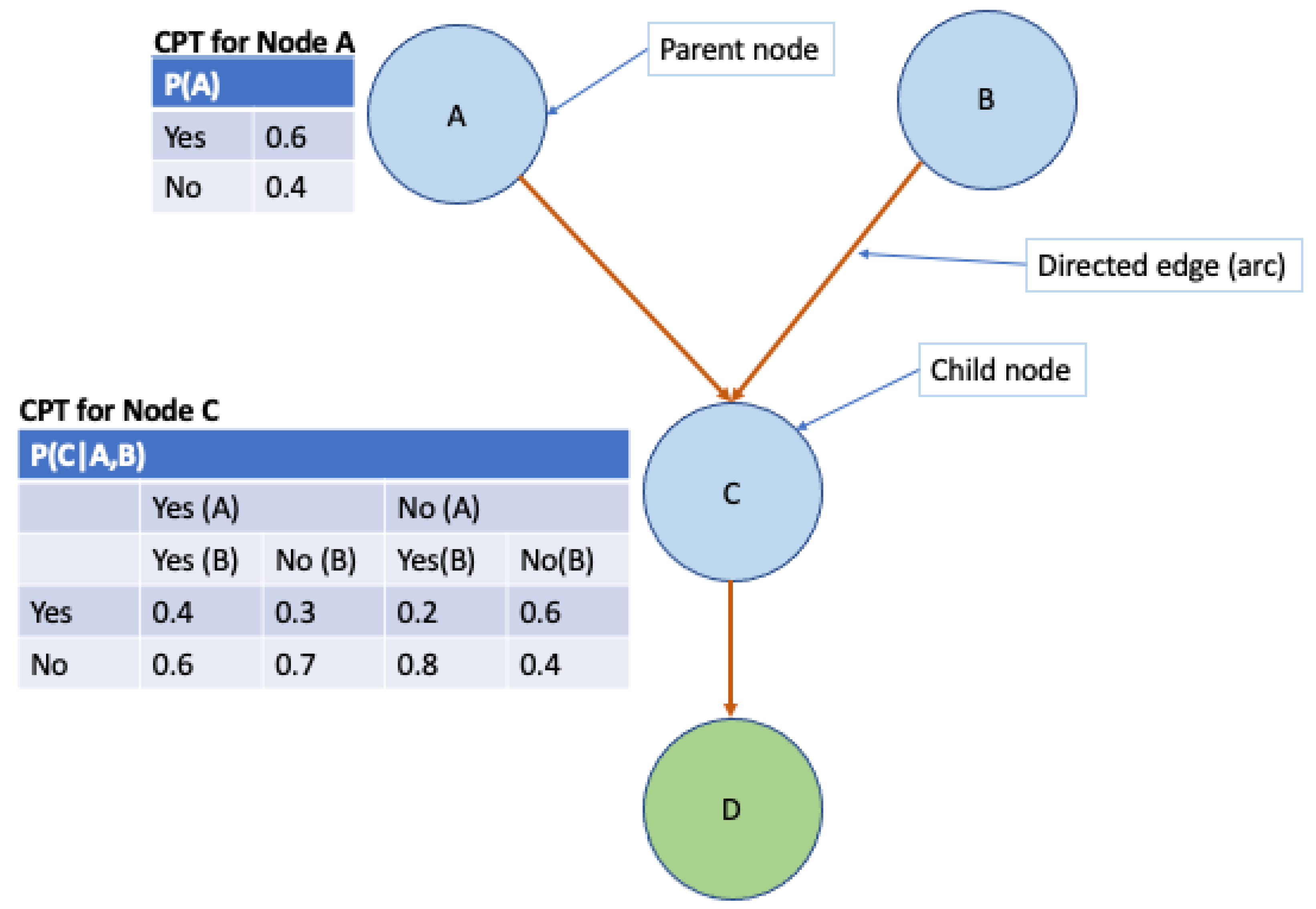
2.1. Bayesian Networks
2.2. Structured Expert Judgement
2.3. The SEJ Workshop
2.4. Data
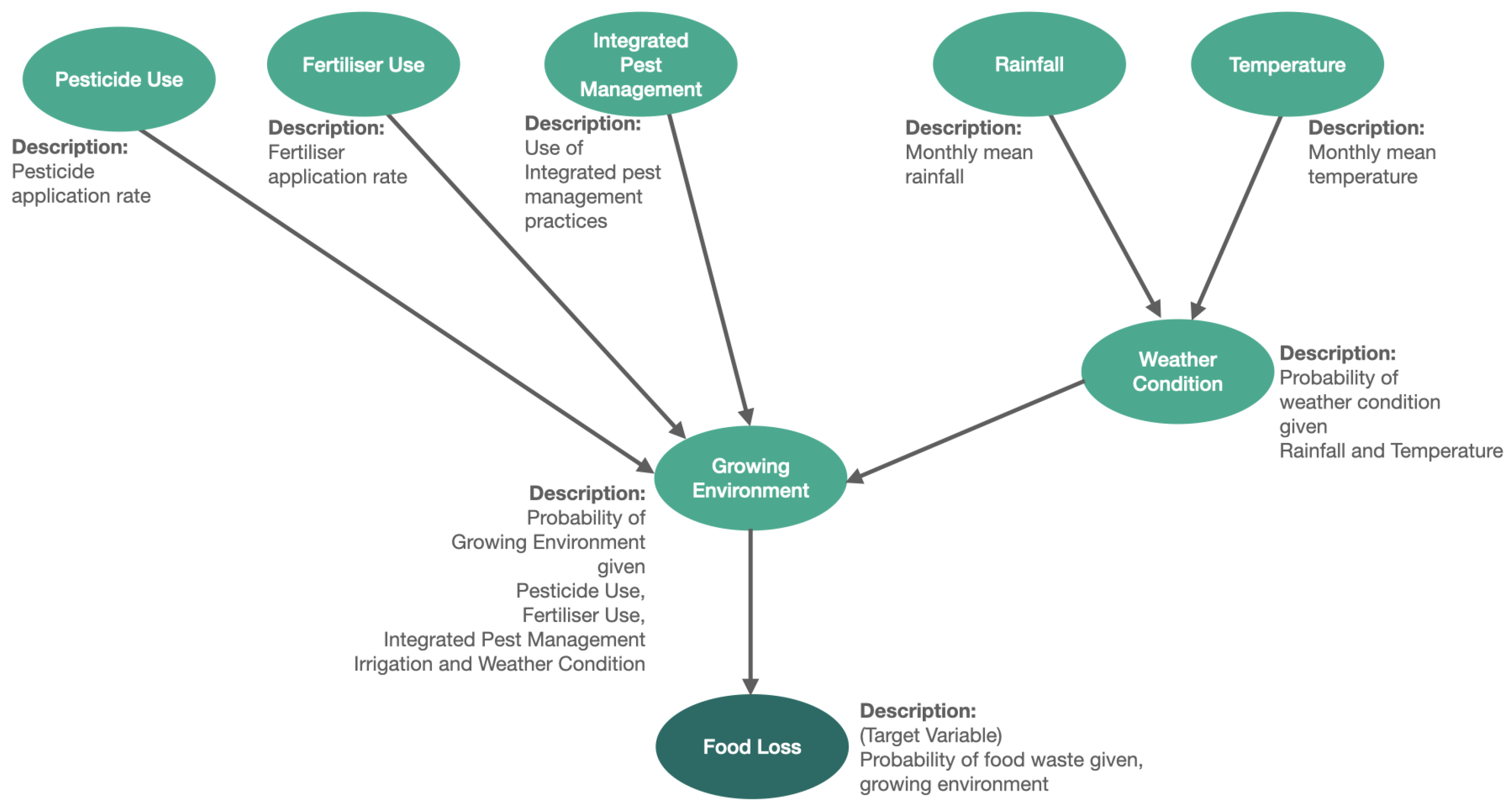
2.5. Model Development
3. Results
4. Conclusions
Author Contributions
Funding
Institutional Review Board Statement
Data Availability Statement
Acknowledgments
Conflicts of Interest
Appendix A


References
- Oerke, E.C. Crop losses to pests. J. Agric. Sci. 2006, 144, 31–43. [Google Scholar] [CrossRef]
- O’Connor, T.; Kleemann, R.; Attard, J. Vulnerable vegetables and efficient fishers: A study of primary production food losses and waste in Ireland. J. Environ. Manag. 2022, 307, 114498. [Google Scholar] [CrossRef] [PubMed]
- Olson, S. An analysis of the biopesticide market now and where it is going. Outlooks Pest Manag. 2015, 26, 203–206. [Google Scholar] [CrossRef]
- Rani, A.; Kammar, V.; Keerthi, M.; Rani, V.; Majumder, S.; Pandey, K.; Singh, J. Biopesticides: An alternative to synthetic insecticides. In Microbial Technology for Sustainable Environment; Springer: Singapore, 2021; pp. 439–466. [Google Scholar]
- Zadoks, J. Fifty years of crop protection, 1950–2000. Wagening. J. Life Sci. 2003, 50, 181–193. [Google Scholar] [CrossRef]
- Dara, S.K. The new integrated pest management paradigm for the modern age. J. Integr. Pest Manag. 2019, 10, 12. [Google Scholar] [CrossRef]
- Kogan, M. Integrated pest management: Historical perspectives and contemporary developments. Annu. Rev. Entomol. 1998, 43, 243–270. [Google Scholar] [CrossRef]
- Alix, A.; Capri, E. Modern agriculture in Europe and the role of pesticides. In Advances in Chemical Pollution, Environmental Management and Protection; Elsevier: Amsterdam, The Netherlands, 2018; Volume 2, pp. 1–22. [Google Scholar]
- Marchand, P.A.; Robin, D. Evolution of Directive (EC) No 128/2009 of the European Parliament and of the Council establishing a framework for Community action to achieve the sustainable use of pesticides. J. Regul. Sci. 2019, 7, 111. [Google Scholar] [CrossRef]
- Beausang, C.; Hall, C.; Toma, L. Food waste and losses in primary production: Qualitative insights from horticulture. Resour. Conserv. Recycl. 2017, 126, 177–185. [Google Scholar] [CrossRef]
- Lefèvre, A.; Perrin, B.; Lesur-Dumoulin, C.; Salembier, C.; Navarrete, M. Challenges of complying with both food value chain specifications and agroecology principles in vegetable crop protection. Agric. Syst. 2020, 185, 102953. [Google Scholar] [CrossRef]
- VI. Voluntary Initiative, IPM Hub, 2023. Available online: https://voluntaryinitiative.org.uk/schemes/integrated-pest-management/ (accessed on 17 November 2023).
- Rossi, V.; Sperandio, G.; Caffi, T.; Simonetto, A.; Gilioli, G. Critical success factors for the adoption of decision tools in IPM. Agronomy 2019, 9, 710. [Google Scholar] [CrossRef]
- Food and Agriculture Organization of the United Nations. Food Loss and Food Waste. 2021. Available online: https://www.fao.org/policy-support/policy-themes/food-loss-food-waste/en/ (accessed on 7 October 2020).
- Stenberg, J.A. A conceptual framework for integrated pest management. Trends Plant Sci. 2017, 22, 759–769. [Google Scholar] [CrossRef]
- Karlsson Green, K.; Stenberg, J.A.; Lankinen, Å. Making sense of Integrated Pest Management (IPM) in the light of evolution. Evol. Appl. 2020, 13, 1791–1805. [Google Scholar] [CrossRef]
- Fernandez-Cornejo, J.; Ferraioli, J. The environmental effects of adopting IPM techniques: The case of peach producers. J. Agric. Appl. Econ. 1999, 31, 551–564. [Google Scholar] [CrossRef]
- Walsh, L. Going green: Addressing challenges to sustainability in Irish horticulture. TResearch 2021, 16, 8–10. [Google Scholar]
- Lamichhane, J.R.; Arendse, W.; Dachbrodt-Saaydeh, S.; Kudsk, P.; Roman, J.C.; van Bijsterveldt-Gels, J.E.; Wick, M.; Messéan, A. Challenges and opportunities for integrated pest management in Europe: A telling example of minor uses. Crop Prot. 2015, 74, 42–47. [Google Scholar] [CrossRef]
- Barrière, V.; Lecompte, F.; Nicot, P.C.; Maisonneuve, B.; Tchamitchian, M.; Lescourret, F. Lettuce cropping with less pesticides. A review. Agron. Sustain. Dev. 2014, 34, 175–198. [Google Scholar] [CrossRef]
- Wang, L.; Ning, S.; Zheng, W.; Guo, J.; Li, Y.; Li, Y.; Chen, X.; Ben-Gal, A.; Wei, X. Performance analysis of two typical greenhouse lettuce production systems: Commercial hydroponic production and traditional soil cultivation. Front. Plant Sci. 2023, 14, 1165856. [Google Scholar] [CrossRef]
- Harwood, T.D.; Al Said, F.A.; Pearson, S.; Houghton, S.J.; Hadley, P. Modelling uncertainty in field grown iceberg lettuce production for decision support. Comput. Electron. Agric. 2010, 71, 1. [Google Scholar] [CrossRef]
- Gallardo, M.; Elia, A.; Thompson, R.B. Decision support systems and models for aiding irrigation and nutrient management of vegetable crops. Agric. Water Manag. 2020, 240, 106209. [Google Scholar] [CrossRef]
- Drury, B.; Valverde-Rebaza, J.; Moura, M.-F.; de Andrade Lopes, A. A survey of the applications of Bayesian networks in agriculture. Eng. Appl. Artif. Intell. 2017, 65, 29–42. [Google Scholar] [CrossRef]
- Barons, M.J.; Wright, S.K.; Smith, J.Q. Eliciting probabilistic judgements for integrating decision support systems. In Elicitation; Springer: Cham, Switzerland, 2018; pp. 445–478. [Google Scholar]
- Nyberg, E.P.; Nicholson, A.E.; Korb, K.B.; Wybrow, M.; Zukerman, I.; Mascaro, S.; Thakur, S.; Alvandi, A.O.; Riley, J.; Pearson, R.; et al. BARD: A Structured Technique for Group Elicitation of Bayesian networks to Support Analytic Reasoning. Risk Anal. 2021, 42, 6. [Google Scholar] [CrossRef]
- Ticehurst, J.L.; Letcher, R.A.; Rissik, D. Integration modelling and decision support: A case study of the coastal lake assessment and management (CLAM) tool. Math. Comput. Simul. 2008, 78, 435–499. [Google Scholar] [CrossRef]
- Keeney, R.L.; Raiffa, H. Decisions with Multiple Objectives Preferences and Value Trade-Offs; Cambridge University Press: Cambridge, UK, 1993. [Google Scholar]
- Korb, K.; Nicholson, A. Bayesian Artificial Intelligence, 2nd ed.; Chapman and Hall: London, UK, 2010. [Google Scholar]
- Steeneveld, W.; van der Gaag, M.A.; Barkema, H.W.; Hogeveen, H. Bayesian networks for mastitis management on dairy farms. In Proceedings of the Society for Veterinary Epidemiology and Preventive Medicine, London, UK, 1–3 April 2009; pp. 126–135. [Google Scholar]
- Holt, J.; Mushobozi, W.; Day, R.K.; Knight, J.D.; Kimani, M.; Njuki, J.; Musebe, R. A simple Bayesian network to interpret the accuracy of armyworm outbreak forecasts. Ann. Appl. Biol. 2006, 148, 141–146. [Google Scholar] [CrossRef]
- Aguilera, P.A.; Fernández, A.; Ropero, R.F.; Molina, L. Groundwater quality assessment using data clustering based on hybrid Bayesian networks. Stoch. Environ. Res. Risk Assess. 2013, 27, 2. [Google Scholar] [CrossRef]
- Sun, L.; Zhu, Z.S. A Bayesian network model for aeration management of stored grain. Appl. Mech. Mater. 2013, 380, 4751–4756. [Google Scholar] [CrossRef]
- van der Gaag, L.C.; Bolt, J.; Loeffen, W.; Elbers, A. Modelling patterns of evidence in Bayesian networks: A case-study in classical swine fever. In Computational Intelligence for Knowledge-Based Systems Design; Lecture Notes in Computer Science; Springer: Berlin/Heidelberg, Germany, 2010; pp. 675–684. [Google Scholar]
- Smith, J.Q.; Barons, M.; Leonelli, M. Coherent inference for Integrating Decision Support Systems. arXiv 2016, arXiv:1507.07394. [Google Scholar]
- Smith, J.Q.; Barons, M.J.; Leonelli, M. Decision focused inference on networked probabilistic systems: With applications to food security. In Proceedings of the JSM Proceedings 2015, Seattle, WA, USA, 8–13 August 2015; pp. 3220–3233. [Google Scholar]
- Pearl, J. Bayesian networks A Model of Self-Activated Memory for Evidential Reasoning. In Proceedings of the Seventh Annual Conference of the Cognitive Science Society, Irvine, CA, USA, 15–17 August 1985. [Google Scholar]
- Koller, D.; Friedman, N. Probabilistic Graphical Models: Principles and Techniques; MIT Press: Cambridge, MA, USA, 2009. [Google Scholar]
- Murphy, K.P. Machine Learning: A Probabilistic Perspective; MIT Press: Cambridge, MA, USA, 2012. [Google Scholar]
- Barons, M.J.; Mascaro, S.; Hanea, A.M. Balancing the Elicitation Burden and the Richness of Expert Input When Quantifying Discrete Bayesian networks. Risk Anal. 2022, 42, 1196–1234. [Google Scholar] [CrossRef]
- Kahneman, D.; Tversky, A. Choices, values, and frames. Am. Psychol. 1984, 39, 341–350. [Google Scholar] [CrossRef]
- Slovic, P. Trust, emotion, sex, politics, and science: Surveying the risk-assessment battle field. Risk Anal. 1999, 19, 689–701. [Google Scholar] [CrossRef]
- O’Hagan, A.; Buck, C.; Daneshkhah, A.; Eiser, J.; Garthwaite, P.; Jenkinson, D.; Oakley, J.; Rakow, T. Uncertain Judgements: Eliciting Experts’ Probabilities; Wiley: London, UK, 2006. [Google Scholar]
- Cooke, R.; Goossens, L. TU Delft expert judgment data base. Reliab. Eng. Syst. Saf. 2008, 93, 657–674. [Google Scholar] [CrossRef]
- Aspinall, W. A route to more tractable expert advice. Nature 2010, 463, 294–295. [Google Scholar] [CrossRef] [PubMed]
- Burgman, M.A. Trusting Judgements: How to Get the Best out of Experts; Cambridge University Press: Cambridge, UK, 2015. [Google Scholar] [CrossRef]
- Bolger, F.; Hanea, A.; O’Hagan, A.; Mosbach-Schulz, O.; Oakley, J.; Rowe, G.; Wenholt, M. Guidance on Expert Knowledge Elicitation in Food and Feed Safety Risk Assessment. EFSA J. 2014, 12, 3734. [Google Scholar]
- Cooke, R.; Wilson, A.; Tuomisto, J.; Morales Napoles, O.; Tainio, M.; Evans, J. A probabilistic characterization of the relationship between fine particulate matter and mortality: Elicitation of European experts. Environ. Sci. Technol. 2007, 41, 6598–6605. [Google Scholar] [CrossRef]
- Kleve, S.; Barons, M.J. A Structured Expert Judgement elicitation approach: How can it inform sound intervention decision making to support household food security? Public Health Nutr. 2021, 24, 2050–2061. [Google Scholar] [CrossRef] [PubMed]
- Krayer von Krauss, M.P.; Casman, E.A.; Small, M.J. Elicitation of Expert Judgments of Uncertainty in the Risk Assessment of Herbicide-Tolerant Oilseed Crops. Risk Anal. 2004, 24, 1515–1527. [Google Scholar] [CrossRef] [PubMed]
- Hanea, A.; McBride, M.; Burgman, M.; Wintle, B. Classical meets modern in the IDEA protocol for structured expert judgement. J. Risk Res. 2018, 21, 417–433. [Google Scholar] [CrossRef]
- Cooke, R.; Thijs, M.M.W. Calibration and information in expert resolution; a classical approach. Automatica 1988, 24, 87–93. [Google Scholar] [CrossRef]
- French, S. From soft to hard elicitation. J. Oper. Res. Soc. 2022, 73, 1181–1197. [Google Scholar] [CrossRef]
- Pigeon, M.; Jacques, M.; Goulet, V. R Expert: Modeling without Data Using Expert Opinion. 2008. Available online: https://cran.r-project.org/package=expert (accessed on 11 March 2021).
- Barzman, M.; Bàrberi, P.; Birch, A.N.E.; Boonekamp, P.; Dachbrodt-Saaydeh, S.; Graf, B.; Hommel, B.; Jensen, J.E.; Kiss, J.; Kudsk, P.; et al. Eight principles of integrated pest management. Agron. Sustain. Dev. 2015, 35, 1199–1215. [Google Scholar] [CrossRef]
- Lane, D.E.; Walker, T.J.; Grantham, D.G. IPM adoption and impacts in the United States. J. Integr. Pest Manag. 2023, 14, 1. [Google Scholar] [CrossRef]


| Data | Source |
|---|---|
| Fungicide Application Rate (kg/ha) | Food and Environment Research Agency (FERA) |
| Insecticide Application Rate (kg/ha) | Food and Environment Research Agency (FERA) |
| Herbicide Application Rate (kg/ha) | Food and Environment Research Agency (FERA) |
| Molluscicide Application Rate (kg/ha) | Food and Environment Research Agency (FERA) |
| Reduction in Pesticide Use (%) | Structured Expert Judgement |
| Reduction in Fertiliser Use (%) | Structured Expert Judgement |
| Integrated Pest Management (IPM) | Structured Expert Judgement |
| Food Loss (%) | Structured Expert Judgement |
| Pesticide | Application Rate Intervals | Categories |
|---|---|---|
| Fungicide | 0.019–0.349 kg/ha | Q1 |
| 0.350–0.645 kg/ha | Q2 | |
| 0.646–5.000 kg/ha | Q3 | |
| Herbicide | 0.151–0.550 kg/ha | Q1 |
| 0.551–0.709 kg/ha | Q2 | |
| 0.710–1.800 kg/ha | Q3 | |
| Insecticide | 0.0042–0.0538 kg/ha | Q1 |
| 0.0539–0.0793 kg/ha | Q2 | |
| 0.0794–0.2000 kg/ha | Q3 | |
| Molluscicide | 0.135–0.146 kg/ha | Q1 |
| 0.147–0.171 kg/ha | Q2 | |
| 0.172–0.232 kg/ha | Q3 |
| Question | Percentile | ||
|---|---|---|---|
| 5th | 50th | 95th | |
| What is the percentage change in the expected crop yield if... | |||
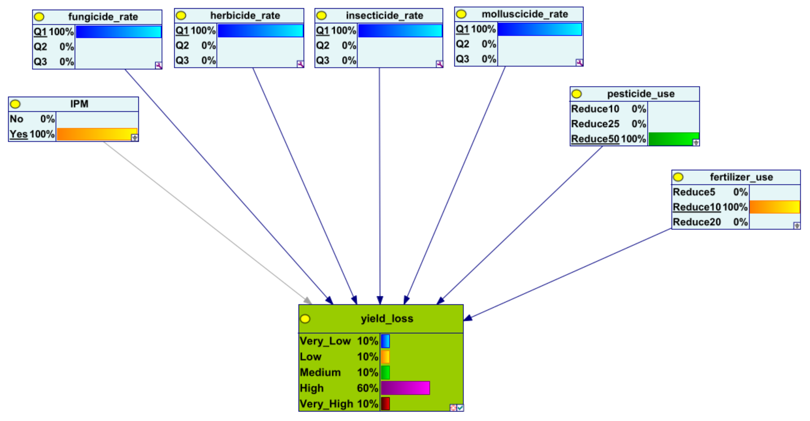
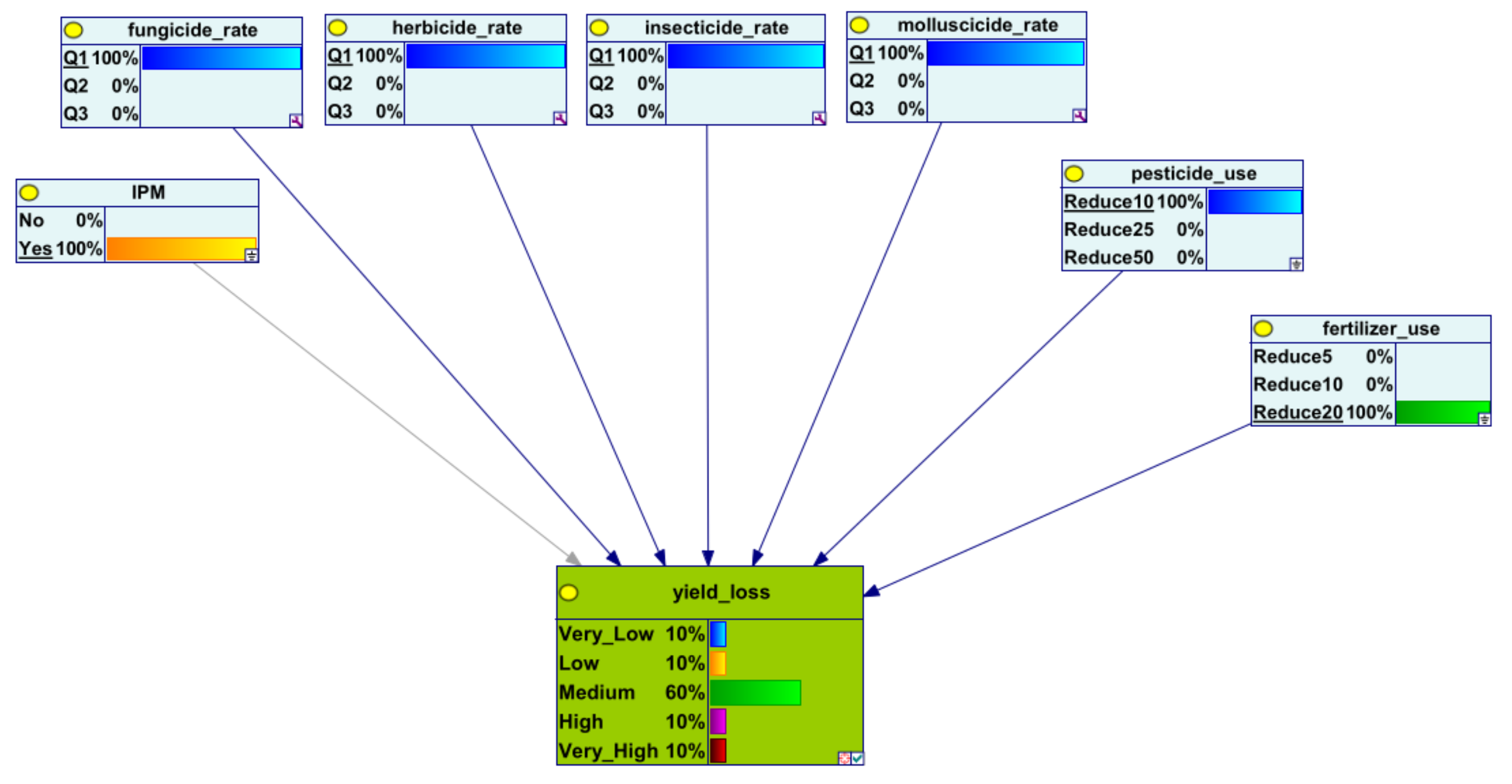
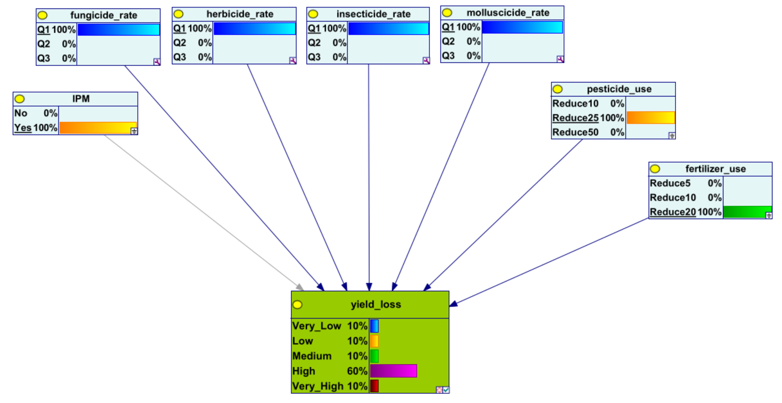
| IPM is unchanged, pesticide use is reduced by 10% and fertiliser is reduced by 5%? | −7.917 | −3.500 | −1.417 |
| IPM is unchanged, pesticide use is reduced by 10% and fertiliser is reduced by 10%? | −10.000 | −6.667 | −4.333 |
| IPM is unchanged, pesticide use is reduced by 10% and fertiliser is reduced by 20%? | −18.833 | −13.000 | −8.500 |
| IPM is unchanged, pesticide use is reduced by 25% and fertiliser is reduced by 5%? | −16.667 | −8.667 | −6.000 |
| IPM is unchanged, pesticide use is reduced by 25% and fertiliser is reduced by 10%? | −18.083 | −12.833 | −8.250 |
| IPM is unchanged, pesticide use is reduced by 25% and fertiliser is reduced by 20%? | −24.583 | −18.500 | −11.083 |
| IPM is unchanged, pesticide use is reduced by 50% and fertiliser is reduced by 5%? | −26.250 | −14.833 | −10.750 |
| IPM is unchanged, pesticide use is reduced by 50% and fertiliser is reduced by 10%? | −28.167 | −19.333 | −12.000 |
| IPM is unchanged, pesticide use is reduced by 50% and fertiliser is reduced by 20%? | −37.500 | −25.333 | −18.833 |
| IPM is increased, pesticide use is reduced by 10% and fertiliser is reduced by 5%? | −4.083 | 1.333 | 4.083 |
| IPM is increased, pesticide use is reduced by 10% and fertiliser is reduced by 10%? | −6.833 | −3.167 | −0.833 |
| IPM is increased, pesticide use is reduced by 10% and fertiliser is reduced by 20%? | −14.000 | −8.833 | −4.667 |
| IPM is increased, pesticide use is reduced by 25% and fertiliser is reduced by 5%? | −12.083 | −5.750 | −1.750 |
| IPM is increased, pesticide use is reduced by 25% and fertiliser is reduced by 10%? | −14.833 | −9.917 | −4.667 |
| IPM is increased, pesticide use is reduced by 25% and fertiliser is reduced by 20%? | −20.000 | −13.917 | −9.167 |
| IPM is increased, pesticide use is reduced by 50% and fertiliser is reduced by 5%? | −23.750 | −13.917 | −9.167 |
| IPM is increased, pesticide use is reduced by 50% and fertiliser is reduced by 10%? | −24.167 | −17.167 | −11.167 |
| IPM is increased pesticide use is reduced by 50% and fertiliser is reduced by 20%? | −30.667 | −22.833 | −16.667 |
| % Reduction | Probability of Food Loss (%) | |||||||
|---|---|---|---|---|---|---|---|---|
| Q | IPM | Fertiliser | Pesticide | Very Low | Low | Medium | High | Very High |
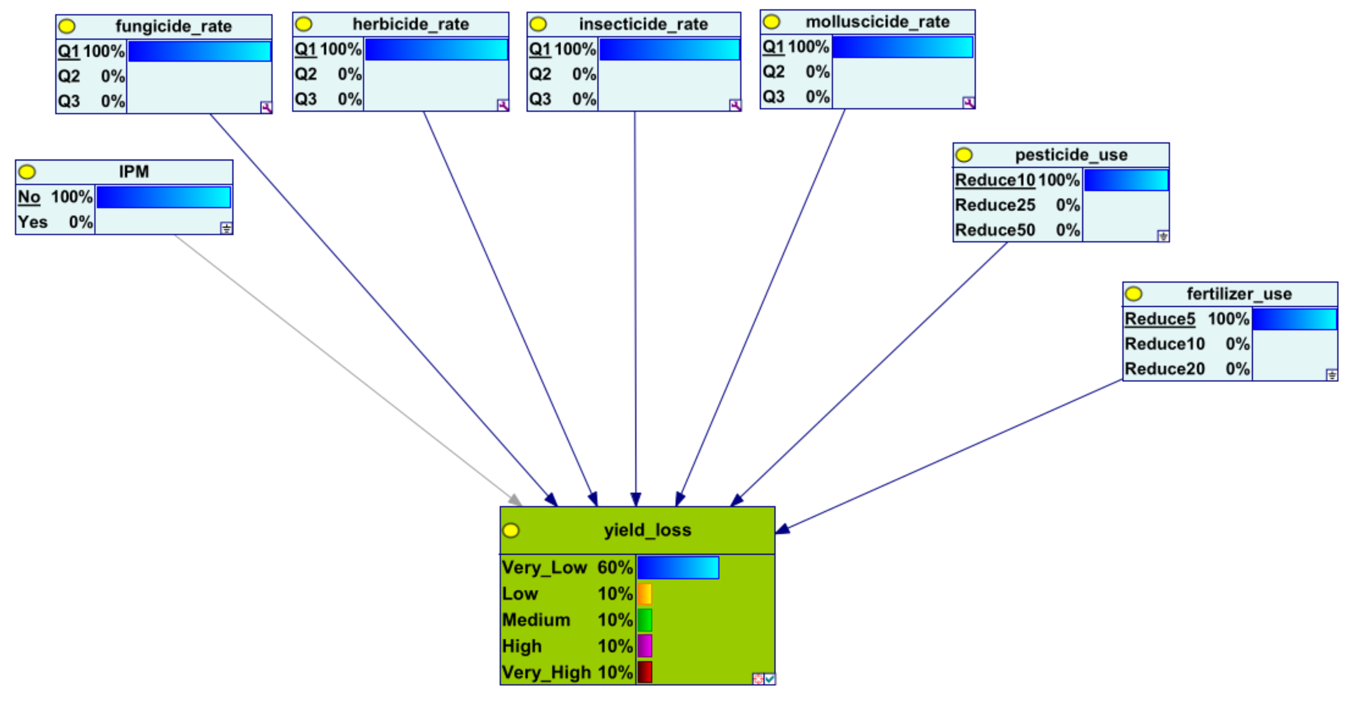
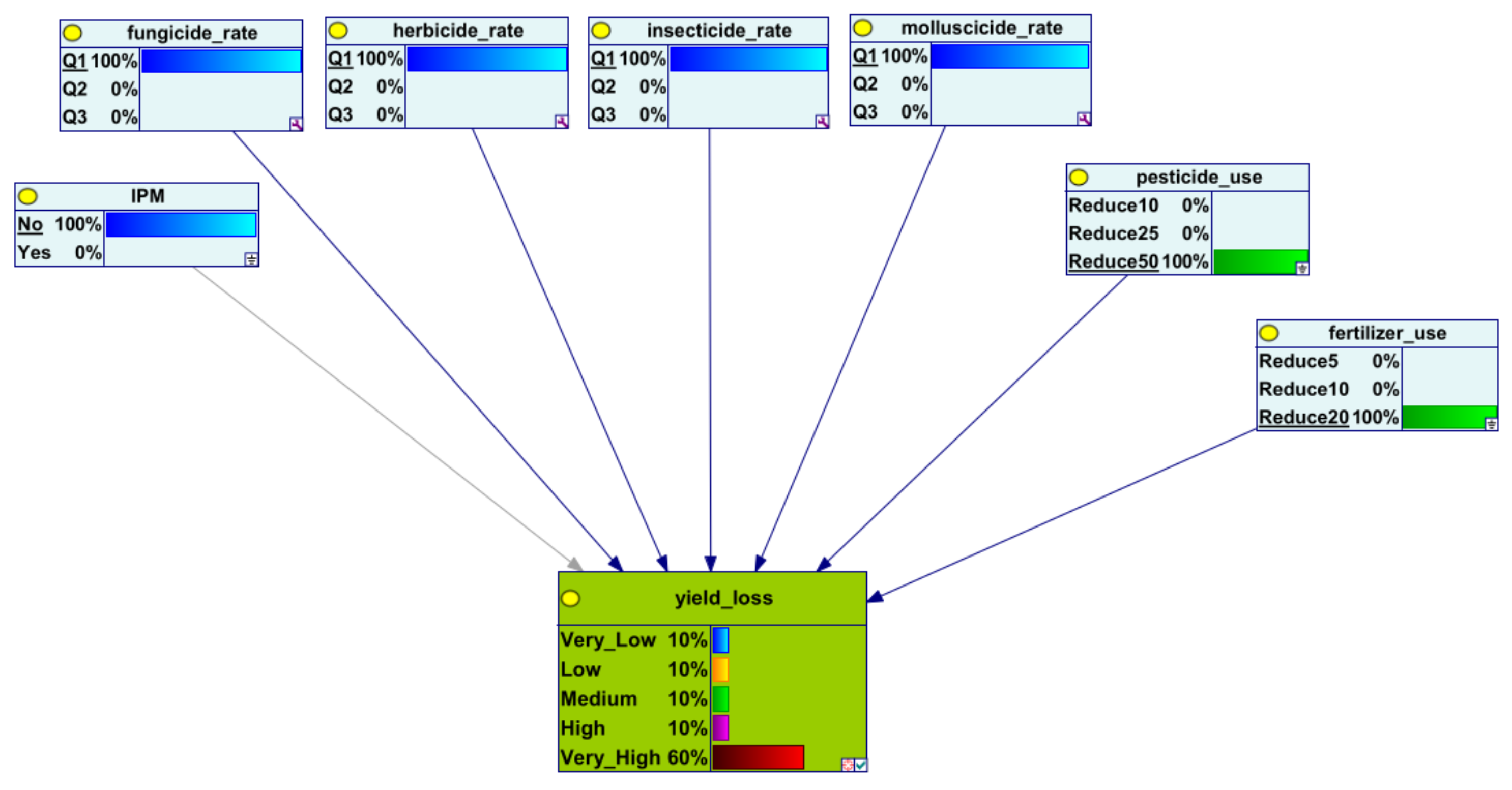
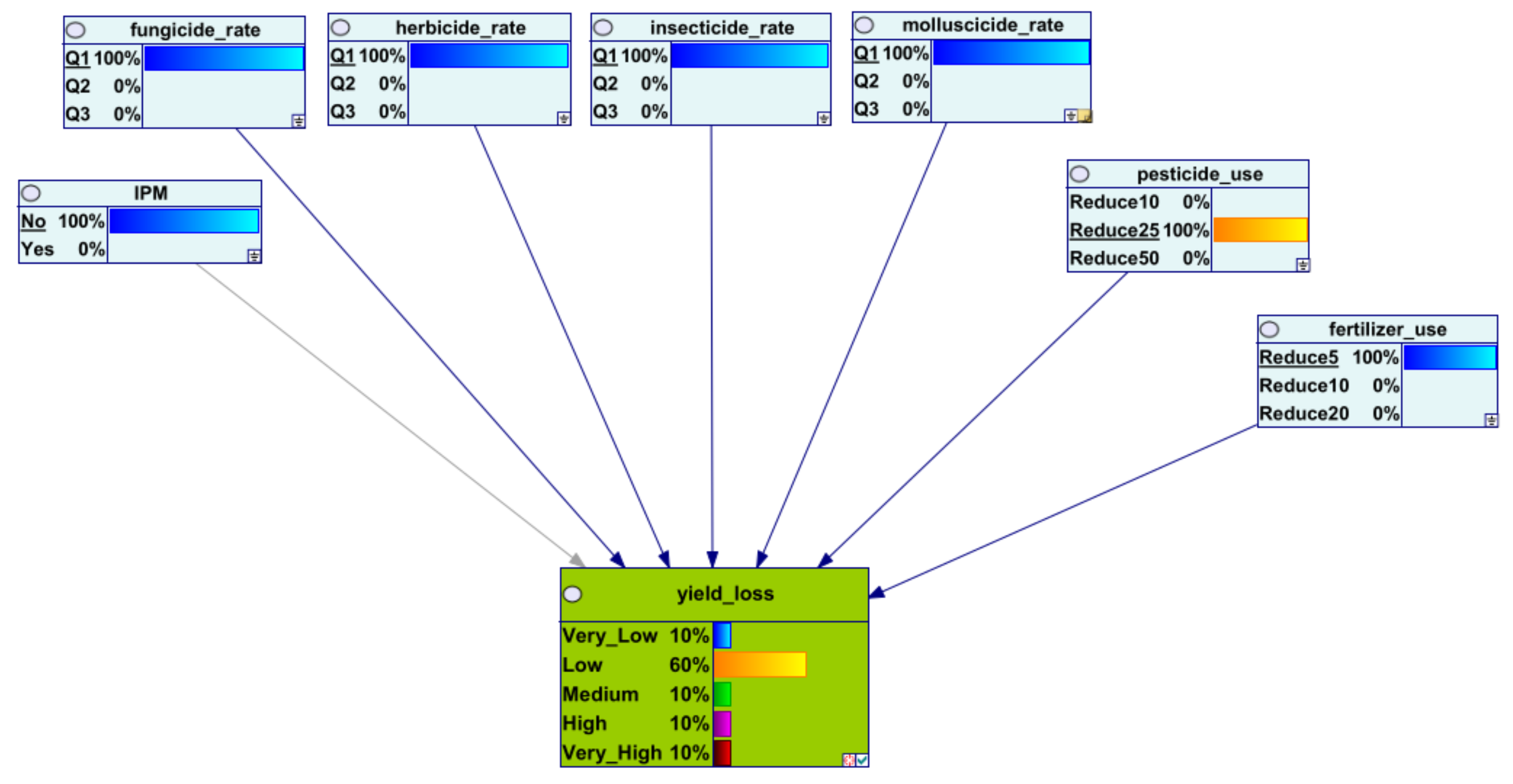
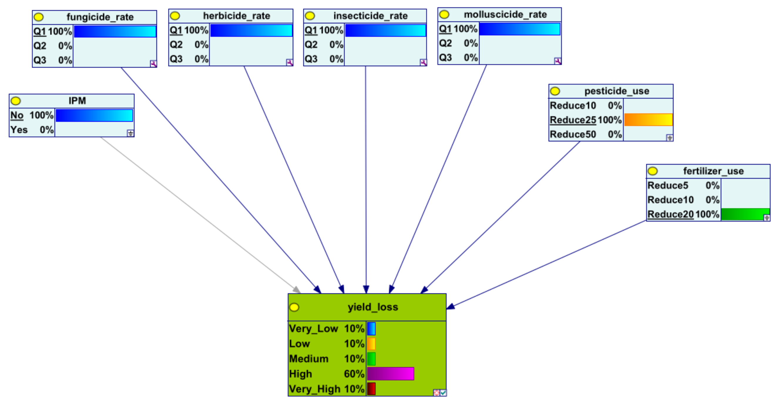
| 1 | No | 5 | 10 | 60 | 10 | 10 | 10 | 10 |
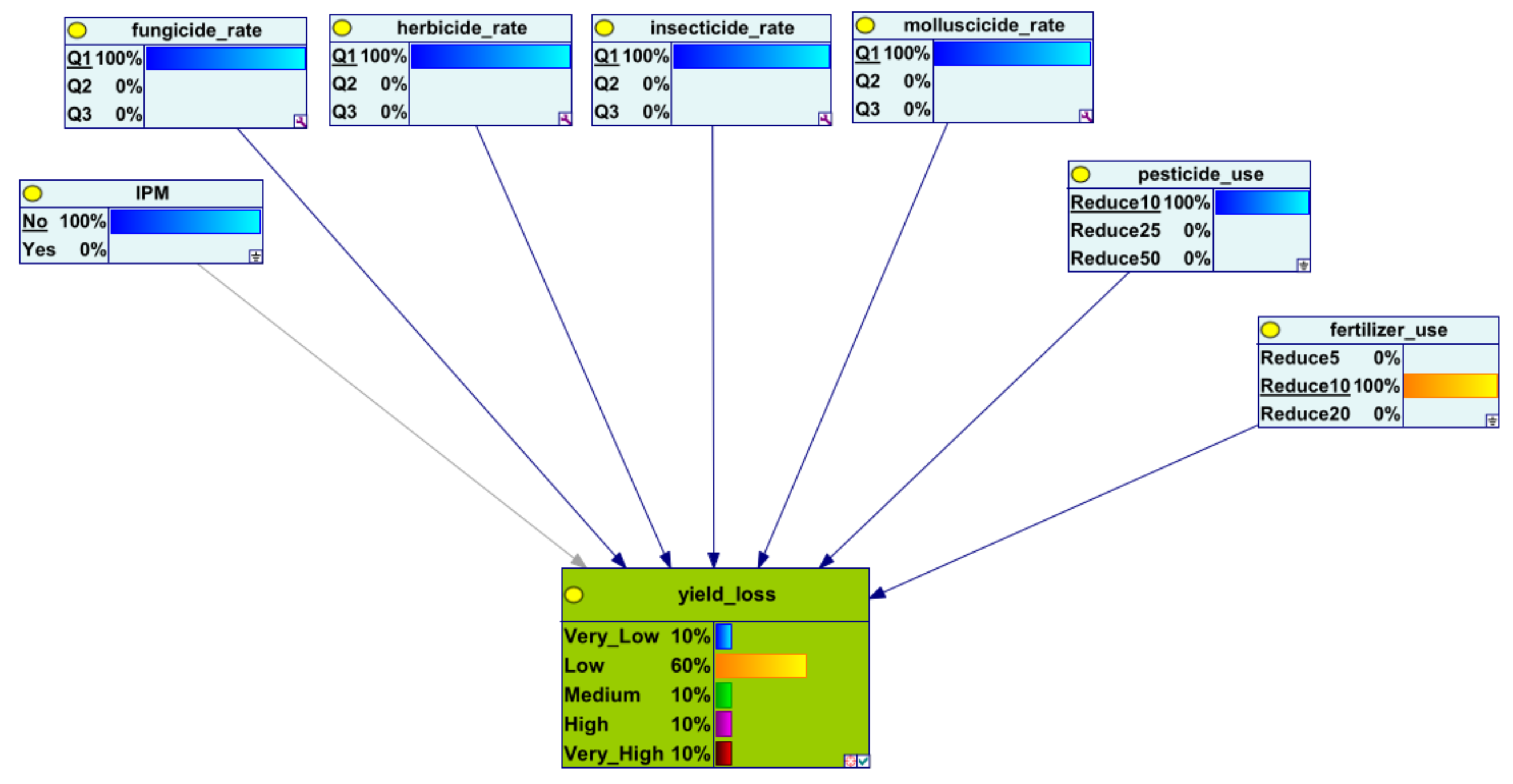
| 1 | No | 10 | 10 | 10 | 60 | 10 | 10 | 10 |
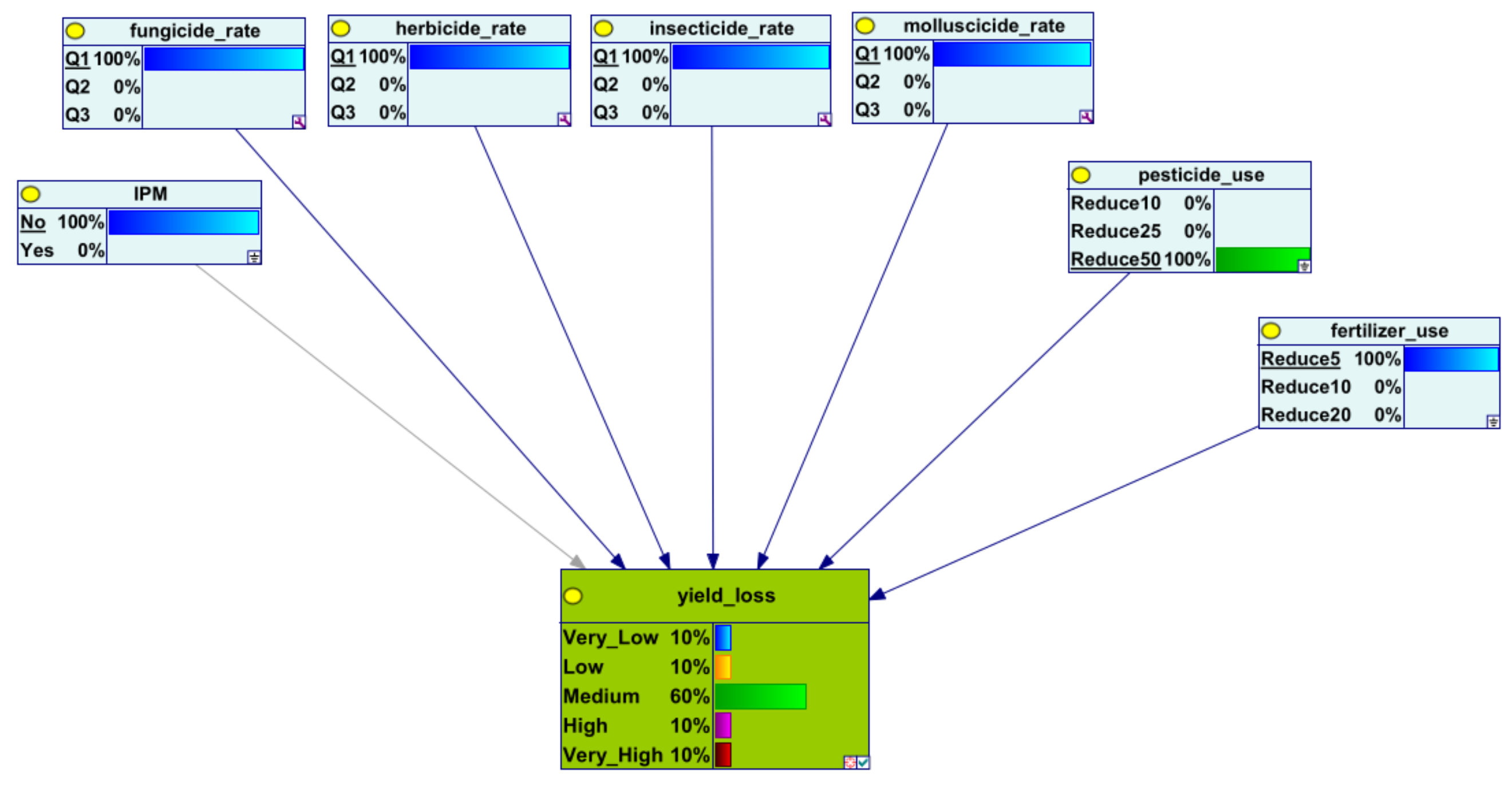
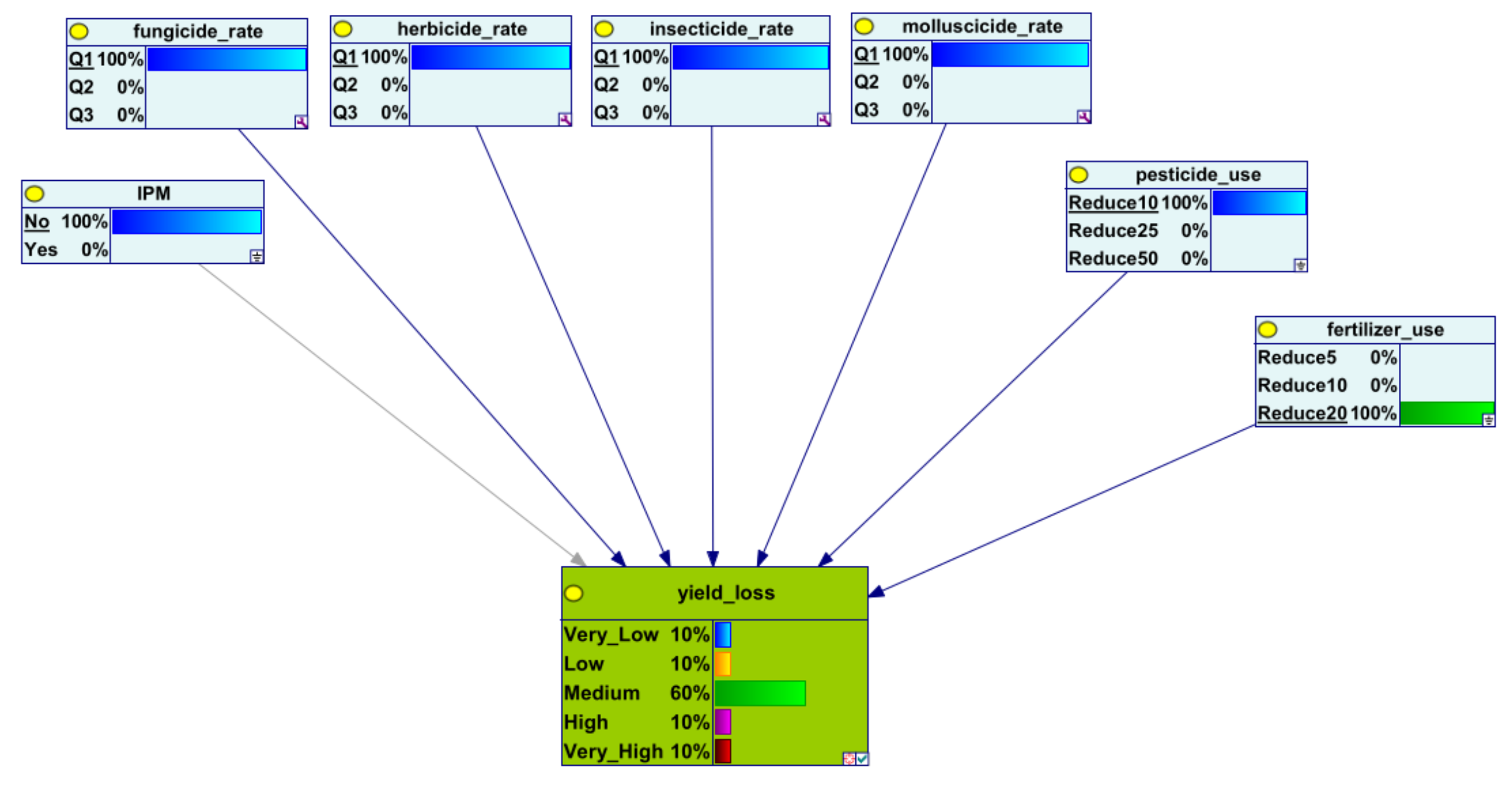
| 1 | No | 20 | 10 | 10 | 10 | 60 | 10 | 10 |
| 1 | No | 5 | 25 | 10 | 60 | 10 | 10 | 10 |
| 1 | No | 10 | 25 | 10 | 10 | 60 | 10 | 10 |
| 1 | No | 20 | 25 | 10 | 10 | 10 | 60 | 10 |
| 1 | No | 5 | 50 | 10 | 10 | 60 | 10 | 10 |
| 1 | No | 10 | 50 | 10 | 10 | 10 | 60 | 10 |
| 1 | No | 20 | 50 | 10 | 10 | 10 | 10 | 60 |
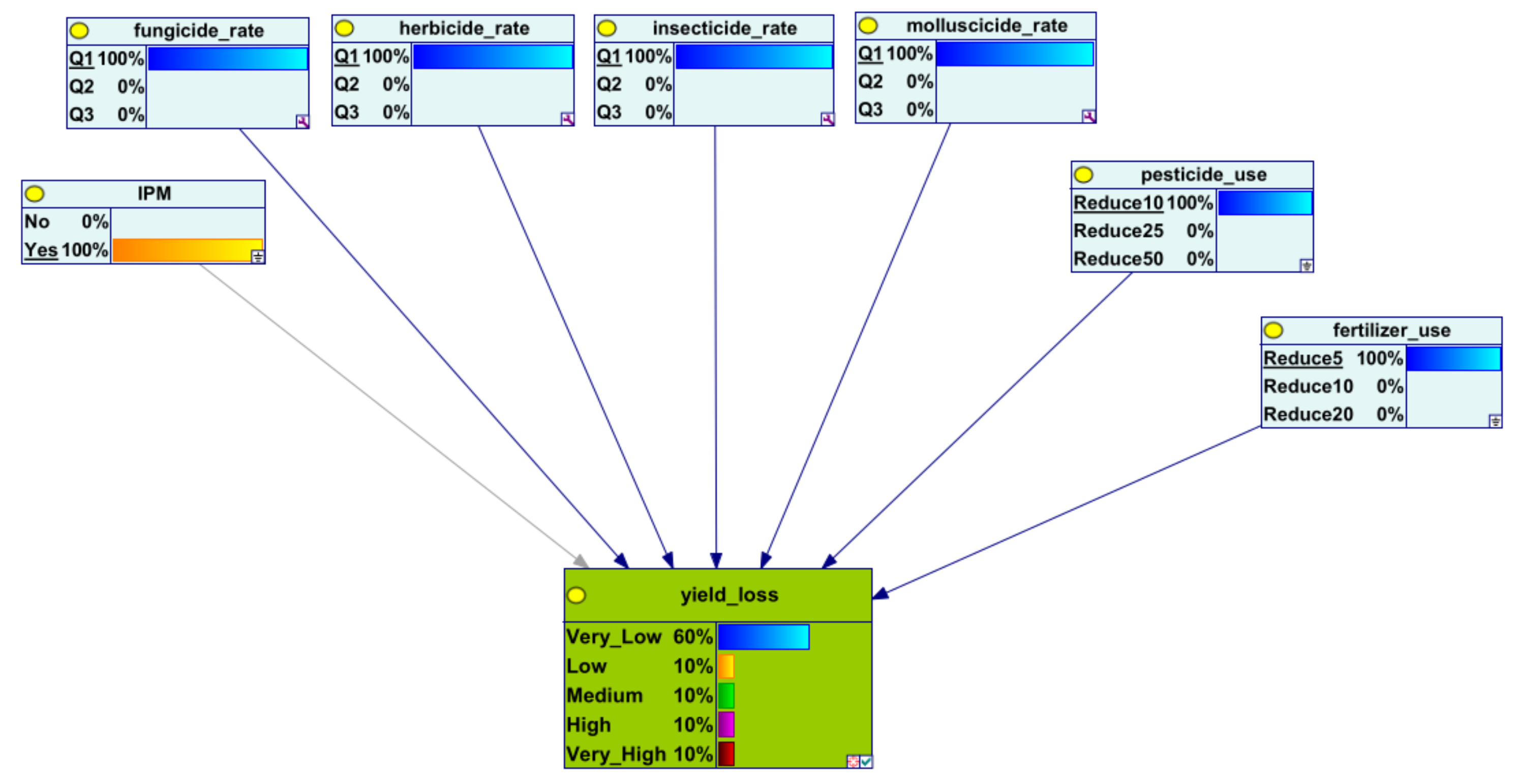
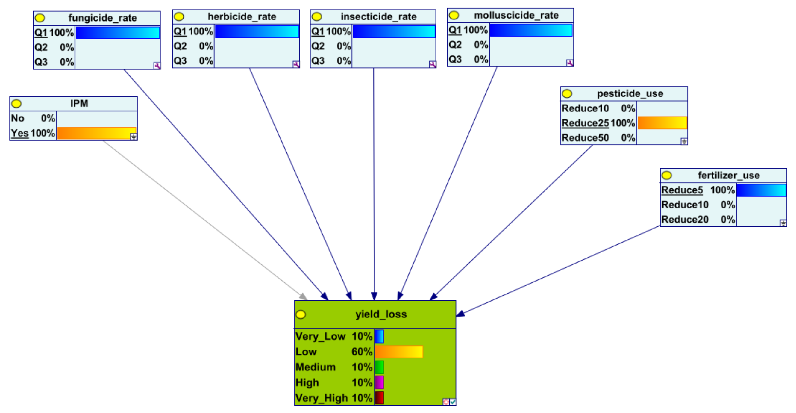
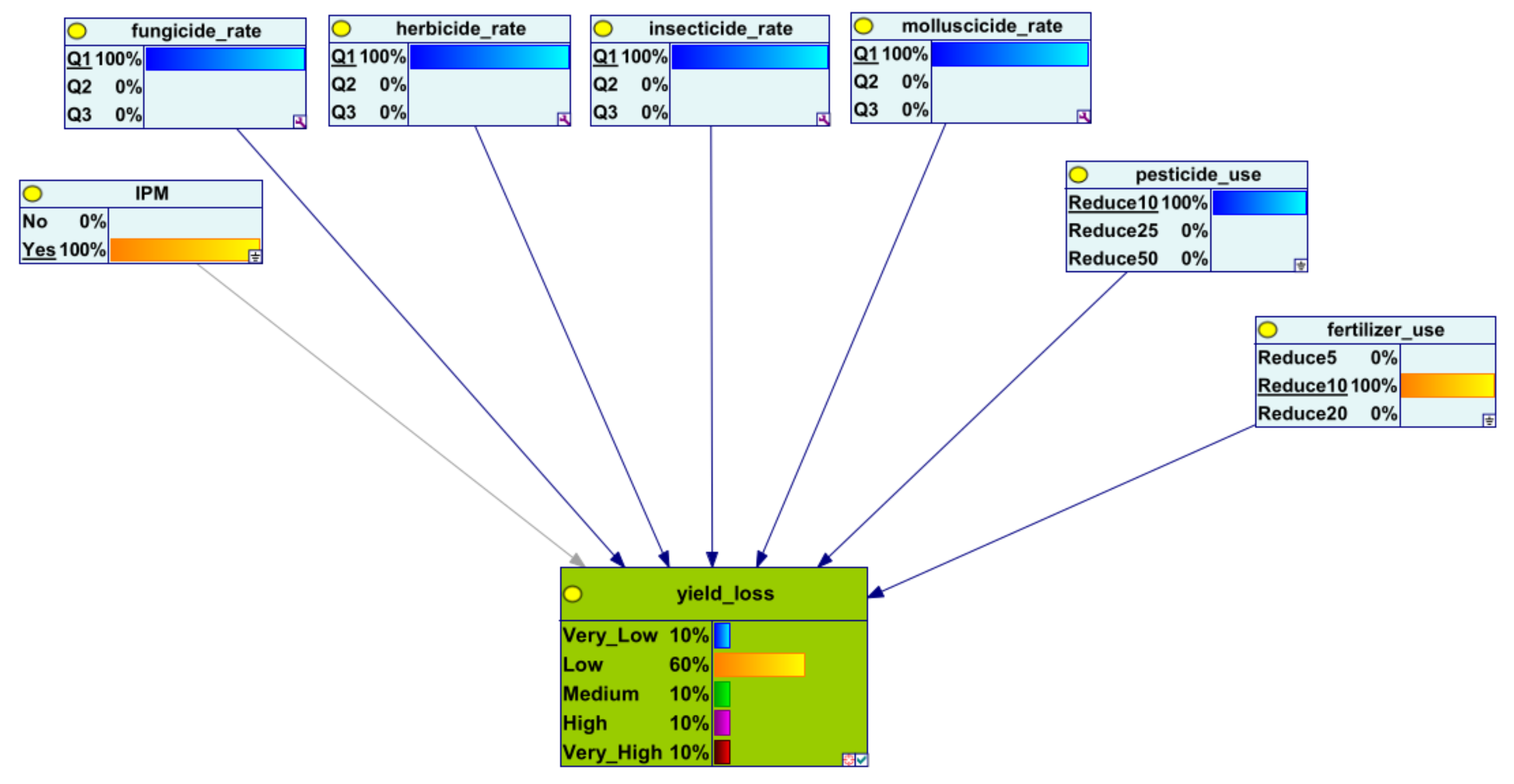
| 1 | Yes | 5 | 10 | 60 | 10 | 10 | 10 | 10 |
| 1 | Yes | 10 | 10 | 10 | 60 | 10 | 10 | 10 |
| 1 | Yes | 20 | 10 | 10 | 10 | 60 | 10 | 10 |
| 1 | Yes | 5 | 25 | 10 | 60 | 10 | 10 | 10 |
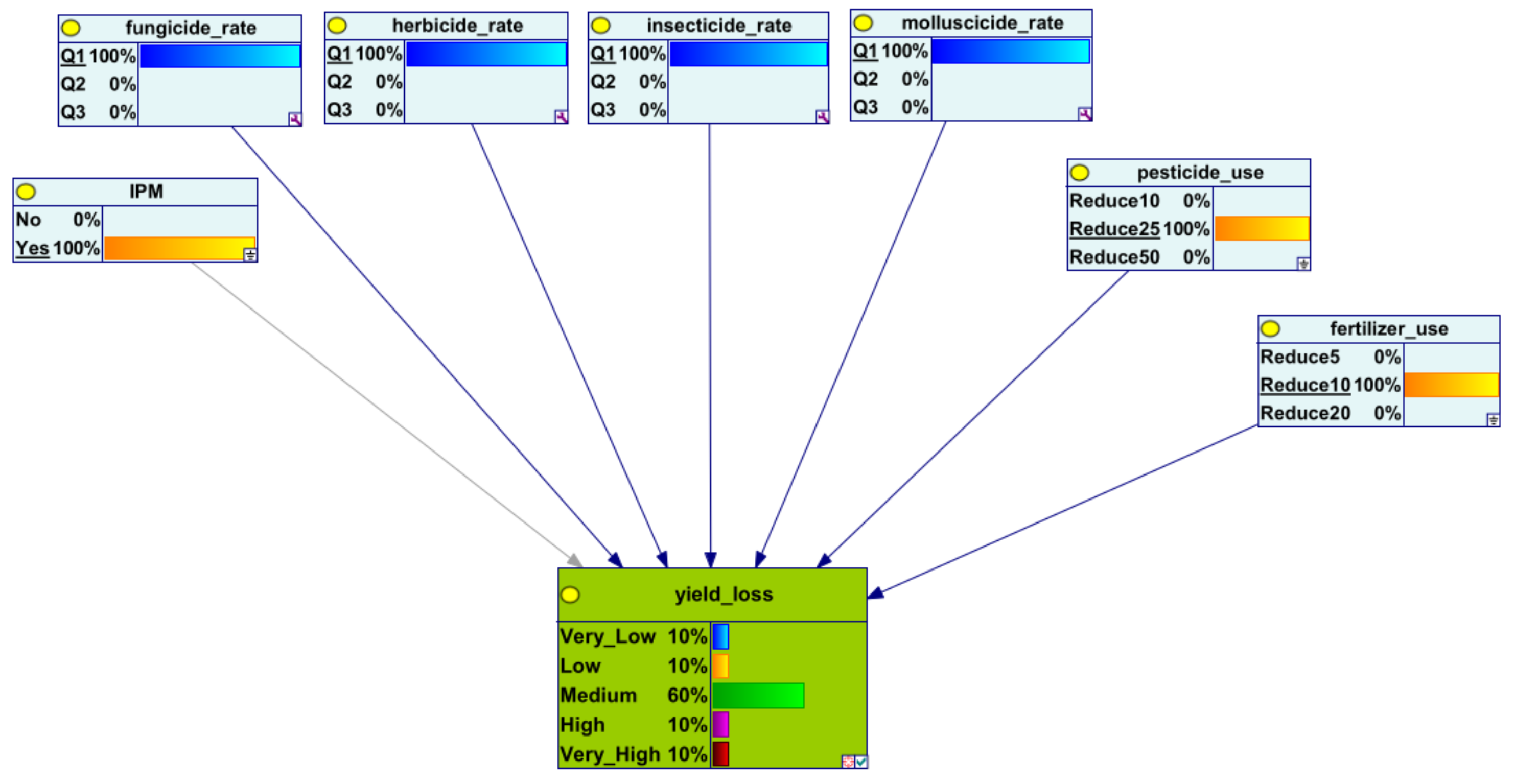
| 1 | Yes | 10 | 25 | 10 | 10 | 60 | 10 | 10 |
| 1 | Yes | 20 | 25 | 10 | 10 | 10 | 60 | 10 |
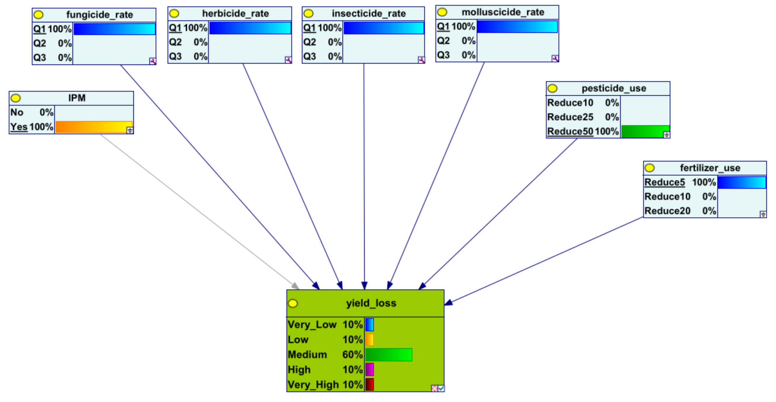
| 1 | Yes | 5 | 50 | 10 | 10 | 60 | 10 | 10 |
| 1 | Yes | 10 | 50 | 10 | 10 | 10 | 60 | 10 |
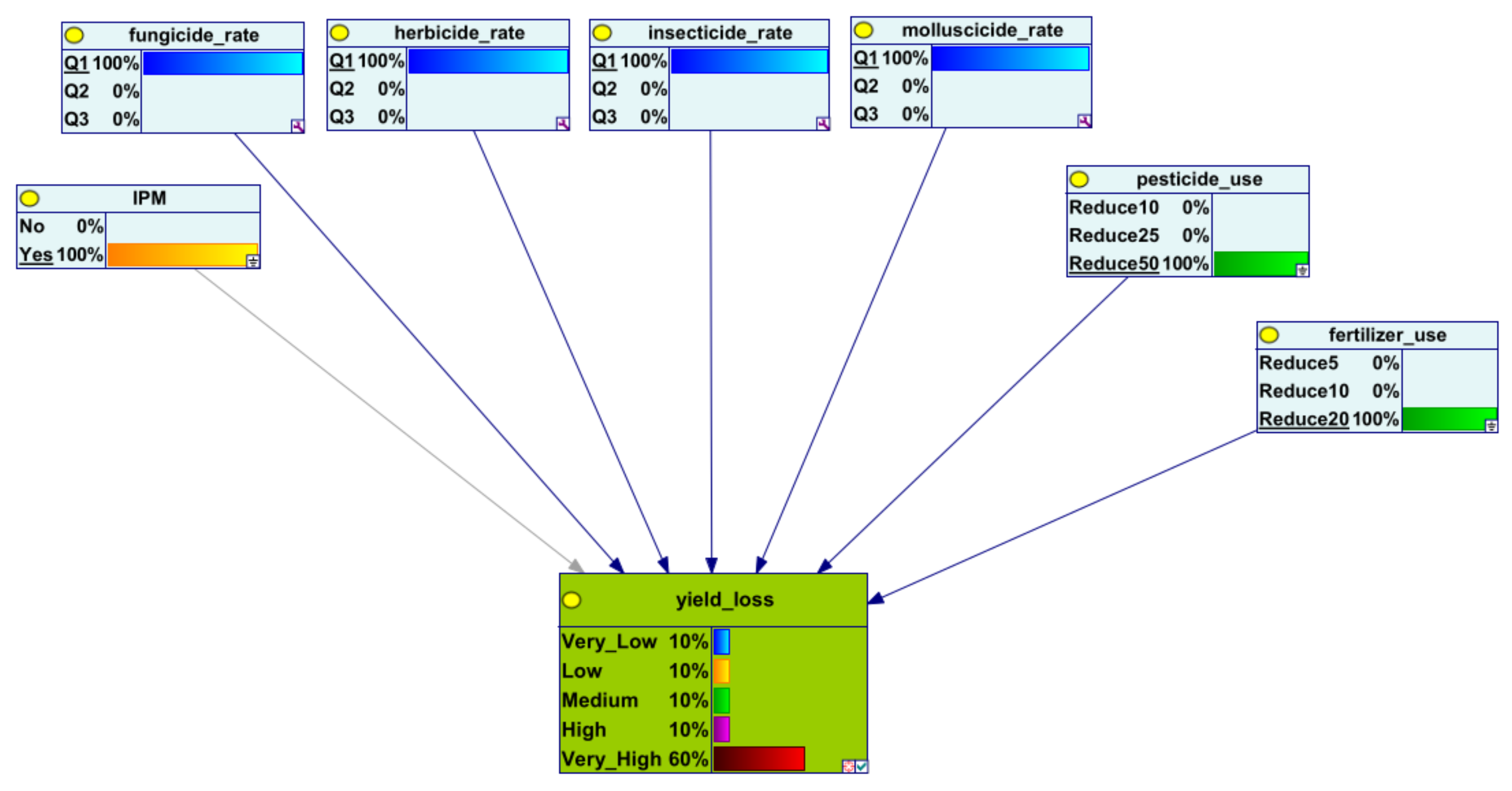
| 1 | Yes | 20 | 50 | 10 | 10 | 10 | 10 | 60 |
| % Reduction | Probability of Food Loss (%) | |||||||
|---|---|---|---|---|---|---|---|---|
| Q | IPM | Fertiliser | Pesticide | Very Low | Low | Medium | High | Very High |
| 2 | No | 10 | 5 | 60 | 10 | 10 | 10 | 10 |
| 2 | No | 10 | 10 | 10 | 60 | 10 | 10 | 10 |
| 2 | No | 10 | 20 | 10 | 10 | 60 | 10 | 10 |
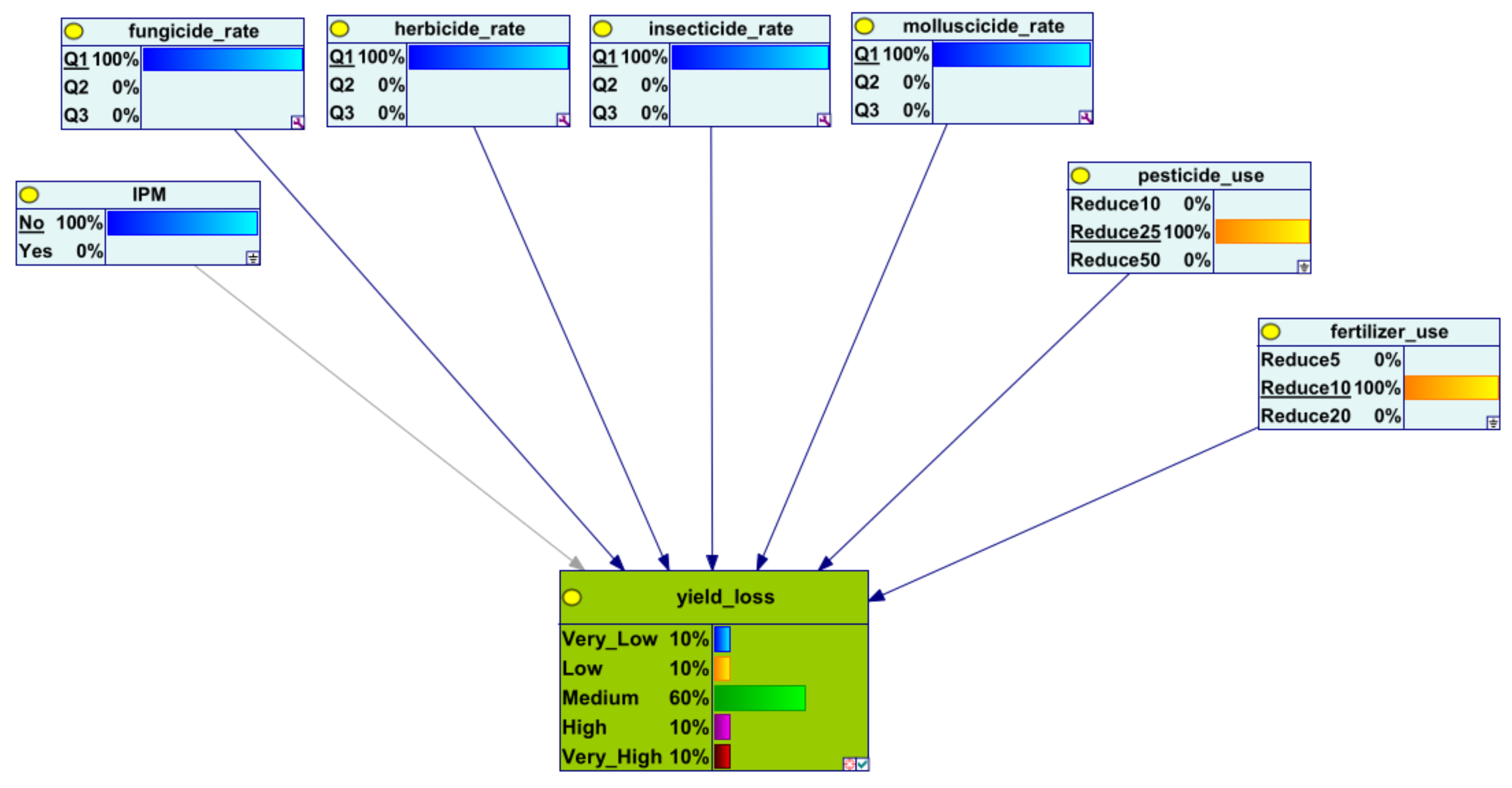
| 2 | No | 25 | 5 | 10 | 60 | 10 | 10 | 10 |
| 2 | No | 25 | 10 | 10 | 10 | 60 | 10 | 10 |
| 2 | No | 25 | 20 | 10 | 10 | 10 | 60 | 10 |
| 2 | No | 50 | 5 | 10 | 10 | 60 | 10 | 10 |
| 2 | No | 50 | 10 | 10 | 10 | 10 | 60 | 10 |
| 2 | No | 50 | 20 | 10 | 10 | 10 | 10 | 60 |
| 2 | Yes | 10 | 5 | 60 | 10 | 10 | 10 | 10 |
| 2 | Yes | 10 | 10 | 10 | 60 | 10 | 10 | 10 |
| 2 | Yes | 10 | 20 | 10 | 10 | 60 | 10 | 10 |
| 2 | Yes | 25 | 5 | 10 | 60 | 10 | 10 | 10 |
| 2 | Yes | 25 | 10 | 10 | 10 | 60 | 10 | 10 |
| 2 | Yes | 25 | 20 | 10 | 10 | 10 | 60 | 10 |
| 2 | Yes | 50 | 5 | 10 | 10 | 60 | 10 | 10 |
| 2 | Yes | 50 | 10 | 10 | 10 | 10 | 60 | 10 |
| 2 | Yes | 50 | 20 | 10 | 10 | 10 | 10 | 60 |
| % Reduction | Probability of Food Loss (%) | |||||||
|---|---|---|---|---|---|---|---|---|
| Q | IPM | Fertiliser | Pesticide | Very Low | Low | Medium | High | Very High |
| 3 | No | 10 | 5 | 60 | 10 | 10 | 10 | 10 |
| 3 | No | 10 | 10 | 10 | 60 | 10 | 10 | 10 |
| 3 | No | 10 | 20 | 10 | 10 | 60 | 10 | 10 |
| 3 | No | 25 | 5 | 10 | 60 | 10 | 10 | 10 |
| 3 | No | 25 | 10 | 10 | 10 | 60 | 10 | 10 |
| 3 | No | 25 | 20 | 10 | 10 | 10 | 60 | 10 |
| 3 | No | 50 | 5 | 10 | 10 | 60 | 10 | 10 |
| 3 | No | 50 | 10 | 10 | 10 | 10 | 60 | 10 |
| 3 | No | 50 | 20 | 10 | 10 | 10 | 10 | 60 |
| 3 | Yes | 10 | 5 | 60 | 10 | 10 | 10 | 10 |
| 3 | Yes | 10 | 10 | 10 | 60 | 10 | 10 | 10 |
| 3 | Yes | 10 | 20 | 10 | 10 | 60 | 10 | 10 |
| 3 | Yes | 25 | 5 | 10 | 60 | 10 | 10 | 10 |
| 3 | Yes | 25 | 10 | 10 | 10 | 60 | 10 | 10 |
| 3 | Yes | 25 | 20 | 10 | 10 | 10 | 60 | 10 |
| 3 | Yes | 50 | 5 | 10 | 10 | 60 | 10 | 10 |
| 3 | Yes | 50 | 10 | 10 | 10 | 10 | 60 | 10 |
| 3 | Yes | 50 | 20 | 10 | 10 | 10 | 10 | 60 |
Disclaimer/Publisher’s Note: The statements, opinions and data contained in all publications are solely those of the individual author(s) and contributor(s) and not of MDPI and/or the editor(s). MDPI and/or the editor(s) disclaim responsibility for any injury to people or property resulting from any ideas, methods, instructions or products referred to in the content. |
© 2024 by the authors. Licensee MDPI, Basel, Switzerland. This article is an open access article distributed under the terms and conditions of the Creative Commons Attribution (CC BY) license (https://creativecommons.org/licenses/by/4.0/).
Share and Cite
Barons, M.J.; Walsh, L.E.; Salakpi, E.E.; Nichols, L. A Decision Support System for Sustainable Agriculture and Food Loss Reduction under Uncertain Agricultural Policy Frameworks. Agriculture 2024, 14, 458. https://doi.org/10.3390/agriculture14030458
Barons MJ, Walsh LE, Salakpi EE, Nichols L. A Decision Support System for Sustainable Agriculture and Food Loss Reduction under Uncertain Agricultural Policy Frameworks. Agriculture. 2024; 14(3):458. https://doi.org/10.3390/agriculture14030458
Chicago/Turabian StyleBarons, Martine J., Lael E. Walsh, Edward E. Salakpi, and Linda Nichols. 2024. "A Decision Support System for Sustainable Agriculture and Food Loss Reduction under Uncertain Agricultural Policy Frameworks" Agriculture 14, no. 3: 458. https://doi.org/10.3390/agriculture14030458