
Research on Differential Steering Dynamics Control of Four-Wheel Independent Drive Electric Tractor


Abstract
:1. Introduction
2. Materials and Methods
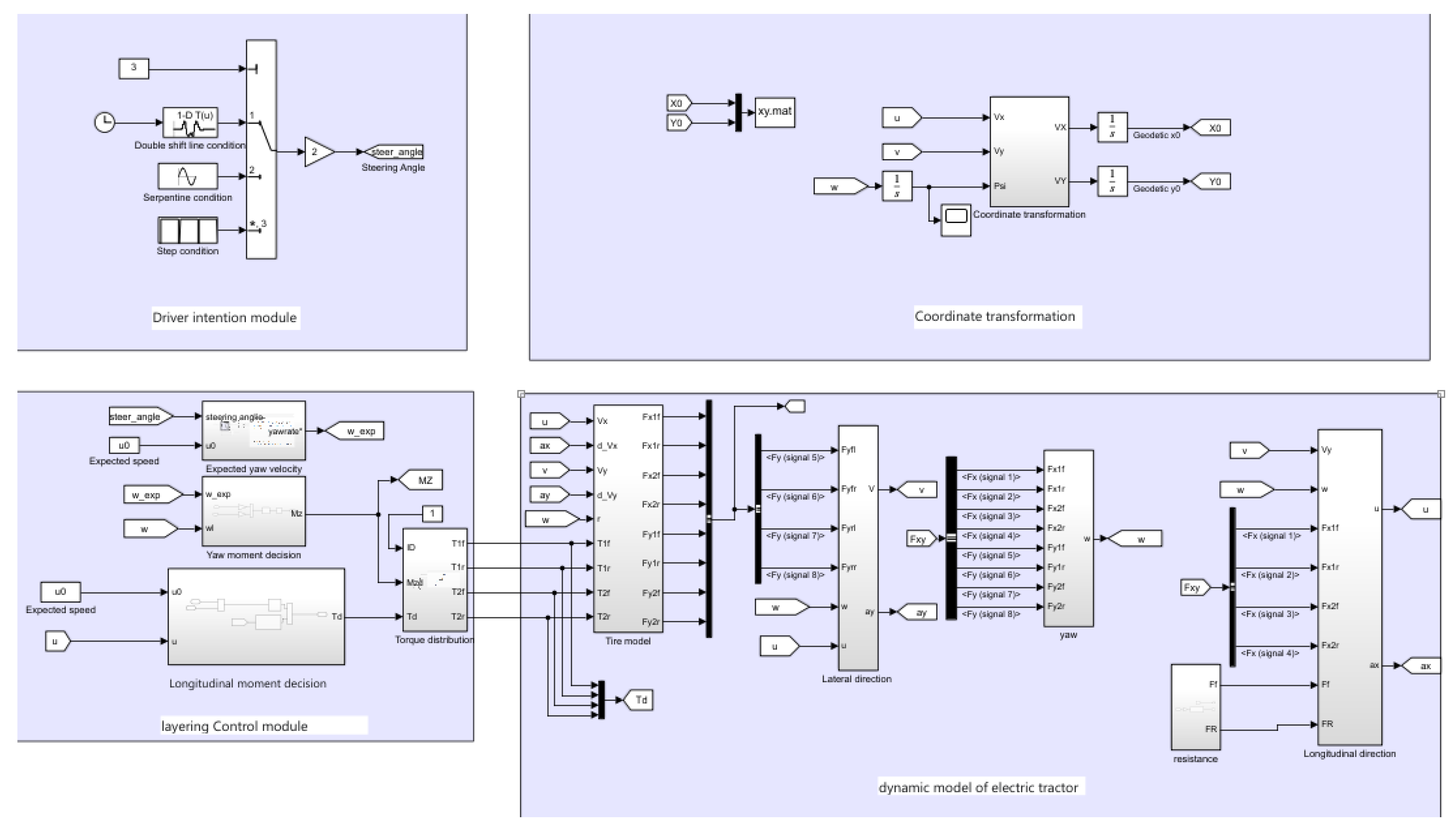
2.1. Establishment of Dynamic Model of Electric Tractor
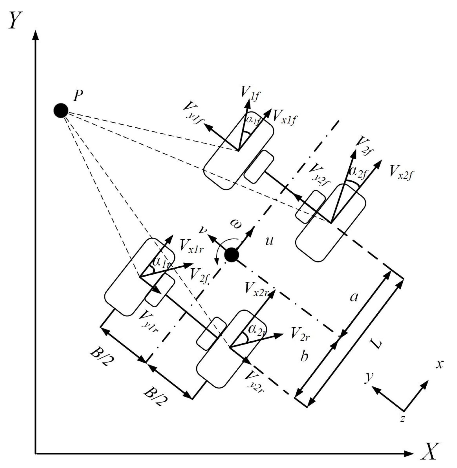
2.1.1. Tire Force Model
- (1)
- The longitudinal velocity at the center of gravity is constant;
- (2)
- When driving in a non-limiting state, the electric tractor is in a linear state, where it is assumed that the tire is in a linear region;
- (3)
- The electric tractor is driving on the horizontal road surface, and the center of gravity does not shift;
- (4)
- The air resistance faced by the vehicle at low speed is small and, thus, ignored in this paper.
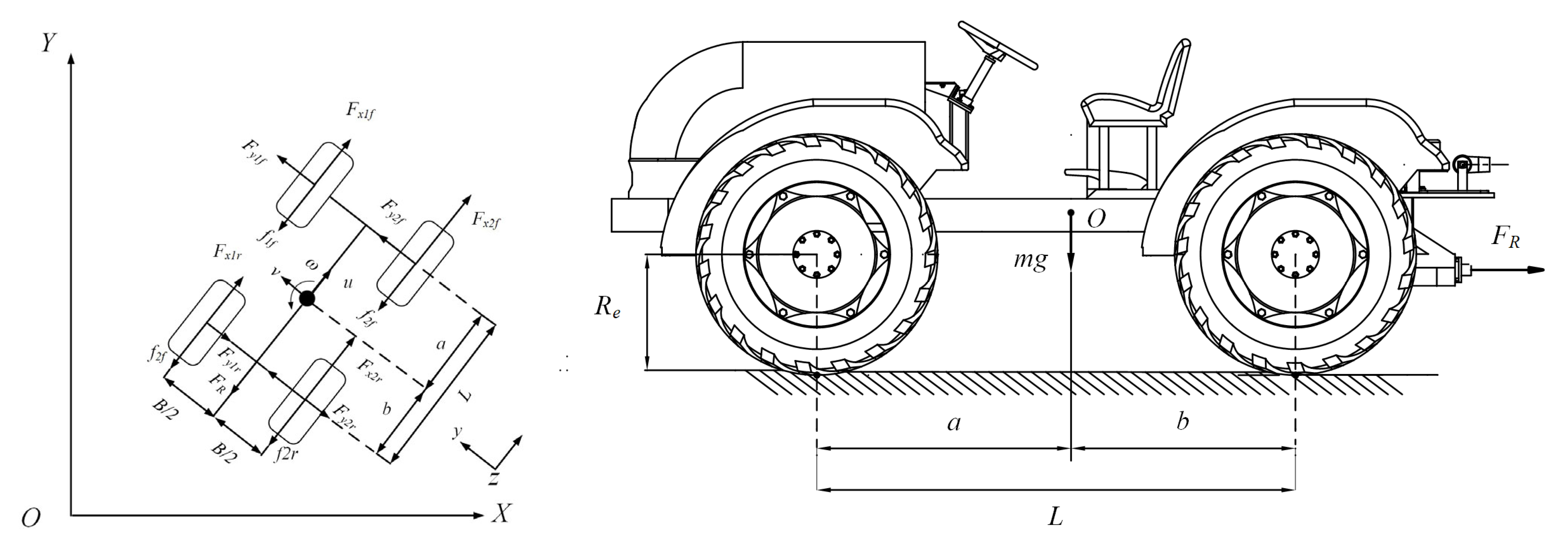
2.1.2. Body Dynamics Model
2.2. Driver Intention Recognition
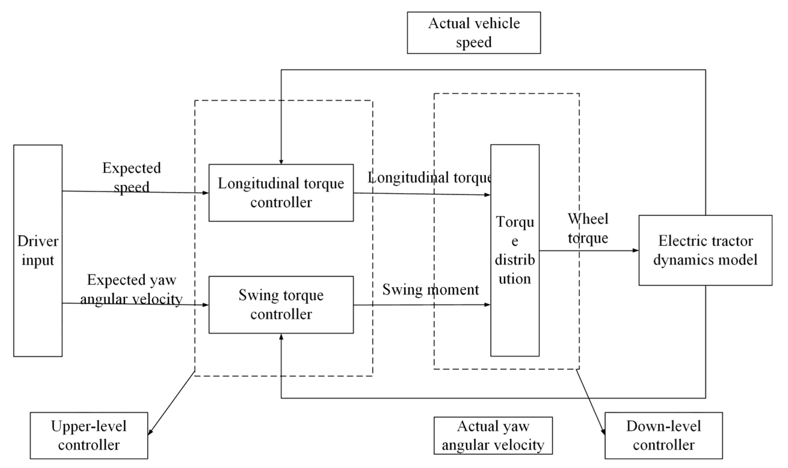
2.3. Layered Control Strategy for Differential Steering of Electric Tractor
2.3.1. Upper-Level Yaw Moment Setting Controller
2.3.2. Lower-Level Torque Distribution Controller
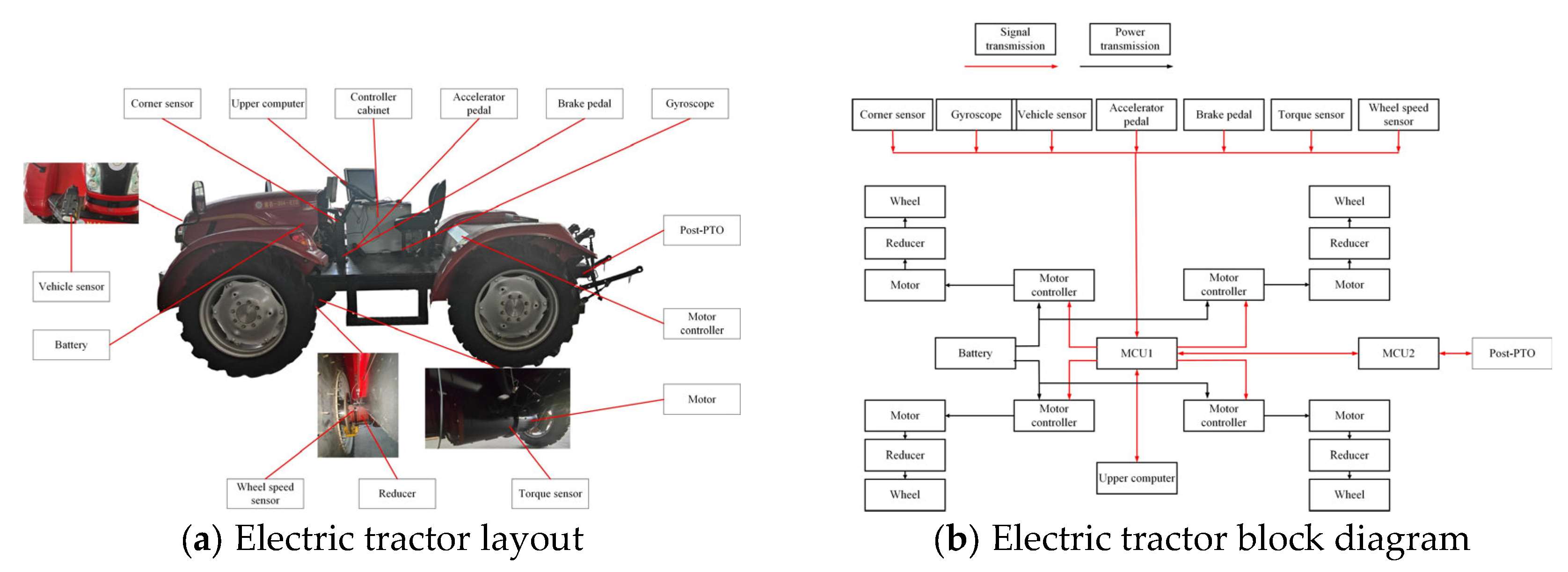
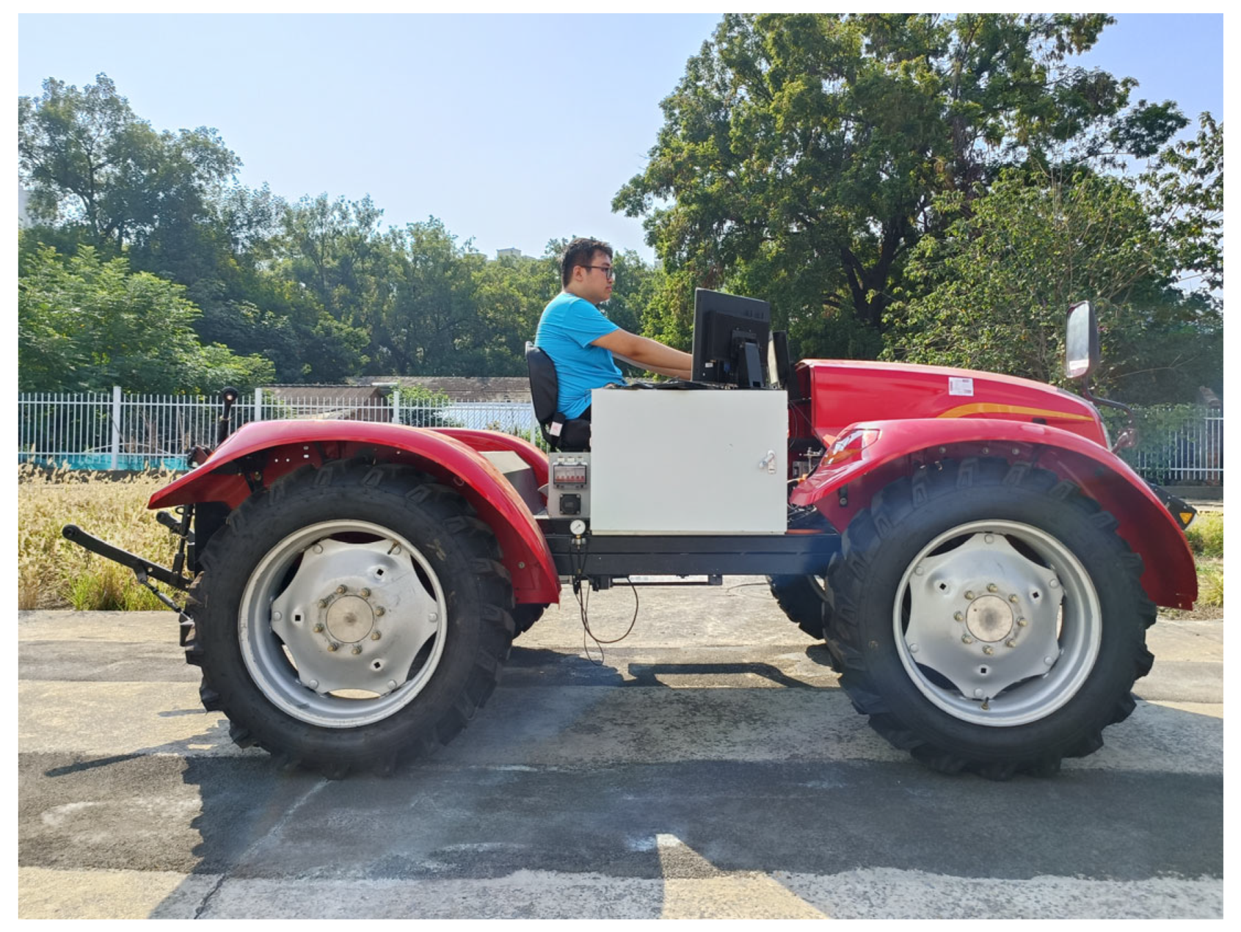
2.4. Real Electric Tractor
3. Results and Discussion
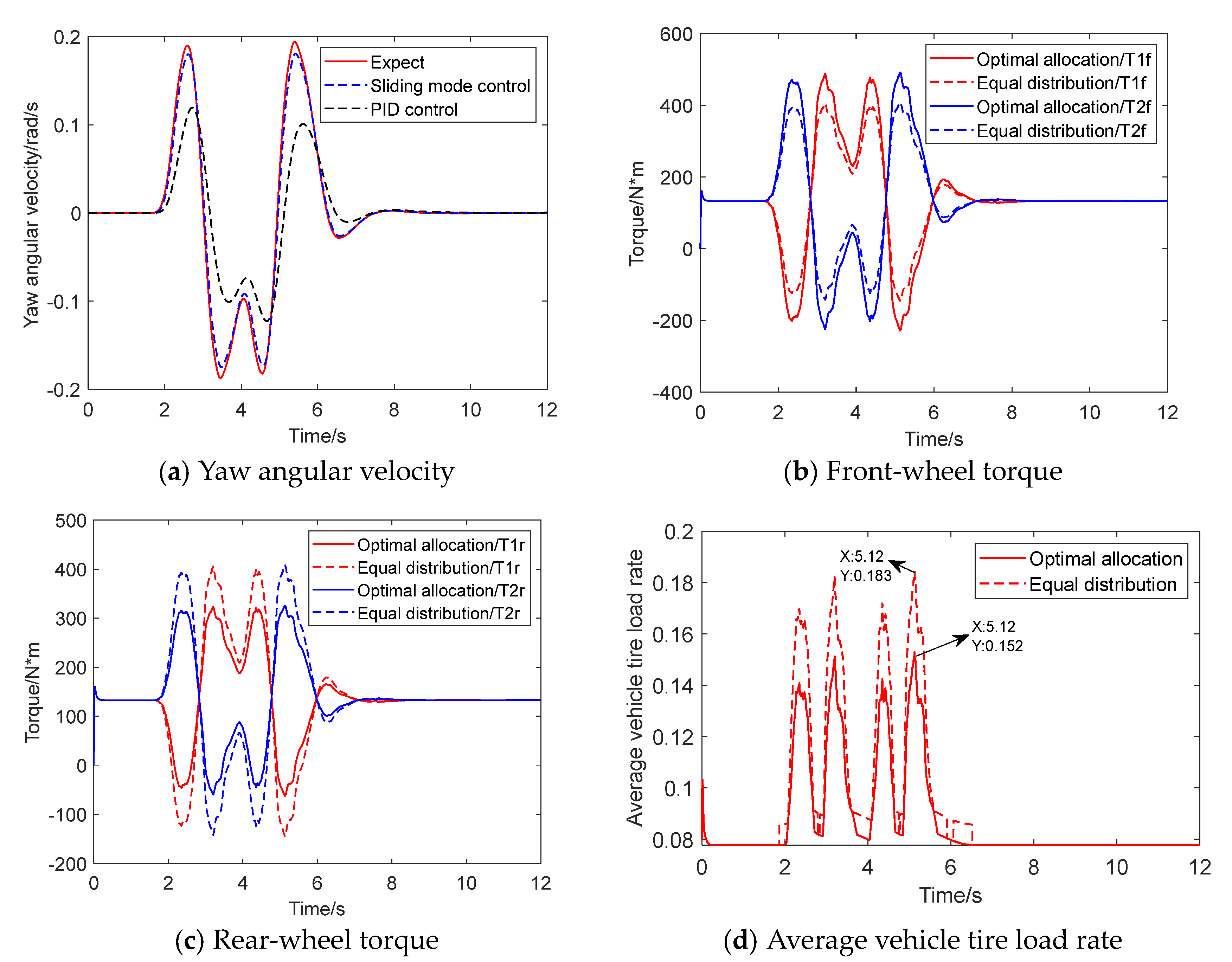
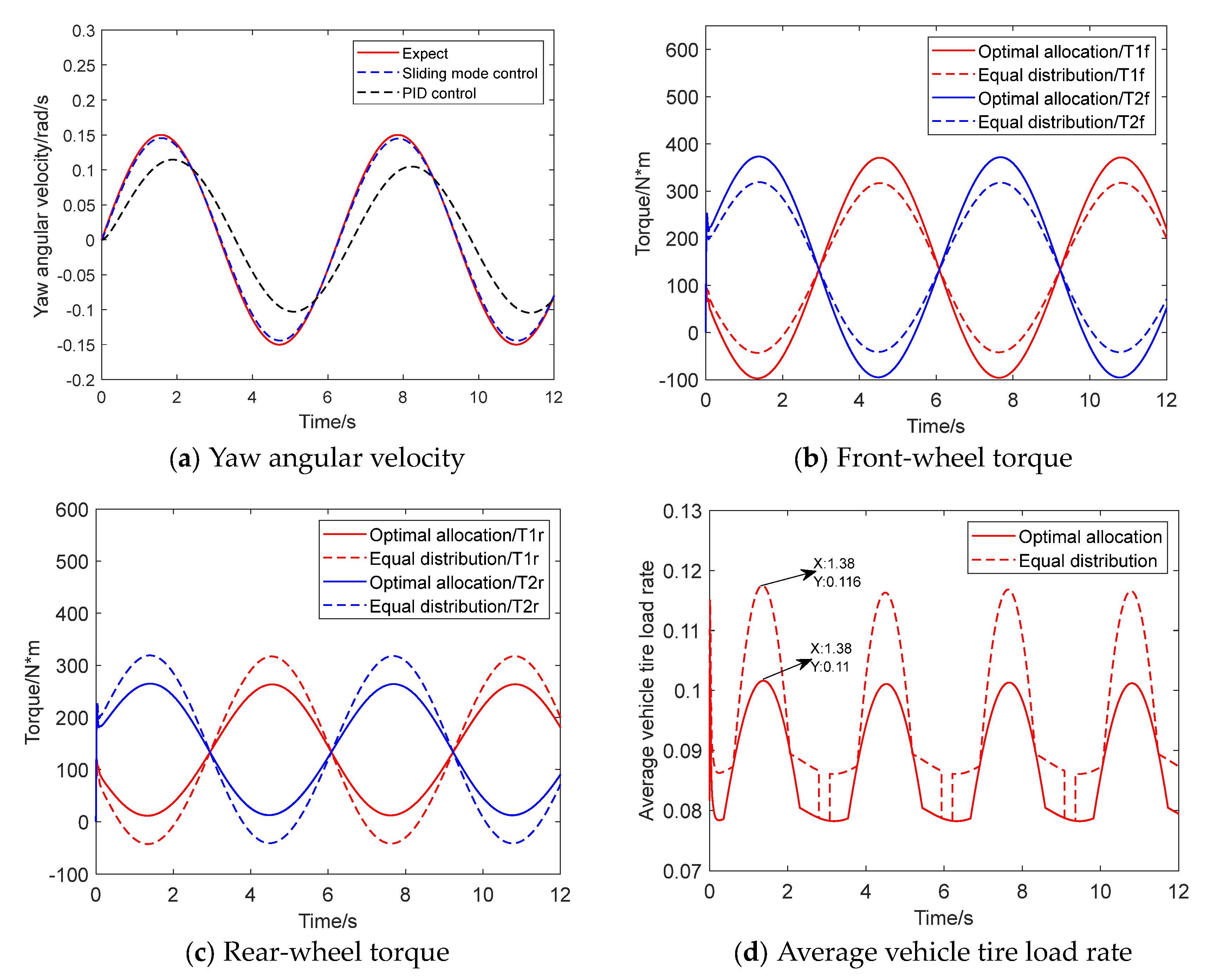
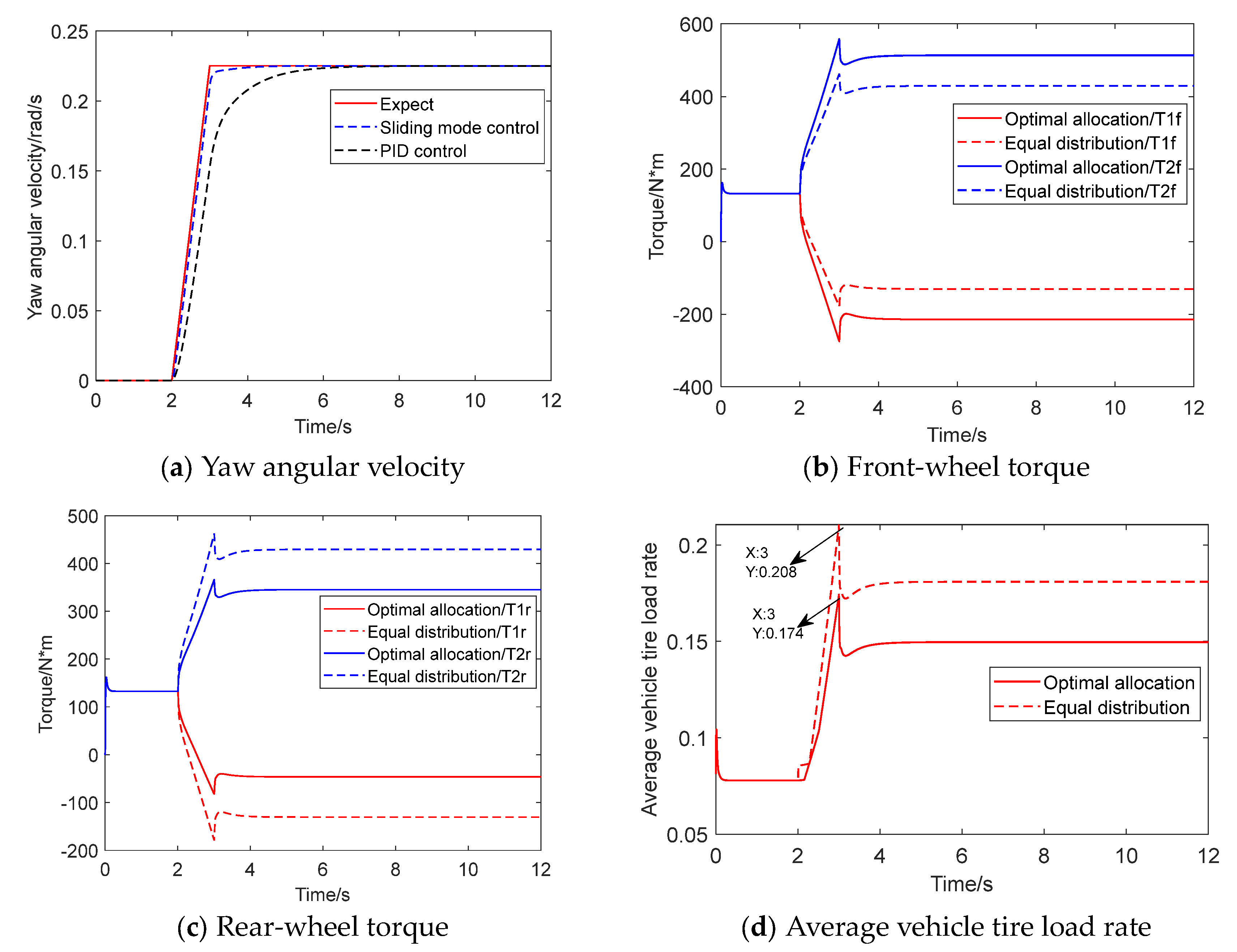
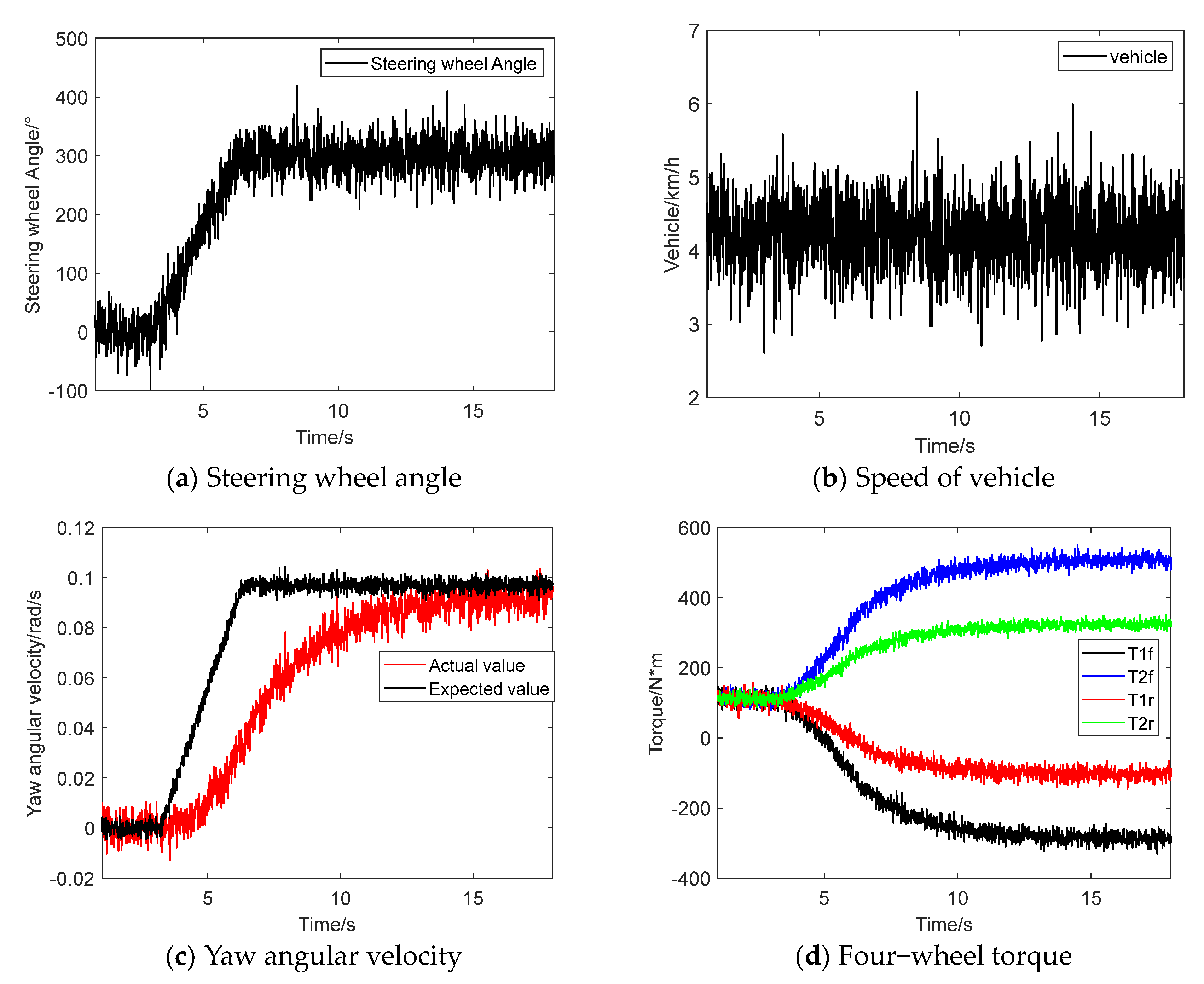
3.1. Simulation Experiment
- a.
- Double line shift condition
- b.
- Serpentine condition
- c.
- Step condition
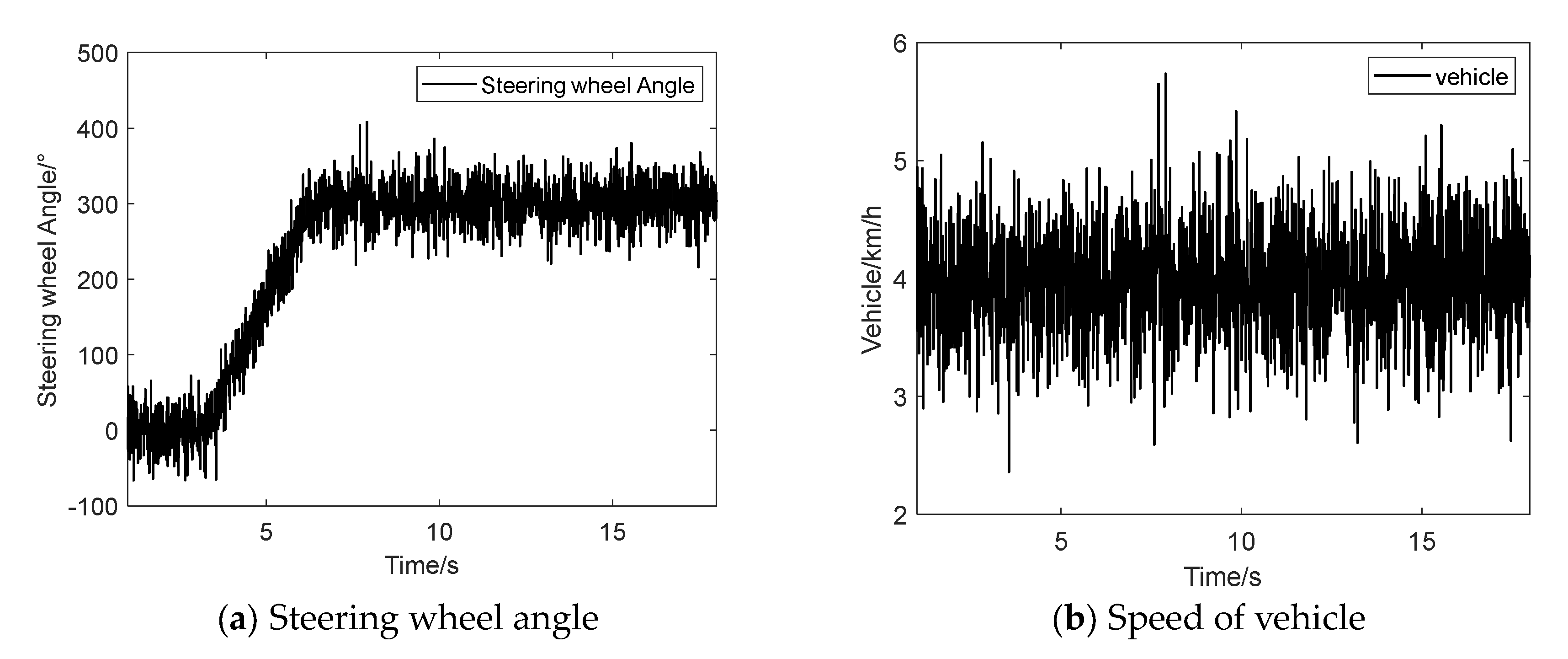
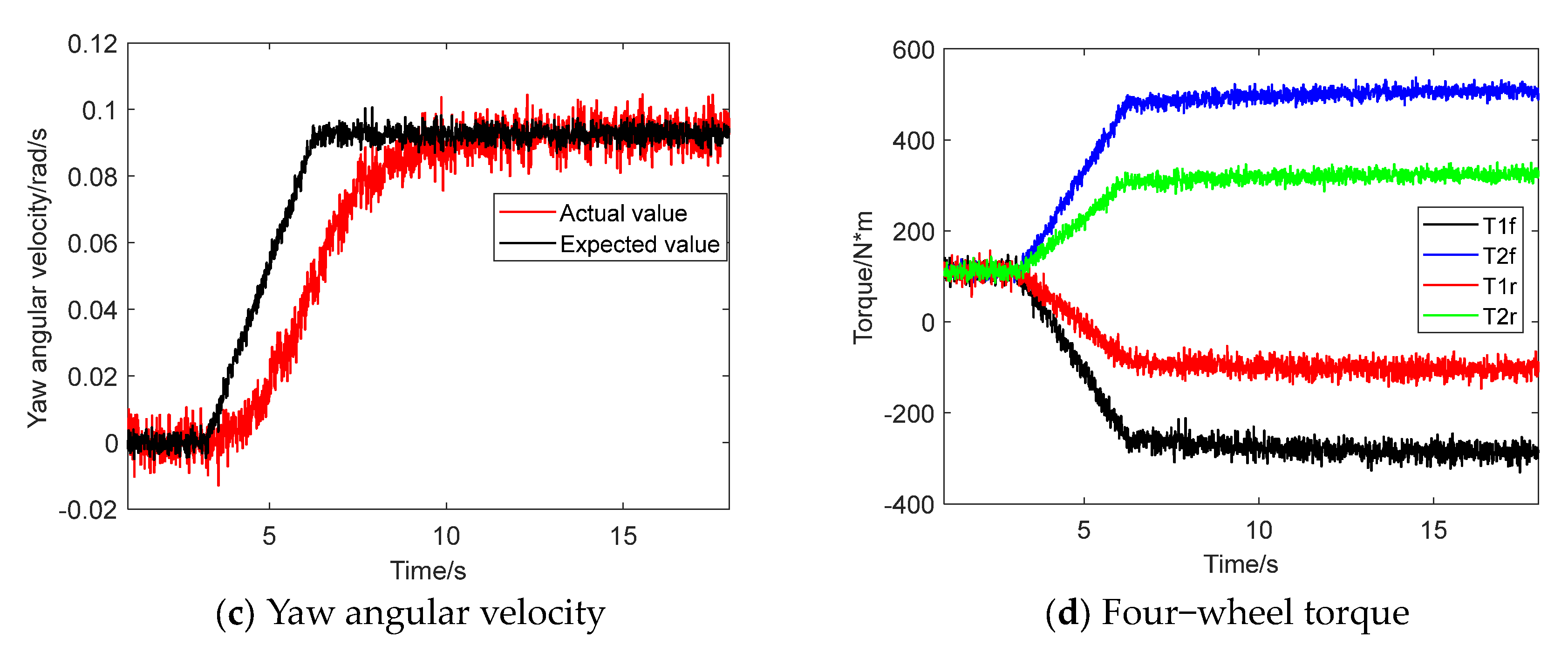
3.2. Car Test
4. Conclusions
Author Contributions
Funding
Institutional Review Board Statement
Data Availability Statement
Acknowledgments
Conflicts of Interest
References
- Liu, M.N.; Lei, S.H.; Zhao, J.H.; Meng, Z.J.; Zhao, C.J.; Xu, L.Y. Review on development and Research Status of Electric Tractor. Trans. Chin. Soc. Agric. Mach. 2022, 53, 348–364. [Google Scholar]
- Xie, B.; Wu, Z.B.; Mao, E.R. Development and the prospect of key technologies on agricultural tractor. Trans. Chin. Soc. Agric. Mach. 2018, 49, 1–17. [Google Scholar]
- Oscar, L.; Gunnar, L.; Anders, L.; Per-Anders, H. Impact of lowered vehicle weight of electric autonomous tractors in a systems perspective. Smart Agric. Technol. 2023, 4, 100156. [Google Scholar]
- Li, Z.C.; Li, J.Q.; Yang, S. The study on Differential Steering Control of In-wheel Motor Vehicle Based on Double Closed Loop System. En. Proc. 2018, 152, 586–592. [Google Scholar] [CrossRef]
- Fernandez, B.; Herrera, P.J.; Cerrada, J. Robust digital control for autonomous skid-steered agricultural robots. Comput. Electron. Agric. 2018, 153, 94–101. [Google Scholar] [CrossRef]
- Cao, F.Y.; Zhou, Z.L.; Zhao, J.H. Design of Steering Wheel Control System of Tracked Vehicle of Hydro-Mechanical Differential Turning. Adv. Mater. Res. 2012, 1671, 472–475. [Google Scholar] [CrossRef]
- Maclaurin, B. A skid steering model with track pad flexibility. J. Terramech. 2007, 44, 95–110. [Google Scholar] [CrossRef]
- Maclaurin, B. A skid steering model using the Magic Formula. J. Terramech. 2011, 48, 247–263. [Google Scholar] [CrossRef]
- Maclaurin, B. Comparing the steering performance of skid and Ackermann-steered vehicles. Proc. Inst. Mech. Eng. D J. Automob. Eng. 2008, 222, 739–756. [Google Scholar] [CrossRef]
- Yu, W.; Chuy, O.Y.; Collins, E.G.; Hollis, P. Analysis and experimental verification for dynamic modeling of a skid-steered wheeled vehicle. IEEE Trans. Robot. 2010, 26, 340–353. [Google Scholar] [CrossRef]
- Mokhiamar, O.; Amine, S. Lateral motion control of skid steering vehicles using full drive-by-wire system. J. Alex Eng. 2017, 56, 383–394. [Google Scholar] [CrossRef]
- Du, P.; Ma, Z.M.; Chen, H.; Xu, D.; Wang, Y.; Jiang, Y.H.; Lian, X.M. Speed-adaptive motion control algorithm for differential steering vehicle. Proc. Inst. Mech. Eng. D J. Automob. Eng. 2021, 235, 672–685. [Google Scholar] [CrossRef]
- Ni, J.; Hu, J.; Xiang, C. Robust path following control at driving handling limits of an autonomous electric racecar. IEEE Trans. Veh. Technol. 2019, 68, 5518–5526. [Google Scholar] [CrossRef]
- Shino, M.; Nagai, M. Independent wheel torque control of small-scale electric vehicle for handling and stability improvement. JSAE Rev. 2003, 24, 449–456. [Google Scholar] [CrossRef]
- Xu, D.; Wang, G.D.; Cao, B.G.; Feng, X.H. Research on torque optimal allocation strategy of independent drive electric vehicle. J. Xian Jiao Tong Univ. 2012, 46, 42–46. [Google Scholar]
- Li, Q.W.; Zhang, H.H.; Yan, S.; Gao, C. Single wheel failure stability control for four-wheel independent drive electric vehicles. Control Eng. 2021, 28, 155–163. [Google Scholar]
- Yan, Y.B.; Zhang, Y.N.; Yan, N.M.; Han, B.L. Simulation Research on motion control algorithm of six wheel independent drive sliding steering vehicle. J. Ordnance Ind. 2013, 34, 1461–1468. [Google Scholar]
- Kang, J.; Kim, W.; Lee, J.; Yi, K. Skid steering-based control of a robotic vehicle with six in-wheel drives. Proc. Inst. Mech. Eng. D J. Automob. Eng. 2010, 224, 1369–1391. [Google Scholar] [CrossRef]
- Lu, Y.J.; Yang, S.P.; Li, S.H. Research on dynamics of a class of heavy vehicle-tire-road coupling system. Sci. Sci. China Technol. Sci. 2011, 54, 2054–2063. [Google Scholar] [CrossRef]
- Li, Y.X.; Wang, Y.C.; Feng, P.F. Lateral Dynamics of Three-axle Steering Vehicle Based Zero Vehicle Sideslip Angle Control. New Mater. New Process. 2012, 476, 1682–1687. [Google Scholar] [CrossRef]
- Rezaeian, A.; Zarringhalam, R.; Fallah, S.; Melek, W.; Khajepour, A.; Chen, S.K.; Moshchuck, N.; Litkouhi, B. Novel Tire Force Estimation Strategy for Real-Time Implementation on Vehicle Applications. Trans. Vehicle Tec. 2015, 64, 2231–2241. [Google Scholar] [CrossRef]
- Xiong, L.; Huang, S.S.; Chen, Y.L.; Yang, G.X.; Zhang, R. Research on motion tracking control of wheeled differential steering unmanned vehicle. Auto. Eng. 2015, 37, 1109–1116. [Google Scholar]
- Yu, Z.P.; Gao, L.T.; Zhang, R.X.; Xiong, L. Wheel motor drives differential steering vehicle dynamics control. J. Tongji Univ. Nat. Sci. 2018, 46, 631–638. [Google Scholar]
- Cho, J.; Huh, K. Active Front Steering for Driver’s Steering Comfort and Vehicle Driving Stability. Int. J. Auto. Technol. 2019, 20, 589–596. [Google Scholar] [CrossRef]
- Jeong, D.; Kim, S.T.; Choi, S.B.; Kim, M.; Lee, H.J. Estimation of Tire Load and Vehicle Parameters Using Intelligent Tires Combined With Vehicle Dynamics. IEEE Trans. Instrum. Meas. 2018, 70, 101109. [Google Scholar] [CrossRef]
- Grecenko, A.; Prikner, P. Tire rating based on soil compaction capacity. J. Terramech. 2014, 52, 77–92. [Google Scholar] [CrossRef]
- Liu, J.; Sun, F. Research and Progress of Sliding Mode Variable Structure Control Theory and its Algorithms. Control. Theory Appl. 2007, 24, 407–418. [Google Scholar]
- Wu, D.M.; Li, Y.; Zhang, J.W.; Du, C.Q. Torque distribution of a four in-wheel motors electric vehicle based on a PMSM system model. Proc. Inst. Mech. Eng. D J. Automob. Eng. 2018, 232, 1828–1845. [Google Scholar] [CrossRef]


| Name | Argument | Numerical Value | Unit |
|---|---|---|---|
| Total tractor mass | 2105 | kg | |
| Tractor wheelbase | 2.05 | m | |
| Distance from center of mass to front axis | 0.82 | m | |
| Distance from center of mass to rear axis | 1.23 | m | |
| Tractor wheel gauge | 2.12 | m | |
| Principal moment of inertia around the z-axis | 2537 | kg·m2 | |
| Wheel radius | 0.53 | m | |
| Wheel inertia | 11.52 | kg·m2 |
Disclaimer/Publisher’s Note: The statements, opinions and data contained in all publications are solely those of the individual author(s) and contributor(s) and not of MDPI and/or the editor(s). MDPI and/or the editor(s) disclaim responsibility for any injury to people or property resulting from any ideas, methods, instructions or products referred to in the content. |
© 2023 by the authors. Licensee MDPI, Basel, Switzerland. This article is an open access article distributed under the terms and conditions of the Creative Commons Attribution (CC BY) license (https://creativecommons.org/licenses/by/4.0/).
Share and Cite
An, Y.; Wang, L.; Deng, X.; Chen, H.; Lu, Z.; Wang, T. Research on Differential Steering Dynamics Control of Four-Wheel Independent Drive Electric Tractor. Agriculture 2023, 13, 1758. https://doi.org/10.3390/agriculture13091758
An Y, Wang L, Deng X, Chen H, Lu Z, Wang T. Research on Differential Steering Dynamics Control of Four-Wheel Independent Drive Electric Tractor. Agriculture. 2023; 13(9):1758. https://doi.org/10.3390/agriculture13091758
Chicago/Turabian StyleAn, Yuhui, Lin Wang, Xiaoting Deng, Hao Chen, Zhixiong Lu, and Tao Wang. 2023. "Research on Differential Steering Dynamics Control of Four-Wheel Independent Drive Electric Tractor" Agriculture 13, no. 9: 1758. https://doi.org/10.3390/agriculture13091758