Article

Unmanned Aerial System-Based Wheat Biomass Estimation Using Multispectral, Structural and Meteorological Data

1
College of Earth Science, Chengdu University of Technology, Chengdu 610059, China
2
College of Geoscience and Surveying Engineering, China University of Mining and Technology (Beijing), Beijing 100083, China
3
School of Environment and Spatial Informatics, China University of Mining and Technology, Xuzhou 221116, China
4
Department of Land Management, Zhejiang University, Hangzhou 310058, China
*
Author to whom correspondence should be addressed.
Agriculture 2023, 13(8), 1621; https://doi.org/10.3390/agriculture13081621
Submission received: 10 June 2023 / Revised: 21 July 2023 / Accepted: 26 July 2023 / Published: 17 August 2023
(This article belongs to the Special Issue Remote Sensing Technologies in Agricultural Crop and Soil Monitoring)

Abstract

:
Rapid estimation of above-ground biomass (AGB) with high accuracy is essential for monitoring crop growth status and predicting crop yield. Recently, remote sensing techniques using unmanned aerial systems (UASs) have exhibited great potential in obtaining structural information about crops and identifying spatial heterogeneity. However, methods of data fusion of different factors still need to be explored in order to enhance the accuracy of their estimates. Therefore, the objective of this study was to investigate the combined metrics of different variables (spectral, structural and meteorological factors) for AGB estimation of wheat using UAS multispectral data. UAS images were captured on two selected growing dates at a typical reclaimed cropland in the North China Plain. The spectral response was determined using the highly correlated vegetation index (VI). A structural metric, the canopy height model (CHM), was produced using UAS-based multispectral images. The measure of growing degree days (GDD) was selected as a meteorological proxy. Subsequently, a structurally–meteorologically weighted canopy spectral response metric (SM-CSRM) was derived by the pixel-level fusion of CHM, GDD and VI. Both correlation coefficient analysis and simple function fitting were implemented to explore the highest correlation between the measured AGB and each proposed metric. The optimal regression model was built for AGB prediction using leave-one-out cross-validation. The results showed that the proposed SM-CSRM generally improved the correlation between wheat AGB and various VIs and can be used for estimating the wheat AGB. Specifically, the combination of MERIS terrestrial chlorophyll index (MTCI), vegetation-masked CHM (mCHM) and normalized GDD (nGDD) achieved an optimal accuracy (R2 = 0.8069, RMSE = 0.1667 kg/m2, nRMSE = 19.62%) through the polynomial regression method. This improved the nRMSE by 3.44% compared to the predictor using MTCI × mCHM. Moreover, the pixel-level fusion method slightly enhanced the nRMSE by ~0.3% for predicted accuracy compared to the feature-level fusion method. In conclusion, this paper demonstrated that an SM-CSRM using pixel-level fusion with canopy spectral, structural and meteorological factors can obtain a good level of accuracy for wheat biomass prediction. This finding could benefit the assessment of reclaimed cropland or the monitoring of crop growth and field management in precision agriculture.

1. Introduction

Crops are extremely important for human beings. The monitoring of crop growth is essential for precision agriculture or cropland reclamation, helping to understand the physiological status of crops, forecast the agricultural production [1], and evaluate reclaimed cropland. Various crop traits can be monitored to reflect the crop’s response to the growing environment and management practices [2], such as above-ground biomass (AGB) [3] and canopy chlorophyll content (CCC) [4]. These indicators are closely related to light use efficiency and grain quality [5]. Therefore, rapid and accurate estimation of crop parameters is beneficial for field management tasks, such as pest control [6], fertilizer measurement [7], and yield prediction. In particular, wheat (Triticum aestivum) is one of the most important food crops, with a long history. Globally, it has the largest cultivated area and highest production levels among all crops, including corn and rice [8]. Moreover, wheat is also a typical ridge-cultivated crop. Hence, improving the estimation of wheat AGB is a significant objective.
Methods of estimating the AGB of crops have been extensively reported. Conventionally, a destructive method is employed by harvesting and drying the stems and leaves of crops above the ground in a sampling plot. It is time-consuming, labor-intensive and inefficient to operate on a large-scale site. Currently, remote sensing-based techniques have been given more and more attention in predicting the AGB of crops at numerous spatial scales [9,10]. These techniques can capture multi-temporal data of crops in a large area via non-destructive methods at a relatively low cost. Different observation platforms, including space-borne [9], airborne [11], unmanned aircraft systems (UASs) [12] or ground-based platforms mounted with diverse sensors, such as optical [13], multispectral [9], hyperspectral [12] or light detection and ranging (LiDAR) sensors [11], have been used in biomass predictions. Space-borne platforms observe the field on a large scale, but they are easily blocked by adverse weather conditions. Airborne platforms can be restricted by takeoff and landing conditions. Ground-based observations can capture fine images but can hardly be used to obtain wall-to-wall data. UAS-based platforms provide data with high spatial, spectral and temporal resolution, exhibiting great potential in precision agriculture [14] or other related applications.
Recently, UAS-based methods have been extensively introduced into the quantitative retrieval of crop parameters because of their advantages in identifying spatial heterogeneity and ability to obtain crop structural information. On the one hand, numerous variables have been discussed that have the potential to improve estimates of crop AGB using UAS remote sensing observations, including canopy spectral signatures, structural features, textural characteristics and climatic factors [10]. Spectral information is a widely used indicator for estimating the AGB of crops. A large number of vegetation indices have been explored and the most highly correlated indices have been selected for use in biomass prediction, such as the green–red ratio index (GRRI) derived from RGB imagery [13], normalized difference red-edge index (NDRE) produced from multispectral images [15], or modified chlorophyll absorption reflectance index (MCARI) derived from hyperspectral data [16]. Structure features determine the canopy shape of crops, including crop height, the coefficient of variation for plant height, etc. These structural indicators are significant for addressing the spectral saturation problem [17]. Textural characteristics are relevant to the distribution of both vegetation and soil pixels across canopy surfaces, which accounts for the spatial variation of dark and bright areas on images. These proxies have been demonstrated to be significantly associated with the AGB of crops in the breeding experimental field [18]. Moreover, climatic factors are useful in conventional predictions of crop biomass when combined with satellite images of large-scale regions in the main maize cultivation areas of China [19]. Recent studies have also demonstrated the effectiveness of using climatic factors to improve the predicted accuracy of crop biomass on a small scale, such as in a commercial maize field of 18.02 ha in southeastern Spain [20] and a rice field of 0.27 ha at the experimental base of hybrid rice in Lingshui in southern China [15]. Growing degree days (GDD) is an effective indicator, measures the effective accumulated heat over a certain temperature throughout crop growth, and has a close correlation with crop AGB [15]. It can be regarded as an independent variable that can improve the accuracy of biomass prediction [21]. On the other hand, a combination of these factors can improve the accuracy of AGB prediction [13,20]. Previous studies have confirmed that different strategies of data fusion yield varying abilities of crop biomass estimation, including pixel-level, feature-level, or even decision-level data fusion. In fact, image fusion at the feature level or pixel level is generally adopted in order to estimate crop biomass. Examples of this practice include pixel-level fusion, combining the vegetation index weighted canopy volume model (CVMVI) for soybean [13], and feature-level fusion, integrating the canopy multispectral information, crop height and meteorological factors for rice [15]. It has been proved that the pixel-level strategy can achieve a slightly higher accuracy than that obtained with the feature-level fusion of soybean [13]. Besides, multispectral sensors usually include bands with sensitivity to vegetation growth status, such as red-edge and near-infrared bands, in order to record the detailed canopy response [22]. However, the appropriate method for combining these data still needs further exploration in order to improve the accuracy of biomass prediction.
Previous studies present a research gap in terms of integrating the different factors in pixel-level data fusion to predict crop biomass. Therefore, the objective of this paper is to investigate the combination of discussed variables in order to improve the accuracy of AGB estimation. The specific goals are to (1) propose a metric for combining variables in pixel-level fusion as a predictor of wheat AGB, considering spectral, structural, meteorological factors, and (2) to explore the optimal estimation model of wheat biomass, using the proposed metric as the predictor.

2. Materials and Methods

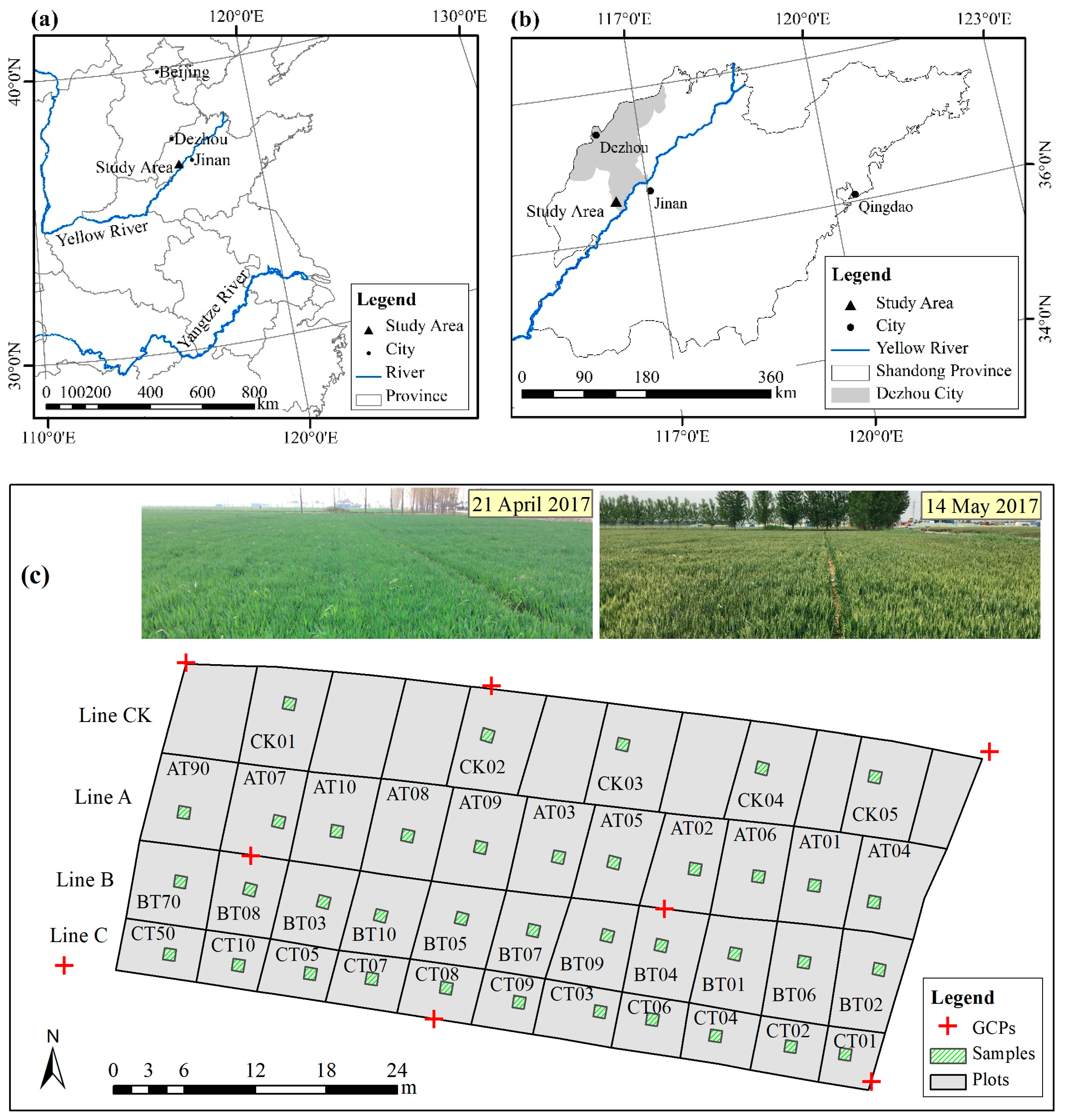
2.1. Study Area and Experimental Designing

The study area was located around 60 km in the west of Jinan, Shandong Province of China (36°28′21″ N, 116°28′08″ E). This region experiences an average annual rainfall of 556.9 mm and an average annual temperature of 14.5 °C. It is a representative agricultural landscape of the North China Plain (NCP), with a typical temperate monsoon climate. The NCP is a crucial agricultural zone in China and produces over 75% and 32% of Chinese wheat and corn, respectively [23].
The experimental field was approximately 1200 m2 in size, with an average elevation 28.98 m. The soil type was identified as silty loam, with a pH value of 8.1 and an organic content of around 8.5 g/kg. The site was located in the NCP (see Figure 1a,b) and was created by farmland reclamation activities due to ground subsidence induced by underground coal exploitation. In total, 38 plots were distributed throughout the experimental field (see Figure 1c). Diverse soil profiles were designed to adopt inter-layers of filling materials, including local soil and sediments from the Yellow River with different thicknesses. A total of 13 inter-layer soil profiles and 1 control profile were constructed (see Figure 2 for detailed design). This field represents a collection of various refilling profiles, making it a typical reclaimed cropland in practice. For instance, the profile of T09 consists of a 30 cm topsoil layer, followed by a 20 cm subsoil layer, a 20 cm layer of sediment from the Yellow River, another 20 cm of subsoil layer, and a final 30 cm layer of sediment from the Yellow River at the bottom.

2.2. Data Acquisition

2.2.1. UAS Platform and Data Acquisition

The UAS platform employed was DJI Matrice 100 (see Figure 3). This is a low-cost and high-stability platform with a maximum hovering duration of 20 min and a 500 g payload. The platform is equipped with an onboard flight controller that incorporates various modules, including a compass, barometer, inertial measurement unit (IMU) and global positioning system (GPS). The flight route can be preplanned and transmitted to the control system of the platform. This allows the UAS to follow a predetermined trajectory at the desired altitude during the flight.
The multispectral camera used was a Parrot Sequoia (see Figure 3) with a focal length 3.98 mm. It comprised two parts: the multispectral sensor (72 g), containing four bands (green: 530–570 nm; red: 640–680 nm; red-edge: 730–740 nm; and near-infrared: 770–810 nm) at a resolution of 1280 × 960 pixels, and the sunshine sensor (35 g), which was placed on the top of drone. The multispectral images were recorded on the built-in memory card of the multispectral sensor and could be accessed after flight mission. Sequoia can be triggered according to an equal distance or time interval. The time interval mode was adopted and set to three seconds in this paper. The sunshine sensor can continuously record the light conditions of the external environment, and the recorded data could then be employed in the radiometric correction of spectral signatures.
Multispectral images were obtained between 11:00 and 14:00 on two dates (23 April 2017, 14 May 2017) during crop growth. The flight mission was planned using the software DJI GS Pro. The flight altitude was set at 50 m, with a nominal ground sampling distance (GSD) of 4.7 cm. The side overlap was 80% and the forward overlap was 90%, providing sufficient image overlap for post-processing. The same flight route was used for both missions, ensuring flight consistency during data collection. Before each flight, a rectangular calibration panel provided by the manufacturer served as the standard reference for four-band reflectance. The panel was placed near the take-off and landing point, and a set of multispectral images were taken from the top of the panel at around a 1 m height for radiometric correction during post-processing.
Ground control points (GCPs) were employed to transform the system from a relative into an absolute coordinate system. Eight GCPs were distributed on the cropland ridges in the experimental field (see Figure 1c), and the targets were marked with crosses using lime. The coordinates of these points were measured using a global navigation satellite system (GNSS) receiver mentioned above.
To generate the point cloud and band reflectance map of the crop canopy, the collected multispectral images were imported into Pix4D mapper software (Pix4D SA, Lausanne, Switzerland), which integrates the principles of photogrammetry and computer vision to process the stereoscopic photos. The imagery was first processed using structure from motion (SfM), which includes feature extraction and matching to establish point correspondence. An iterative bundle adjustment was performed to estimate the 3D position of points, and a clustering view for multi-view stereo (CMVS) was used to densify the sparse point cloud. Additionally, GCPs were manually identified from the overlapping images for rectification into absolute coordinates. To produce the digital surface model (DSM), the dense point cloud was interpolated using inverse distance weighting (IDW), which was carried out in ArcMap 10.0 (ESRI, Redlands, CA, USA).

2.2.2. Crop Height and AGB Measurement

Field measurement included crop height and the weight of dry AGB. The sampling size was 1 m × 1 m, covering four rows of wheat, because of its row spacing of 25 cm. On the one hand, the crop height of 10 plants was measured in each sample using a steel tape. Measurements were taken one day before or after each UAS flight (23 April 2017 and 14 May 2017). Each plant was surveyed from the ground above the soil to its youngest and completely unfurled leaf. The mean height of these 10 plants served as the validation for the sampling plot. On the other hand, sampling plants were gathered from each sampling plot after each UAS flight. Ten stems were sampled and first dried for two hours at 105 °C to remove green, and then dried to a constant weight for over 24 h at 80 °C. Additionally, the total number of plants was counted in each sampling plot during field observation. Finally, the dry weight of AGB was realized in the unit of kg/m2 (see Equation (1)):
D A G B = 1 n d × N 1000
where d is the dry weight of 10 sampled plants, n is the sampling number of the wheat plant (10 plants in this study), and N is the total plants in the sampling plot.
Besides, the central coordinates of the sampling points were surveyed using a GNSS receiver (South Survey GALAXY G1, real-time kinematics surveying with a typical accuracy of 0.008 m + 1 ppm horizontally and 0.015 m + 1 ppm vertically).

2.2.3. Meteorological Data

Meteorological factors have conventionally been reported to be closely related to the accumulation of crop biomass, especially the effective accumulated temperature [20]. Hence, the meteorological data were collected from two adjacent regional-level weather stations in the east and west, located around 8 km from the study area. The collected items included maximum and minimum daily temperature from 1 October 2016, to 30 September 2017. These data were recorded by the local administrative bureau.

2.3. Method

This study first proposed a metric that combined structural and meteorological data with canopy spectral information using pixel-level data fusion, and secondly implemented AGB modelling and validation using the proposed highly correlated metric. The metric was referred to as the structurally–meteorologically weighted canopy spectral response metric (SM-CSRM). The workflow of this study can be seen in Figure 4.

2.3.1. Spectral, Structural and Metrological Indicators

(a) Selection of vegetation indices (VIs). VIs are indicators of canopy reflectance response. Previous studies have reported that VIs derived from UAS-based multispectral reflectance showed good performance in the prediction of crop parameters, such as above-ground biomass and crop yield [16,24]. Therefore, we chose 25 highly correlated VIs based on various reported studies in order to explore their correlation with measured wheat AGB. The equations for these VIs were listed in the Appendix A of Table A1.
(b) CHM generation and vegetation mask. Crop height contains the canopy structural information in the vertical direction and serves as a useful proxy for AGB prediction [13,15]. It helps to mitigate the saturation issue of spectral indices in response to changes in biomass with higher vegetation density [17,25]. The canopy height model (CHM) provides wall-to-wall data of crop height through UAS-based estimation. CHM has been widely tested using SfM-based methods, such as optical cameras or multispectral cameras. UAS-based multispectral images have been demonstrated to be a viable alternative for canopy height estimation in crops like wheat and corn [26]. Therefore, this study employed optimal settings to generate the CHM of wheat using UAS-based multispectral images. The general process is as follows: (1) produce dense the point cloud using a generating setting of 90,000 feature points; (2) filter the point cloud using statistical outlier removal (SOR) and conditional removal (CR); (3) obtain the DSM using IDW method; and (4) calculate the CHM by subtracting the DSM from the DEM. The specific parameters can be seen in the published literature [26].
Vegetation masks were considered to account for the spatial heterogeneity of the reclaimed farmland and were built using a supervised classification method of random forest (RF) with spectral band-derived VIs. RF is an ensemble learning algorithm that effectively addresses the issue of weak generalization ability observed in decision tree methods. The excellent performance of RF in image classification has been confirmed by many studies [27]. The specific steps were as follows: (1) 1000 sampling points were randomly generated within the study site using the GIS software and divided into two parts on the basis of training points (70%) and validation points (30%). The reference values were achieved via visual interpretation using the orthomosaic as a background. (2) The simple ratio (SR) was selected as the input for classification, and the RF classifier was selected as the classification method. (3) Kappa coefficient (KC) and overall accuracy (OA) were chosen as verification indicators after the classification. The classification results showed that KC was higher than 0.942 for each date and that OA was higher than 94.4%. Then, the vegetation masks of wheat were obtained for two observed images after the completion of these steps discussed above. Subsequently, a vegetation-masked CHM was achieved by applying the vegetation mask to the CHM.
(c) Calculation of meteorological factors. Meteorological factors have a close relationship with the growth status of crops, including daily temperature, solar radiation, precipitation and evapotranspiration [20]. The selection of meteorological factors should consider their correlation with crop growth, the distribution of meteorological stations, the stability of monitoring elements and the spatiotemporal characteristics of these elements. Temperature is a considerable meteorological factor, featuring continuous evolution in temporal scale and gradual changes in spatial distribution, and is closely related to crop growth simulation and yield prediction. Growing degree days (GDD) is the accumulated effective temperature of crops in a specific growth stage under actual environmental conditions. GDD has been verified as a useful index for monitoring crop AGB in many studies [15,20].
GDD requires daily maximum and minimum temperatures, as well as the temperature of the biological zero point. This paper calculated the daily maximum and minimum temperature of the study site via IDW interpolation method using data from two adjacent meteorological stations. The temperature of biological zero point was 10 °C for wheat, as reported in a relevant reference [28] using data taken from near the experimental site of this study (~115 km away). The calculation formula for GDD is provided in Equation (2). Subsequently, normalized GDD (nGDD) was computed by dividing the GDD of each date by the maximum GDD value obtained throughout all growth stages, from sowing to harvest. The result of nGDD was obtained in Table 1.
T d = i = 1 d ( T max _ i + T min _ i 2 T b a s e ) ,   T max _ i + T min _ i 2 T b a s e = 0 ,   if   T max _ i + T min _ i 2 < T b a s e
where Td is the effective accumulated temperature on the d-th day after sowing, Tmax_i and Tmin_i are the daily maximum and minimum temperature on the d-th day after sowing, and Tbase is the biological zero point of a given crop type.

2.3.2. SM-CSRM: Data Fusion of Selected VI, mCHM and nGDD

Data fusion enhances the representation of crop growing conditions. In this study, different fusion strategies, including pixel-level and feature-level fusion, were compared by combining a highly correlated VI, masked CHM (mCHM) and normalized GDD (nGDD) in order to predict the wheat AGB in reclaimed cropland. The strategy with the best performance was identified. VI captures spectral information and reflects the differences in crop physiological states. CHM presents the vertical properties of the vegetation canopy, and vegetation mask represents the horizontal features of crop growth. CHM and vegetation mask show the crop growth status at a specific moment. GDD reflects the accumulated effects of the effective temperature on the temporal dimension, and nGDD resolves the dimensionality issue via combined use with other features. This proposed metric was named structurally–meteorologically weighted canopy spectral response metric (SM-CSRM). Pixel-level fusion involved the pixel-wise combination of all the features and then utilized the accumulation of all pixels within each sampling plot. The specific equation for pixel-level fusion is as follows:
( S M C S R M ) i = { ( V I ) i × ( m C H M ) i p × ( n G D D ) q , if   ( m C H M ) i 0   or   ( n G D D ) 0 0 , if   ( m C H M ) i = 0   or   ( n G D D ) = 0
where (VI)i is the i-th pixel value of VI representing the canopy spectral response at an observation date of wheat, (mCHM)i is the i-th pixel value of vegetation-masked CHM at the same observation date of wheat, (nGDD) is the normalized accumulated effective temperature at the UAS observation date, and the value of i ranges from 1 to the total number of VI raster. Besides, p and q are the constants that control the non-linearity of Equation (3) and their values depend on the correlation between VI and wheat AGB. They are positive if there is a positive correlation. Otherwise, a negative value is achieved. In this work, it was found that a good result can be obtained when p and q are equal to ±1.
Feature-level fusion integrated the features of VI, CHM and GDD using a mean value in each sampling spot. The specific equation for feature-level fusion is as follows:
( S M - C S R M ) m e a n = i = 1 k ( V I ) i k × ( ( m C H M ) i k ) p × ( n G D D ) q ,                i f   ( m C H M ) i 0    o r    ( n G D D ) 0
where (VI)i is the i-th pixel value of VI representing the canopy spectral response at an observation date of wheat, (mCHM)i is the i-th pixel value of vegetation-masked CHM at the same observation date of wheat, (nGDD) is the normalized accumulated effective temperature at same observation date, and k is the total number of VI raster.

2.3.3. Regression Model and Validation

The optimal metric (SM-CSRM) was selected and used to build the regression model. Firstly, the correlation between the proposed SM-CSRM and measured wheat AGB was investigated through qualitative analysis using the Pearson correlation coefficient, and their relationship was further examined via quantitative analysis using five simple fitting functions (see Table 2). Secondly, potential regression models were determined using simple regression methods according to the results of previous step, and then wheat AGB was estimated using the optimal proposed metric and model. This study directly trained the model using the data from two observations together. This was performed because many studies have demonstrated that regression models using data collected from multiple growth stages can enhance the accuracy of predicted models [13,18]. Thirdly, a leave-one-out cross-validation (LOOCV) method was employed for model training and validation. LOOCV extracts one sample for validation and uses the rest of the samples for training in each trial. This method has advantages in terms of reducing overfitting and provides a more accurate prediction model when the number of training samples is relatively small.
The performance of the model was assessed using three metrics: coefficient of determination (R2), root-mean-square error (RMSE) and normalized RMSE (nRMSE). Higher RMSE or nRMSE indicates lower model accuracy. The value of R2 ranges from 0 to 1, with a value closer to 1 indicating the higher explanatory ability of the independent variable in relation to the dependent variable. These metrics are expressed as follows:
R M S E = 1 n i = 1 n ( y i x i ) 2
n R M S E = ( R M S E ) x ¯ × 100 %
R 2 = i = 1 n ( x i x ¯ ) 2 × ( y i y ¯ ) 2 i = 1 n ( x i x ¯ ) 2 × i = 1 n ( y i y ¯ ) 2
where yi is the i-th predicted AGB, xi is the i-th measured AGB, n is the total number of sampling plots, and y ¯ and x ¯ are the average values of all the predicted AGB and measured AGB, respectively.

3. Results

3.1. Correlation Analysis between AGB and VIs

Correlation analysis was conducted in order to investigate the relationship between spectral indicators (VIs) and measured AGB. To evaluate the goodness of correlation, Pearson correlation and Spearman rank-order correlation were employed, and the results are presented in Table 3. As previously reported, using a combination of different observed dates helps to generate better correlation than using the data from a single date [13,18]. VI raster values were calculated for different stages of crop development, and the average value was individually extracted from each 1 × 1 m square sample using zonal statistics.
According to Table 3, most VIs presented a good correlation with measured AGB, and VIs containing the red-edge band produced a better correlation with wheat biomass. Among all the VIs, MTCI earned the highest correlation with the wheat AGB. However, typical VIs, like NDVI and SR, exhibited relatively low negative correlation values (−0.59~−0.49). It might result from the selected sampling dates at different wheat growth periods. The former stage was at the end of vegetative growth, as indicated by relatively strong photosynthesis, while the canopy reflectance of the latter stage was influenced by the emergence of panicles during the reproductive growth period [29]. Based on reported researcher experience [15], VIs with absolute values of Pearson correlation coefficients greater than 0.6 were selected for further study. Thus, 20 VIs were determined to be the variables of spectral characteristics.

3.2. Determination of the Proposed SM-CSRM

3.2.1. Correlation between Measured AGB and Different Proposed Metrics

According to Equation (3), a total of 20 potential metrics of SM-CSRM were formed by combining the selected VI, mCHM and nGDD. In order to investigate the performance of the proposed metrics, as well as their corresponding VI and the combination of spectral and structural factors (VI × mCHM), we used Pearson correlation to analyze the correlation between each metric and measured AGB. The pixel value of each sampling plot was extracted from the raster pixels within the sampling extent, excluding zero values. The result was shown in Figure 5. Furthermore, “VI × mCHM” refers to the pixel-level fusion of spectral (VI) and structural (mCHM) factors, and “VI × mCHM × nGDD” refers to the pixel-level fusion of spectral (VI), structural (mCHM) and meteorological (nGDD) factors.
In Figure 5, it can be observed that all the selected SM-CSRM were positively correlated with measured AGB, and 95% of SM-CSRM showed improved correlations with AGB (>0.8689) compared to each individual variable. The two highest correlations between SM-CSRM and wheat biomass were achieved with the metrics MSAVI × mCHM × nGDD (0.8925) and MTCI × mCHM × nGDD (0.8853). In approximately 80% of cases, the correlation between individual VI and AGB was higher than 0.8222, but the metric of VI × mCHM showed a slightly lower correlation with AGB. This might be attributed to the fact that the correlation between VI and AGB was higher than that between mCHM and AGB. The mCHM presented a limited performance in terms of improving the correlation when combined with VI. Besides, nGDD had a positive correlation with biomass and generally enhanced the correlation between the proposed SM-CSRM and biomass.

3.2.2. Function Fitting between Different Proposed Metrics and Measured AGB

To further explore the quantitative relationship between the proposed metric (SM-CSRM) and AGB, five simple fitting functions were used, including a linear function and four nonlinear functions (polynomial, power, exponential, and logarithmic). The fitting accuracy was assessed using a coefficient of determination (R2) and RMSE. The optimal five metrics were listed in Table 4. It was found that these metrics exhibited a nonlinear relationship with AGB, and most of the SM-CSRM earned the best fitting results using the polynomial fitting function. Moreover, four metrics containing the band of red edge presented higher fitting accuracies with lower RMSE values, which further demonstrated that a VI containing red-edge band had a closer correlation with wheat AGB. The two best fitting metrics were found to be TVIreg × mCHM × nGDD (R2 = 0.809, RMSE = 0.1705 kg/m2) and MTCI × mCHM × nGDD (R2 = 0.8058, RMSE = 0.1719 kg/m2).

3.3. AGB Estimation and Mapping

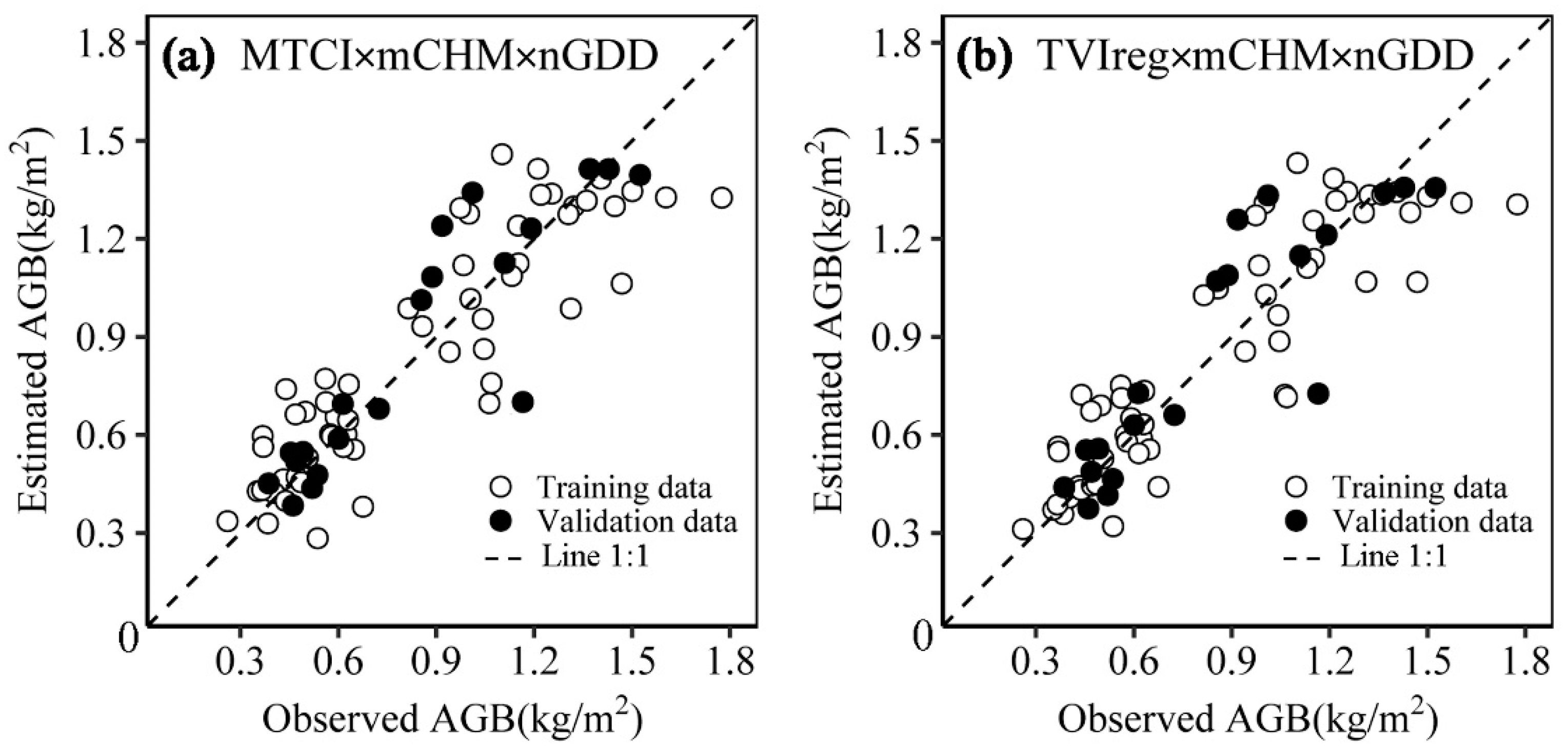
3.3.1. Performance Comparison of Data Fusion Using Pixel Level or Feature Level

This paper compared the wheat biomass estimation using both pixel-level and feature-level fusion with polynomial regression. The result was shown in Table 5.
It can be seen that the proposed metric using pixel-level fusion improved the estimation accuracy of wheat biomass. Both RMSE and nRMSE slightly decreased, while R2 slightly increased. These improvements indicated that the pixel-level fusion approach led to more accurate predictions of wheat biomass compared to the feature-level fusion approach, demonstrating the advantages of the pixel-wise accumulation method in maintaining the characteristics of canopy spatial variation [13]. Overall, the results suggested that pixel-level fusion using the proposed SM-CSRM was a promising approach for enhancing the accuracy of wheat biomass retrieval.

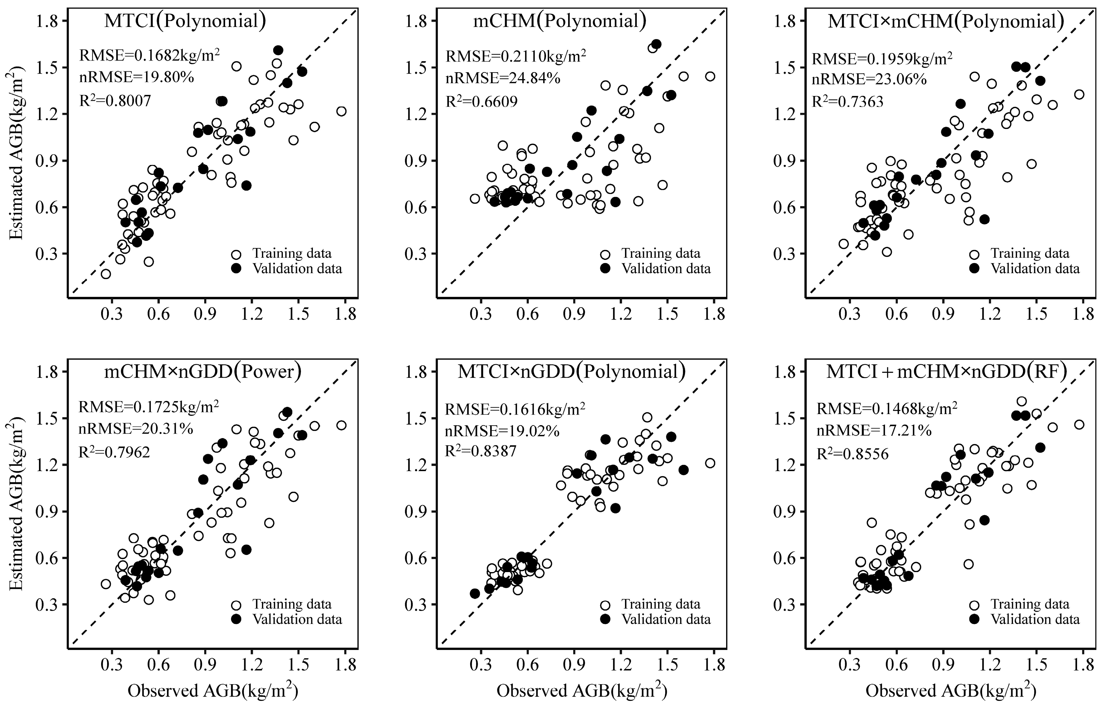
3.3.2. Statistical Modelling of Wheat AGB
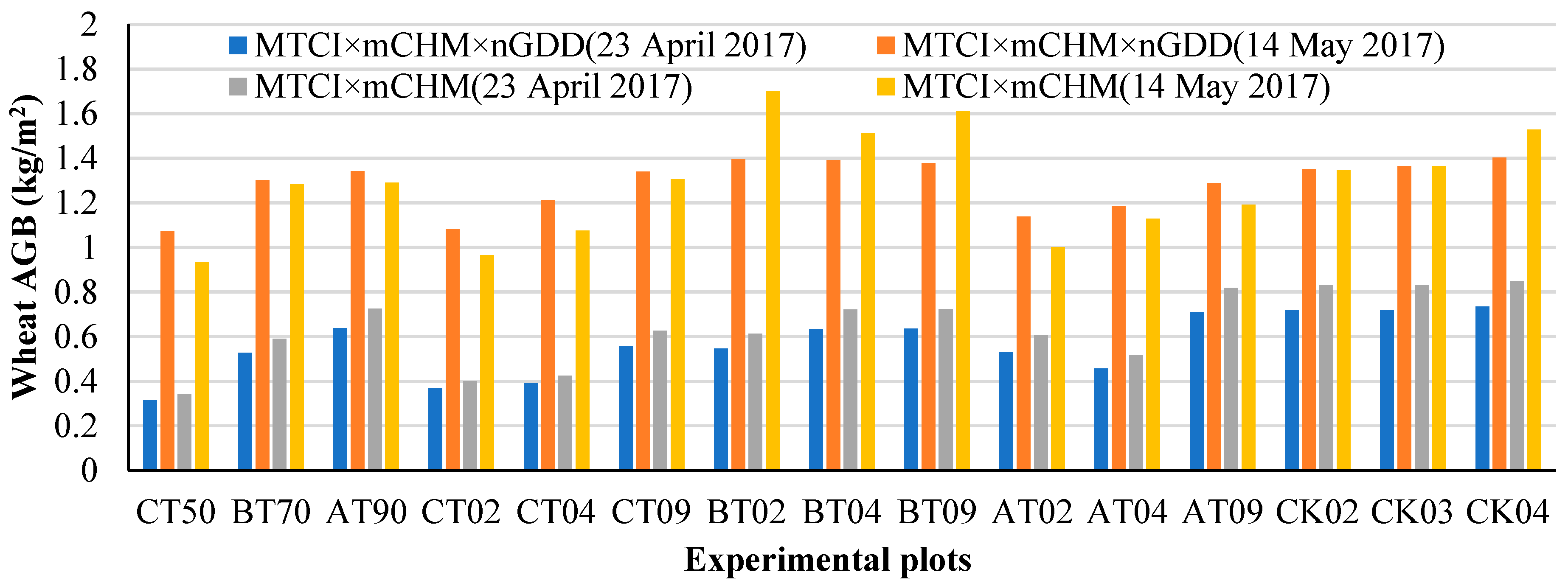
Statistical modelling of wheat AGB was estimated using polynomial regression for modelling and LOOCV for validation. The accuracy was evaluated using R2, RMSE and nRMSE. It can be seen from Table 6 that the best results were obtained for the metric of TVIreg × mCHM × nGDD (RMSE = 0.1782 kg/m2) in the training dataset and MTCI × mCHM × nGDD (RMSE = 0.1667 kg/m2) in the validating dataset, respectively.
Figure 6 showed the scatter plot representing the wheat biomass estimation results. The plot exhibited that the wheat estimation achieved good accuracy overall, but it also revealed a tendency to underestimate when dealing with higher quantities of biomass (>1.4~1.5 kg/m2). Similar studies have reported this phenomenon in the estimation of crop biomass [13]. Finally, the metric of MTCI × mCHM × nGDD was determined to estimate wheat AGB using polynomial regression.

3.3.3. AGB Mapping

AGB mapping was implemented by applying the estimated model to a raster format. This study conducted median filtering with a sliding window of size 3 × 3 to eliminate the potential outliers at local pixels. The final mapping results can be seen in Figure 7.

4. Discussion

4.1. Advantages of VIs Combining with CHM and GDD

The improvement ability of the proposed metrics with multi-feature fusion (SM-CSRM) is further analyzed by comparing the accuracy of different models for wheat biomass estimation. Specifically, the metrics of MTCI, mCHM, mCHM × nGDD, MTCI × mCHM, and MTCI × mCHM × nGDD were selected as the independent input variables for wheat biomass prediction. Table 7 shows the accuracy of the results of different models in order to demonstrate the performance of individual metrics and their combinations in efforts to forecast wheat biomass.
In Table 7, it can be seen that the estimation accuracy achieved using only the variable of structure information (mCHM) was significantly lower than that obtained in this study using only spectral input (MTCI). The use of mCHM derived from UAS multispectral images showed limited effectiveness in improving the wheat biomass prediction, and its accuracy even decreased when combining mCHM with MTCI. The meteorological factor nGDD contributed to enhance the estimation accuracy, and the accuracy predicted by mCHM × nGDD was slightly improved. However, the most optimal estimation was obtained by using the proposed metric (MTCI × mCHM × nGDD) with polynomial regression (R2 = 0.8069, RMSE = 0.1667 kg/m2), which enhanced the nRMSE by 3.44% with a multispectral image of 53 mm spatial resolution. In contrast, the estimated precision was slightly lower than that seen in similar literature for the prediction of wheat or soybean biomass. Wheat biomass was estimated, using only two spectral VIs with an nRMSE of 22.63% or only four image textures with an nRMSE of 21.24%, via multiple stepwise regression and using UAS optical images with an 11 mm ground sampling distance [18]. Similarly, soybean AGB was forecasted using a VI-weighted canopy volume model via linear regression and the use of 6 mm-resolution UAS RGB images, achieving an nRMSE of 16.3%. In summary, the proposed SM-CSRM metric, combining MTCI, mCHM, and nGDD, showed promising accuracy improvements in wheat biomass retrieval, although they were slightly lower than those obtained in some previous studies using different methodologies and higher-resolution imagery.
Figure 8 illustrated that the wheat biomass could be predicted with different levels of accuracy using spectral features (MTCI), structural features (mCHM) and meteorological factors (nGDD). In this study, the vegetation index involving the red-edge spectral band provided a good precision. However, a limitation of using only spectral indices was that they captured only one-dimensional information about the crop canopy, which tended to be saturation effects as biomass increased. Canopy structure traits can encompass both vertical and horizontal information, especially for UAS observations with a very high resolution. Notably, UAS multispectral imagery was demonstrated to obtain an accepted canopy height, although it exhibited somewhat lower precision compared to methods employing airborne optical or LiDAR sensors [26]. However, it even underestimated most of the samples with wheat biomass on the former observed date, and this was improved after pixel-level fusion with MTCI or nGDD.
The meteorological factor (nGDD) could improve the performance of UAS-based biomass estimation in the local scale after combination with canopy characteristics [20], such as spectral features (MTCI) and structural features (mCHM), or when used with combined spectral–structural features (MTCI × mCHM). These findings were in agreement with previous studies [13]. The improvement could be explained by the close relationship between crop biomass and climatic indicators, like GDD, and many climatic factors played a role in the physical models of crop parameters forecasting [30]. When considering the fusion of double variables, MTCI × nGDD displayed a higher RMSE than the other combination, but it was important to note that this combination presented two obvious clusters for two observed dates. This suggested that MTCI × nGDD might not be the best model for final AGB mapping with multiple observed dates.
Additionally, six figures of above-mentioned AGB modelling and mapping were attached in the Appendix A (see Figure A1, Figure A2, Figure A3, Figure A4, Figure A5 and Figure A6). Spatial variability was determined from the six results of biomass mapping. Particularly, spatial difference decreased after the combination of the input variable with nGDD, for instance MTCI versus MTCI× nGDD, mCHM versus mCHM × nGDD and MTCI × mCHM versus MTCI × mCHM × nGDD, especially for AGB mapping using MTCI × nGDD.

4.2. The Response of Estimated Crop Biomass to Typical Soil Profiles in Reclaimed Cropland

The crop response to the reclaimed soil environment was examined using the estimated AGB, as depicted in Figure 9. The figure displayed seven typical soil profiles that were chosen by considering the complexity of the reclamation activities, including three individual experimental plots (CT50, BT70, AT90) and three treatments (T02, T04, T09) with three duplicates in different cropland strips, as well as a control treatment (CK) with three duplicates. The mean AGB value of all pixels within each plot was employed by the statistical range inward 1 m distance from the plot boundary. Two sets of statistical AGB mapping were compared across the seven soil profiles in the figure. It was found that the proposed SM-CSRM showed a more stable and reliable prediction compared to structurally weighted canopy spectral response metric (S-CSRM) within the same treatment across different cropland lines, such as T02, T04 and T09 distributed in Line A, B and C, as well as CK treatment in Line CK. Notably, three samples (BT02, BT04, BT09) obtained apparently higher biomass than the control samples (CK02, CK03, CK04) for S-CSRM estimation on 14 May 2017. This discrepancy further confirmed the better performance of the proposed SM-CSRM over S-CSRM. The control treatment (CK) produced the highest wheat biomass with relative stability status across the two development stages, as seen in particular on 23 April 2017. This observation suggested that the plants in the control treatment were less stressed by the soil environment, resulting in better growth and biomass production.
The performance of typical soil profiles was reflected in the wheat biomass. Firstly, soil profiles consisting of a single layer of Yellow River sediments (CT50, BT70, AT90) showed higher predicted AGB as the effective soil thickness (comprising topsoil and subsoil) increased by 50 cm, 70 cm and 90 cm on the two surveying dates. Additionally, BT70 and CT90 displayed the relative difference of wheat biomass on 23 April 2017, but this variation became less apparent on 14 May 2017 after the rainfall and field management. This highlighted the importance of the thickness of topsoil and subsoil, particularly during the early period of crop development. This result aligned with the soil thickness (70 cm) recommended by the local regulation of cropland consolidation. Secondly, for the soil profiles composed of multilayer Yellow River sediments (T02, T04, T09), the estimated biomass displayed a positive correlation with soil layer thickness. Specifically, thicker soil layers were associated with higher crop biomass for three treatments (T02, T04 and T09) across different cropland strips (Line A, B and C). Similar changing trends were observed within the same cropland strip, while variations existed among the three cropland lines. Besides the minor disturbance by the local farmer in the plot of AT04 before 23 April 2017, the lowest and highest averaging biomass were consistently observed in soil profiles of T02 and T09 across the three cropland lines for both two observation dates, respectively. These findings underscored that soil thickness was significant during cropland reclamation using multilayer Yellow River sediments. Furthermore, according to the field investigation, the different crop phenotypes in three cropland lines were related to the actual thickness of topsoil and subsoil after soil reconstruction. The soil thickness of Line B is universally thicker than that of the other two lines. These findings were in accordance with the previous research [31].

4.3. The Implications and Applicability of the Proposed SM-CSRM

The metric (SM-CSRM) proposed in this paper has an exact physical meaning. Firstly, the coefficient of p and q were determined by examining the correlation between the wheat biomass and each selected VI variable. CHM and GDD have positive correlations with wheat biomass, leading to concurrent positive values for p and q. However, different VIs might show positive or negative correlation with wheat biomass at different growing stages or their combinations. Secondly, the value range of CHM, GDD and VIs was taken into account. The theoretical minimum value of CHM is zero, indicating bare ground without vegetation. The maximum value of CHM varies based on factors like crop variety, field management and growth environment. Similarly, the minimum value of GDD is zero when crop seeds are ready to grow just after sowing. The maximum value of GDD depends on crop varieties and meteorological conditions. The value range of VIs differs, and certain scenarios, such as when a VI pixel value is zero and its exponential coefficient is negative, could lead to infinite values, which in turn could pose challenges for programing computation. However, VIs have long been recognized as crucial predictors for AGB estimation. Therefore, this paper introduced the vegetation-masked CHM and normalized GDD, incorporating their corresponding exponential coefficients as weights for the VI. In the future, more structural and climatic factors should be explored to improve the estimated accuracy of wheat biomass.
VIs serve as indicators of the spectral response exhibited by a crop canopy and they correlate highly with the growth status of crops at different development stages. Different VIs show varying degrees of correlation with the growth parameters of crops. In this study, 13 VIs containing red-edge bands showed relatively higher correlation with AGB compared to VIs without red-edge bands. VIs containing red-edge bands have been proved to be strongly correlated with plant parameters like SPAD [22] and LAI [32]. Specifically, NDVI and SR were negatively correlated with the wheat AGB during two observed dates, with correlations of −0.4982 and −0.588, respectively. However, NDVIreg and SRreg showed positive correlations with AGB for 0.8222 and 0.8253, respectively, because the wheat had a good spectral response (higher values of NDVI) in vegetative growth at the jointing stage (23 April 2017) and a poor spectral response (lower values of NDVI) in reproductive growth at flowering stage (14 May 2017). It also indicated that data acquisition should properly select the crop growth stage.
CHM is a commonly utilized structure data type that is often employed to assess the characteristics of vegetation canopies. However, its performance in data fusion with VI demonstrated limitations in this study, which can potentially lead to relatively lower prediction accuracy when using UAS-based multispectral data. It was worth considering that UAS-based RGB or LiDAR data can offer alternative approaches with the capacity to improve the estimation accuracy of plant height.
Meteorological factors required gradual changes in spatial distribution and continuous temporal evolution. GDD is an indicator of accumulated effective temperature, which aligns well with the above-mentioned requirements. The suitability of GDD relates to its ability to reflect the cumulative impact of temperature on crop growth over time, which makes it an ideal metric for use in this kind of exercise. In contrast, precipitation is unbalanced in its spatial and temporal distribution, which is not suitable for UAS-based biomass estimation at a fine scale. Besides, the total evapotranspiration is usually calculated using the Penman equation, which needs multiple climate parameters, but many meteorological stations provide poor-quality data [33]. From the perspective of data acquisition, the density of meteorological stations can basically support the monitoring needs because the average distance of neighboring national-level meteorological stations is around 10~20 km in the central and eastern parts of China. There is denser coverage for regional-level stations. Moreover, daily observation elements only encompass five items: maximum temperature, minimum temperature, precipitation, wind speed and wind direction. Notably, precipitation records may be absent during the winter period.
Crops with similar row crops and canopy traits might be suitable for utilizing the proposed framework for above-ground biomass estimation, and the specific field can be applied in the effect evaluation of reclaimed cropland or in the potential utilization of crop breeding for precision agriculture.

4.4. Limitations and Future Work of the Proposed SM-CSRM

This study explained the potential of combining UAS multispectral data with temperature information to estimate crop biomass through pixel-level data fusion, integrating canopy spectral features with plant structure and environmental factor of temperature. As such, the limitations should be stated to assist further efforts to improve the performance of this approach.
Single factors of data fusion in crop biomass estimation have limitations in terms of data acquisition and analysis. Firstly, the optimal spectral response traits should be further explored for either a single date or combined dates. In this paper, NDVI and SR displayed a negative correlation with measured AGB in two combined observations, and they achieved unsatisfactory results when combined with canopy height. This was because many VIs increased to the highest values as crops grew, and then decreased over time. This phenomenon can be also illustrated by a previous study of crop biomass prediction using two development periods [29]. Therefore, more crop growth stages should be observed in order to identify the optimal spectral response (VIs) at various growing periods, and each surveying stage should be examined to perform biomass estimation. Secondly, the accuracy of canopy structure information might limit the retrieved performance of proposed SM-CSRM. Several UAS-derived approaches could be compared and employed to extract the canopy structure, such as optical or LiDAR sensors [26]. CHM with the higher accuracy should be surveyed more extensively [13], and other plant structural traits should also be considered, in order to enhance biomass retrieval [15]. Thirdly, meteorological indicators showed a good relationship with crop biomass, but only GDD was utilized as a point value for a specific date. The spatial variation of GDD or other climatic factors was considerable for the larger scale, which could potentially lead to more accurate estimates.
In future, the influencing mechanism behind the combination of spectral, structural features and meteorological factors should be further explored to perform wheat biomass predictions. Notably, wheat biomass revealed a strong correlation (0.8816) with MTCI and a weak correlation (0.6405) with mCHM derived from UAS multispectral data, but soybean biomass showed an comparable correlation (0.889) with CHmean and a lower correlation (0.544) with the selected VI (green–red ratio index, GRRI) [13], but their combinations exhibited varying abilities for biomass forecasting. Thus, these combinations should be examined under different conditions of crop cultivation and field management to improve the robustness of the proposed SM-CSRM and achieve more accurate estimations for the assessment of reclaimed cropland or precision agriculture. Besides, more observed dates and their combinations should be further explored to provide guidelines for UAS data collection about different cultivated crop types. The scale effect of UAS observations with different flight height should also be investigated for each individual factor and combined metrics, a practice which helps to identify the optimal flight altitude. In addition, this study was only verified using winter wheat in a relatively small reclaimed experimental site of 1200 m2. Consequently, the robustness of the proposed metric should be further tested under more complex environment and field management situations relevant to reclaimed cropland or precision agriculture, such as diverse sites, various crop varieties and cultivation density, or more stage combinations of different crop development phases.
Besides, the reclaimed cropland was required to be restored to the original level of crop production by national regulations, requiring a recovery period of 3~5 years. The proposed SM-CSRM considered both the potential height of crop canopies and interannual variations using normalized GDD. As a result, it has the potential to significantly contribute to the interannual evaluation of reclaimed effects, but it should also be tested across a broader spectrum of reclaimed cropland with different crop densities or growing stages after the completion of reclamation activities. By accumulating data over more consecutive years, the proposed SM-CSRM can be further refined, validated and improved, thereby bolstering its utility in not only crop biomass forecasting but also for comprehensive assessments of reclaimed cropland.

5. Conclusions

This paper reported an improved metric, termed the structurally–meteorologically weighted canopy spectral response metric (SM-CSRM), for the accurate estimation of wheat AGB using UAS-based multispectral images. This novel metric was proposed via pixel-level data fusion combining the canopy spectral response (VI), structural information (vegetation-masked CHM) and meteorological factors (normalized GDD) as an independent input variable. The best metric was identified via qualitative analysis using Pearson correlation and quantitative analysis using the simple function fitting. Subsequently, an AGB estimation model was built using the optimal simple regression method and LOOCV. The results indicated that the proposed metrics (SM-CSRM) showed a nonlinear relationship with wheat AGB when integrating mCHM, nGDD and a highly correlated VI. The metric (MTCI × mCHM × nGDD) achieved the highest level of accuracy in biomass estimation using polynomial regression (R2 = 0.8069, RMSE = 0.1667 kg/m2, nRMSE = 19.62%), exhibiting improvement on predictions solely made using MTCI or mCHM as variables. Additionally, VI incorporating the red-edge band presented strong correlation with wheat biomass, such MTCI and TVIreg. GDD was demonstrated to be a greatly useful indicator for AGB estimation. The performance of pixel-level data fusion demonstrated advantages over feature-level fusion. This study offers contributions by facilitating the accurate estimation of wheat AGB and efficient assessment of reclaimed cropland or precision agriculture. These advancements hold potential benefits for enhanced crop monitoring and field management practices.

Author Contributions

Conceptualization, all authors; methodology and formal analysis, J.Z. and W.X.; software, J.Z.; validation, J.Z.; investigation, J.Z. and W.X.; data curation, J.Z.; writing—original draft preparation, J.Z.; writing—review and editing, Y.Z., Z.H. and W.X.; funding acquisition, Y.Z., W.X. and J.Z. All authors have read and agreed to the published version of the manuscript.

Funding

This research was supported by the National Natural Science Foundation of China under Grant [number 42071250], Key Laboratory of Digital Mapping and Land Information Application, Ministry of Natural Resources under Grant [number ZRZYBWD202204].

Institutional Review Board Statement

Not applicable.

Data Availability Statement

The authors do not have permission to share data.

Acknowledgments

Thanks to Shuo Zhang, Yuzhu Zou and Shuaishuai Tian for the field data collection.

Conflicts of Interest

The authors declare no conflict of interest.

Appendix A

Table A1. Name and equation list of selected vegetation indices.
NO.VI NameEquation
1Simple ratio vegetation index, SR S R = ρ N I R ρ R
2Modified ratio vegetation index, MSR M S R = ρ N I R ρ R 1 ρ N I R ρ R + 1
3Normalized difference vegetation index, NDVI N D V I = ρ N I R ρ R ρ N I R + ρ R
4Renormalized difference vegetation index, RDVI R D V I = ρ N I R ρ R ρ N I R + ρ R
5Enhanced vegetation index, EVI E V I = ρ N I R ρ R 1 + ρ N I R + 2.4 ρ R
6Difference vegetation index, DVI D V I = ρ N I R ρ R
7Triangular vegetation index, TVI T V I = 60 ( ρ N I R ρ G ) 100 ( ρ R ρ G )
8Optimized soil adjustment vegetation index, OSAVI O S A V I = ρ N I R ρ R ρ N I R + ρ R + 0.16
9Modified soil adjustment vegetation index, MSAVI M S A V I = 2 ρ N I R + 1 ( ρ N I R + 1 ) 2 8 ( ρ N I R ρ R ) 2
10Modified Nonlinear vegetation index, MNLI M N L I = 1.5 ( ρ N I R 2 ρ G ) ρ N I R 2 + ρ R + 0.5
11MERIS Terrestrial Chlorophyll Index, MTCI M T C I = ρ N I R ρ Re g ρ Re g ρ R
12Soil adjustment vegetation index, SAVI S A V I = ( 1 + L ) ρ N I R ρ R ρ N I R + ρ R + 1 ,   L = 0 . 5
13Chlorophyll vegetation index—green, CIgreen C I g r e e n = ρ N I R ρ R 1
14Simple ratio vegetation index—red edge, SRreg S R r e g = ρ N I R ρ Re g
15Modified ratio vegetation index—red edge, MSRreg M S R r e g = ρ N I R ρ Re g 1 ρ N I R ρ Re g + 1
16Normalized difference vegetation index—red edge, NDVIreg N D V I r e g = ρ N I R ρ Re g ρ N I R + ρ Re g
17Renormalized difference vegetation index—red edge, RDVIreg R D V I r e g = ρ N I R ρ Re g ρ N I R + ρ Re g
18Enhanced vegetation index—red edge, EVIreg E V I r e g = ρ N I R ρ Re g 1 + ρ N I R + 2.4 ρ Re g
19Difference vegetation index—red edge, DVIreg D V I r e g = ρ N I R ρ Re g
20Triangular vegetation index—red edge, TVIreg T V I r e g = 60 ( ρ N I R ρ G ) 100 ( ρ Re g ρ G )
21Optimized soil adjustment vegetation index—red edge, OSAVIreg O S A V I r e g = ρ N I R ρ Re g ρ N I R + ρ Re g + 0.16
22Modified soil adjustment vegetation index, MSAVIreg M S A V I r e g = 2 ρ N I R + 1 ( ρ N I R + 1 ) 2 8 ( ρ N I R ρ R e g ) 2
23Modified Nonlinear vegetation index—red edge, MNLIreg M N L I r e g = 1.5 ( ρ N I R 2 ρ G ) ρ N I R 2 + ρ R e g + 0.5
24Soil adjustment vegetation index, SAVIreg S A V I r e g = ( 1 + L ) ρ N I R ρ Re g ρ N I R + ρ Re g + 1 ,   L = 0 . 5
25Chlorophyll vegetation index—red edge, CIreg C I r e g = ρ N I R ρ R e g 1
Note: ρ G , ρ R , ρ Re g and ρ N I R are the band reflectance of green, red, red-edge and near-infrared, respectively.
Figure A1. Wheat AGB prediction using MTCI as the input and polynomial regression.
Agriculture 13 01621 g0a1
Figure A2. Wheat AGB prediction using MTCI × nGDD as the input and polynomial regression.
Agriculture 13 01621 g0a2
Figure A3. Wheat AGB prediction using mCHM as the input and polynomial regression.
Agriculture 13 01621 g0a3
Figure A4. Wheat AGB prediction using mCHM × nGDD as the input and power regression.
Agriculture 13 01621 g0a4
Figure A5. Wheat AGB prediction using MTCI × mCHM as the input and polynomial regression.
Agriculture 13 01621 g0a5
Figure A6. Wheat AGB prediction using MTCI and mCHM × nGDD as the inputs and Random Forest regression.
Agriculture 13 01621 g0a6

References

  1. Avolio, M.L.; Hoffman, A.M.; Smith, M.D. Linking gene regulation, physiology, and plant biomass allocation in Andropogon gerardii in response to drought. Plant Ecol. 2018, 219, 1–15. [Google Scholar] [CrossRef]
  2. Luis Araus, J.; Cairns, J.E. Field high-throughput phenotyping: The new crop breeding frontier. Trends Plant Sci. 2014, 19, 52–61. [Google Scholar] [CrossRef]
  3. Ren, H.; Xiao, W.; Zhao, Y.; Hu, Z. Land damage assessment using maize aboveground biomass estimated from unmanned aerial vehicle in high groundwater level regions affected by underground coal mining. Environ. Sci. Pollut. Res. 2020, 27, 21666–21679. [Google Scholar] [CrossRef]
  4. Zhao, Y.; Zheng, W.; Xiao, W.; Zhang, S.; Lv, X.; Zhang, J. Rapid monitoring of reclaimed farmland effects in coal mining subsidence area using a multi-spectral UAV platform. Environ. Monit. Assess. 2020, 192, 474. [Google Scholar] [CrossRef] [PubMed]
  5. Hensgen, F.; Bühle, L.; Wachendorf, M. The effect of harvest, mulching and low-dose fertilization of liquid digestate on above ground biomass yield and diversity of lower mountain semi-natural grasslands. Agric. Ecosyst. Environ. 2016, 216, 283–292. [Google Scholar] [CrossRef]
  6. Bhandari, M.; Ibrahim, A.M.H.; Xue, Q.; Jung, J.; Chang, A.; Rudd, J.C.; Maeda, M.; Rajan, N.; Neely, H.; Landivar, J. Assessing winter wheat foliage disease severity using aerial imagery acquired from small Unmanned Aerial Vehicle (UAV). Comput. Electron. Agric. 2020, 176, 105665. [Google Scholar] [CrossRef]
  7. Vergara-Diaz, O.; Zaman-Allah, M.A.; Masuka, B.; Hornero, A.; Zarco-Tejada, P.; Prasanna, B.M.; Cairns, J.E.; Araus, J.L. A novel Remote Sensing approach for prediction of maize yield under different conditions of nitrogen fertilization. Front. Plant Sci. 2016, 7, 666. [Google Scholar] [CrossRef]
  8. Breiman, A.; Graur, D. Wheat evolution. Isr. J. Plant Sci. 1995, 43, 85–98. [Google Scholar] [CrossRef]
  9. Marshall, M.; Thenkabail, P. Advantage of hyperspectral EO-1 Hyperion over multispectral IKONOS, GeoEye-1, WorldView-2, Landsat ETM plus, and MODIS vegetation indices in crop biomass estimation. ISPRS J. Photogramm. Remote Sens. 2015, 108, 205–218. [Google Scholar] [CrossRef]
  10. Poley, L.G.; McDermid, G.J. A Systematic Review of the Factors Influencing the Estimation of Vegetation Aboveground Biomass Using Unmanned Aerial Systems. Remote Sens. 2020, 12, 1052. [Google Scholar] [CrossRef]
  11. Li, W.; Niu, Z.; Huang, N.; Wang, C.; Gao, S.; Wu, C. Airborne LiDAR technique for estimating biomass components of maize A case study in Zhangye City, Northwest China. Ecol. Indic. 2015, 57, 486–496. [Google Scholar] [CrossRef]
  12. Yue, J.; Yang, G.; Li, C.; Li, Z.; Wang, Y.; Feng, H.; Xu, B. Estimation of Winter Wheat Above-Ground Biomass Using Unmanned Aerial Vehicle-Based Snapshot Hyperspectral Sensor and Crop Height Improved Models. Remote Sens. 2017, 9, 708. [Google Scholar] [CrossRef]
  13. Maimaitijiang, M.; Sagan, V.; Sidike, P.; Maimaitiyiming, M.; Hartling, S.; Peterson, K.T.; Maw, M.J.W.; Shakoor, N.; Mockler, T.; Fritschi, F.B. Vegetation Index Weighted Canopy Volume Model (CVMVI) for soybean biomass estimation from Unmanned Aerial System-based RGB imagery. ISPRS J. Photogramm. Remote Sens. 2019, 151, 27–41. [Google Scholar] [CrossRef]
  14. Hunt, E.R., Jr.; Daughtry, C.S. What good are unmanned aircraft systems for agricultural remote sensing and precision agriculture? Int. J. Remote Sens. 2018, 39, 5345–5376. [Google Scholar] [CrossRef]
  15. Jiang, Q.; Fang, S.; Peng, Y.; Gong, Y.; Zhu, R.; Wu, X.; Ma, Y.; Duan, B.; Liu, J. UAV-based biomass estimation for rice-combining spectral, TIN-based structural and meteorological features. Remote Sens. 2019, 11, 890. [Google Scholar] [CrossRef]
  16. Li, B.; Xu, X.; Zhang, L.; Han, J.; Bian, C.; Li, G.; Liu, J.; Jin, L. Above-ground biomass estimation yield prediction in potato by using UAV-based, R.G.B.; hyperspectral imaging. ISPRS J. Photogramm. Remote Sens. 2020, 162, 161–172. [Google Scholar] [CrossRef]
  17. Greaves, H.E.; Vierling, L.A.; Eitel, J.U.; Boelman, N.T.; Magney, T.S.; Prager, C.M.; Griffin, K.L. Estimating aboveground biomass leaf area of low-stature Arctic shrubs with terrestrial LiDAR. Remote Sens. Environ. 2015, 164, 26–35. [Google Scholar] [CrossRef]
  18. Yue, J.; Yang, G.; Tian, Q.; Feng, H.; Xu, K.; Zhou, C. Estimate of winter-wheat above-ground biomass based on UAV ultrahigh-ground-resolution image textures vegetation indices. ISPRS J. Photogramm. Remote Sens. 2019, 150, 226–244. [Google Scholar] [CrossRef]
  19. Zhang, L.; Zhang, Z.; Luo, Y.; Cao, J.; Xie, R.; Li, S. Integrating satellite-derived climatic and vegetation indices to predict smallholder maize yield using deep learning. Agric. Forest Meteorol. 2021, 311, 108666. [Google Scholar] [CrossRef]
  20. Ballesteros, R.; Ortega, J.F.; Hernandez, D.; Del Campo, A.; Moreno, M.A. Combined use of agro-climatic very high-resolution remote sensing information for crop monitoring. Int. J. Appl. Earth Obs. Geoinf. 2018, 72, 66–75. [Google Scholar] [CrossRef]
  21. Prabhakara, K.; Hively, W.D.; McCarty, G.W. Evaluating the relationship between biomass, percent groundcover and remote sensing indices across six winter cover crop fields in Maryland, United States. Int. J. Appl. Earth Obs. Geoinf. 2015, 39, 88–102. [Google Scholar] [CrossRef]
  22. Deng, L.; Mao, Z.; Li, X.; Hu, Z.; Duan, F.; Yan, Y. UAV-based multispectral remote sensing for precision agriculture: A comparison between different cameras. ISPRS J. Photogramm. Remote Sens. 2018, 146, 124–136. [Google Scholar] [CrossRef]
  23. Wang, Y.; Hu, C.; Dong, W.; Li, X.; Zhang, Y.; Qin, S.; Oenema, O. Carbon budget of a winter-wheat and summer-maize rotation cropland in the north china plain. Agric. Ecosyst. Environ. 2015, 206, 33–45. [Google Scholar] [CrossRef]
  24. Yue, J.; Feng, H.; Li, Z.; Zhou, C.; Xu, K. Mapping winter-wheat biomass grain yield based on a crop model UAV remote sensing. Int. J. Remote Sens. 2020, 42, 1577–1601. [Google Scholar] [CrossRef]
  25. Zhao, P.; Lu, D.; Wang, G.; Wu, C.; Huang, Y.; Yu, S. Examining spectral reflectance saturation in landsat imagery and corresponding solutions to improve forest aboveground biomass estimation. Remote Sens. 2016, 8, 469. [Google Scholar] [CrossRef]
  26. Zhang, J.; Hu, Z.; Zhao, Y.; Xiao, W.; Yang, K.; Chen, J. Estimating canopy surface height of wheat corn crops in reclaimed cropland using multispectral images from a small unmanned aircraft system. J. Appl. Remote Sens. 2021, 15, 034506. [Google Scholar] [CrossRef]
  27. Rodriguez-Galiano, V.F.; Ghimire, B.; Rogan, J.; Chica-Olmo, M.; Rigol-Sanchez, J.P. An assessment of the effectiveness of a random forest classifier for land-cover classification. ISPRS J. Photogramm. Remote Sens. 2012, 67, 93–104. [Google Scholar] [CrossRef]
  28. Zhao, B.; Zhang, Q.; Wang, W. Research on Biological Zero and Accumulated Temperature of 11 Kinds of Plant Seeds Germination in the North China Plain. Chin. Wild Plant Resour. 2014, 32, 20–23. [Google Scholar]
  29. Wan, L.; Zhang, J.; Dong, X.; Du, X.; Zhu, J.; Sun, D.; Liu, Y.; He, Y.; Cen, H. Unmanned aerial vehicle-based field phenotyping of crop biomass using growth traits retrieved from PROSAIL model. Comput. Electron. Agric. 2021, 187, 106304. [Google Scholar] [CrossRef]
  30. Li, J.; Wijewardane, N.K.; Ge, Y.; Shi, Y. Improved chlorophyll and water content estimations at leaf level with a hybrid radiative transfer and machine learning model. Comput. Electron. Agric. 2023, 206, 107669. [Google Scholar] [CrossRef]
  31. Hu, Z.; Shao, F.; McSweeney, K. Reclaiming subsided land with Yellow River sediments: Evaluation of soil-sediment columns. Geoderma 2017, 307, 210–219. [Google Scholar] [CrossRef]
  32. Dong, T.; Liu, J.; Shang, J.; Qian, B.; Ma, B.; Kovacs, J.M.; Walters, D.; Jiao, X.; Geng, X.; Shi, Y. Assessment of red-edge vegetation indices for crop leaf area index estimation. Remote Sens. Environ. 2019, 222, 133–143. [Google Scholar] [CrossRef]
  33. Ballesteros, R.; Ortega, J.F.; Moreno, M.Á. FORETo: New software for reference evapotranspiration forecasting. J. Arid Environ. 2016, 124, 128–141. [Google Scholar] [CrossRef]
Figure 1. The location of the study area and its layout. (a) The location in China; (b) the location in the Shandong Province; (c) the layout of different soil-sediment profiles in the study area and the distribution of 38 samples.
Agriculture 13 01621 g001
Figure 2. The schematic diagram of profiles with different reclaimed thickness using local soil and Yellow River sediments.
Agriculture 13 01621 g002
Figure 3. The UAS platform (DJI Matrice 100) and the multispectral camera (Parrot Sequoia).
Agriculture 13 01621 g003
Figure 4. The workflow of wheat AGB estimation using the proposed metric combining the structural and meteorological data with the canopy spectral information.
Agriculture 13 01621 g004
Figure 5. Pearson correlation coefficient between AGB and VI, VI × mCHM, the proposed metric for wheat. Dashed line is the value of r m C H M (0.6405) between wheat AGB and mCHM in the two growth stages.
Agriculture 13 01621 g005
Figure 6. Scatter plots of observed and estimated wheat AGB using (a) MTCI × mCHM × nGDD and (b) TVIreg × mCHM × nGDD as an input variable.
Agriculture 13 01621 g006
Figure 7. Mapping of estimated wheat above-ground biomass: (a) 23 April 2017, (b) 14 May 2017.
Agriculture 13 01621 g007
Figure 8. The scatter plots for observed and estimated AGB using different inputs with the optimal regression.
Agriculture 13 01621 g008
Figure 9. Estimated wheat AGB in seven typical soil profiles.
Agriculture 13 01621 g009
Table 1. GDD results of crop-observed dates in the experimental site.
DateDays after Sowing (DAS)GDD (°C·d)nGDDNotes
5 October 2016112.30.0131sowing
23 April 20172013460.3699
14 May 2017222568.80.6080
8 June 2017247935.41harvest
Table 2. The popular simple fitting functions.
NO.Fitting FunctionFunction Equation
1Linear functionY = aX + b
2Polynomial functionY = aX2 + bX + c
3Power functionY = aXb
4Exponential functionY = ae (bX)
5Logarithmic functionY = alnX + b
Notes: Y is the dependent variable (crop biomass); X is the independent variable (the proposed SM-CSRM); a, b, and c are constant.
Table 3. Correlation coefficient between vegetation indexes and measured wheat AGB.
NO.VIsPearson Correlation (r)Spearman Rank-Order Correlation (rs)
1CIgreen0.3311 **0.3919 **
2CIreg0.8253 **0.8375 **
3DVI0.8396 **0.8344 **
4DVIreg0.8686 **0.8637 **
5EVI0.7981 **0.8147 **
6EVIreg0.8625 **0.8654 **
7MNLI0.8035 **0.816 **
8MNLIreg0.8636 **0.8641 **
9MSAVI0.8527 **0.8277 **
10MSAVIreg0.8589 **0.8396 **
11MSR−0.5764 **−0.5614 **
12MSRreg0.8248 **0.8367 **
13MTCI0.8816 **0.8884 **
14NDVI−0.4982 **−0.5426 **
15NDVIreg0.8222 **0.8358 **
16OSAVI0.5999 **0.6429 **
17OSAVIreg0.8482 **0.8516 **
18RDVI0.7622 **0.7834 **
19RDVIreg0.8611 **0.8647 **
20SAVI0.7863 **0.8053 **
21SAVIreg0.8609 **0.8646 **
22SR−0.588 **−0.5655 **
23SRreg0.8253 **0.8375 **
24TVI0.8338 **0.8323 **
25TVIreg0.8754 **0.881 **
Notes: ** represents the significant correlation at the 0.01 level; NS represents not significant.
Table 4. Five optimal univariate fitting results between wheat AGB and proposed SM-CSRM.
NO.Input VariableFitting TypeOptimal Fitting ResultR2RMSE (kg/m2)
1DVIreg × mCHM × nGDDLineary = 9.764x + 0.31150.78310.1804
Polynomialy = −54.67x2 + 16.77x + 0.15720.79870.1751
Powery = 5.167x0.60550.79560.1752
Exponentialy = 0.4594exp(10.08x)0.74250.1966
Logarithmicy = 0.4936ln(x) + 2.3890.78030.1816
2EVIreg × mCHM × nGDDLineary = 18.67x + 0.28250.78130.1812
Polynomialy = −185x2 + 31.7x + 0.11810.79530.1765
Powery = 8.446x0.6450.78900.1768
Exponentialy = 0.447exp(19.22x)0.74110.1972
Logarithmicy = 0.5303ln(x) + 2.8050.77740.1828
3MSAVI × mCHM × nGDDLineary = 2.668x + 0.21410.79900.1737
Polynomialy = −1.973x2 + 3.707x + 0.11090.80260.1733
Powery = 2.487x0.72810.80180.1725
Exponentialy = 0.4017exp(2.868x)0.77190.1850
Logarithmicy = 0.5883ln(x) + 1.7790.77910.1821
4MTCI × mCHM × nGDDLineary = 1.584x + 0.29220.78530.1795
Polynomialy = −1.541x2 + 2.865x + 0.10260.80580.1719
Powery = 1.725x0.63510.79970.1734
Exponentialy = 0.4586exp(1.593x)0.73710.1987
Logarithmicy = 0.5309ln(x) + 1.5080.79050.1774
5TVIreg × mCHM × nGDDLineary = 0.2435x + 0.41790.77770.1827
Polynomialy = −0.0449x2 + 0.4419x + 0.29340.80900.1705
Powery = 0.7112x0.46150.80350.1718
Exponentialy = 0.5258exp(0.2408x)0.72180.2044
Logarithmicy = 0.351ln(x) + 0.78360.76370.1883
Table 5. Accuracy validation of wheat AGB estimation using pixel-level or feature-level data fusion.
Way of Data FusionIndependent VariableR2RMSE (kg/m2)nRMSE (%)
Pixel-level(MTCI × mCHM × nGDD)_mean0.80690.166719.62
Feature-levelMTCI_mean × mCHM_mean × nGDD0.80460.167419.71
Pixel-level(TVIreg × mCHM × nGDD)_mean0.78650.172420.29
Feature-levelTVIreg_mean × mCHM_mean × nGDD0.77880.174820.58
Table 6. Modelling accuracy of polynomial regression for wheat AGB estimation.
Input VariablesDatasetR2RMSE (kg/m2)nRMSE (%)
MTCI × mCHM × nGDDTraining0.78400.182321.46
TVIreg × mCHM × nGDDTraining0.79350.178220.98
MTCI × mCHM × nGDDValidation0.80690.166719.62
TVIreg × mCHM × nGDDValidation0.78650.172420.29
Table 7. Validation statistics of wheat AGB estimation using different univariate regression.
Independent VariableRegression MethodR2RMSE (kg/m2)nRMSE (%)
MTCIPolynomial0.80070.168219.80
mCHMPolynomial0.66090.211024.84
MTCI × mCHMPolynomial0.73630.195923.06
mCHM × nGDDPolynomial0.79450.175020.61
MTCI × mCHM × nGDDPolynomial0.80690.166719.62
Disclaimer/Publisher’s Note: The statements, opinions and data contained in all publications are solely those of the individual author(s) and contributor(s) and not of MDPI and/or the editor(s). MDPI and/or the editor(s) disclaim responsibility for any injury to people or property resulting from any ideas, methods, instructions or products referred to in the content.

