Extrapolation of Tractor Traction Resistance Load Spectrum and Compilation of Loading Spectrum Based on Optimal Threshold Selection Using a Genetic Algorithm

Abstract

To obtain the load spectrum of the traction resistance of the three-point suspension device under tractor-plowing conditions, a load spectrum extrapolation method based on a genetic algorithm optimal threshold selection is proposed. This article first uses a pin force sensor to measure the plowing resistance of the tractor’s three-point suspension device under plowing conditions and preprocesses the collected load signal. Next, a genetic algorithm is introduced to select the threshold based on the Peak Over Threshold (POT) extremum extrapolation model. The Generalized Pareto Distribution (GPD) fits the extreme load distribution that exceeds the threshold range, generating new extreme points that follow the GPD distribution to replace the extreme points in the original data, achieving the extrapolation of the load spectrum. Finally, the loading spectrum that can be achieved on the test bench is obtained based on the miner fatigue theory and accelerated life theory. The results show that the upper threshold of the time-domain load data obtained by the genetic algorithm is 10.975 kN, and the grey correlation degree is 0.7249. The optimal lower threshold is 8.5455 kN, the grey correlation degree is 0.7722, and the fitting effect of the GPD distribution is good. The plowing operation was divided into five stages: plowing tool insertion, acceleration operation, constant speed operation, deceleration operation, and plowing tool extraction. A traction resistance loading spectrum that can be achieved on the test bench was developed. The load spectrum extrapolation method based on the genetic algorithm optimal threshold selection can improve the accuracy of threshold selection and achieve the extrapolation and reconstruction of the load spectrum. After processing the extrapolated load spectrum, it can be transformed into a load spectrum that can be recognized by the test bench.

1. Introduction

During farming operations in the field, the load spectrum of a tractor is subjected to random loads due to the complex and variable environment. The load spectrum is a load time history that reflects the loading situation of the entire structure or key components [1], containing load information and the distribution law of the tractor under operating conditions [2]. By extrapolating and reconstructing the load spectrum, a full-life-cycle load spectrum can be obtained within a finite detection time of the load spectrum, thereby reducing time and testing costs. This is of great significance for predicting fatigue life and conducting reliability testing of various components of tractors [3]. The extrapolated load spectrum cannot directly guide relevant performance tests. To facilitate the loading of the test bench, it is necessary to convert the load spectrum into a constant stress spectrum, i.e., to compile the load spectrum.

In recent years, the application of load spectrum extrapolation in agricultural machinery has become increasingly widespread. Shao et al. established a load transfer model for tractor plowing operations and analyzed the load characteristics of the tractor transmission system for field plowing operations through rainfall basin extrapolation [4]. Roberto Tovo proposed a new method to evaluate the single Weibull distribution of the period generated by the rainflow count of random processes, which provides a basis for reliability analysis of fatigue behavior of actual components under service loads [5]. Wang et al. proposed a tractor power take-off (PTO) torque load spectrum extrapolation method based on FDR (False Discovery Rate) threshold automatic selection and optimized the time-domain extrapolation threshold selection method [6]. Yang et al. proposed a time-domain load extrapolation method based on the EMD-POT (Empirical mode decomposition-peaks over threshold) model to address the two issues of insufficient adaptability of traditional POT extrapolation methods to non-stationary loads and the lack of discussion on extrapolation reconstruction. The stability of the mean and standard deviation of this extrapolation reconstruction method has been improved by 28.5% and 31.2%, respectively. Compared with the random reconstruction method, the damage consistency has been improved by 9.4% [7]. He et al. address the problems that the conventional time-domain extrapolation ignores: the interval time of extreme adjacent values and the high sensitivity of the POT model to extreme thresholds. A computer numerical control machine tool load extrapolation method based on the GRA-POT model (Gray relational analysis-peak over threshold mode) is proposed, which can obtain a POT extrapolation model with high fitting accuracy. In addition, the accuracy of the load spectrum of CNC (computerized numerical control) machine tools is improved [8]. Yang et al. studied the time-domain extrapolation method of tractor drive shaft load under static working conditions and proposed a time-domain extrapolation method of tractor drive shaft load based on the MCMC-POT (Markov chain Monte Carlo-peak over threshold) model [9]. Yang et al. obtained the load spectrum of a high-power tractor drive shaft under field working conditions, and a time-domain extrapolation method of high-power tractor-drive shaft load was proposed based on the POT model, aiming at the limitations of rain flow counting and rain basin extrapolation methods in the compilation of traditional driveline load spectrum. This method can not only obtain the load time-domain sequence of any mileage, but also preserve the order of measured load cycles to a great extent, providing real and reliable data support for future indoor load spectrum loading tests of high-power tractor transmission systems [10]. Dai et al. proposed the CEEMDAN-POT (Complete Ensemble Empirical Mode Decomposition with Adaptive Noise -Peak Over Threshold) model to comprehensively construct the ground load spectrum of tractor vibration in its full life cycle under six ground conditions and different field operating conditions. After extrapolation, the overall distribution of rain–flow matrix is more consistent, and the mean value and amplitude of spectral data increase. This study unifies the load spectrum of tractors operating and transporting under various farm surface conditions and provides the real load data of the laboratory four-column drill test [11]. Wang et al. proposed a PTO loading method based on the dynamic load spectrum obtained in field work, taking PTO torque load as the object. The load extremity was extended from (63.24, 469.50) to (60.88, 475.18) by the time-domain extrapolation method, and the coverage was extended by 1.98%. This study provides a reference for the practical application of PTO load spectrum of tractor [12]. Wang et al., in view of the problems that the traditional parameter extrapolation compilation method fails to verify, or the poor fitting effect on the operating loads with multiple peaks and unclear probability distribution, and taking the measured tractive loads of three-point suspension of tractors as the object, proposed a load spectrum compilation method based on optimal distribution fitting, and conducted an indoor bench test to verify the reliability of the load spectrum [13].

Comparing and analyzing existing research results shows that load spectrum extrapolation is mainly divided into time-domain extrapolation methods [14,15,16] and rain-flow extrapolation methods [17,18,19]. Rain-flow extrapolation methods are widely used and have high computational efficiency, but there is a loss of time sequence information for the load and the need to reconstruct the load-time history to obtain the load is a problem. Conversely, time-domain extrapolation methods can retain the time sequence of the load, making it more suitable for extrapolating steady loads [20]. The time-domain extrapolation method is more appropriate for the traction resistance load spectrum of the tractor plowing operation studied in this paper. However, for time-domain extrapolation, selecting an appropriate threshold is crucial for determining the effectiveness of the load spectrum extrapolation. Currently, the method combines image and grey correlation analysis to select the threshold. However, this method requires calculating the grey correlation degree for the threshold within the initial selection range, which is computationally intensive and has low accuracy. Therefore, optimizing the selection method for threshold values and selecting the optimal threshold is of great significance for improving the fitting effect and rationality of the load spectrum extrapolation.

In this study, the traction resistance signal of the three-point suspension device of the tractor was collected under the plowing operation condition, and the load data was preprocessed. The time-domain extrapolation method was used to extrapolate and reconstruct the load spectrum of the tractor’s traction resistance under the plowing operation condition. To address the problem of high computational intensity and low accuracy in selecting the threshold range of the POT extreme value extrapolation model, this paper proposes a load spectrum extrapolation method based on genetic algorithm optimization of the threshold value. It verifies the rationality of the extrapolated load spectrum. Based on the Miner fatigue theory and accelerated life theory, the plowing operation condition was divided into five working stages, and the load spectrum was converted into a constant stress spectrum to obtain a loading spectrum that can be realized on the test bench, laying the foundation for predicting the fatigue life and conducting reliability testing of tractors.

2. Materials and Methods

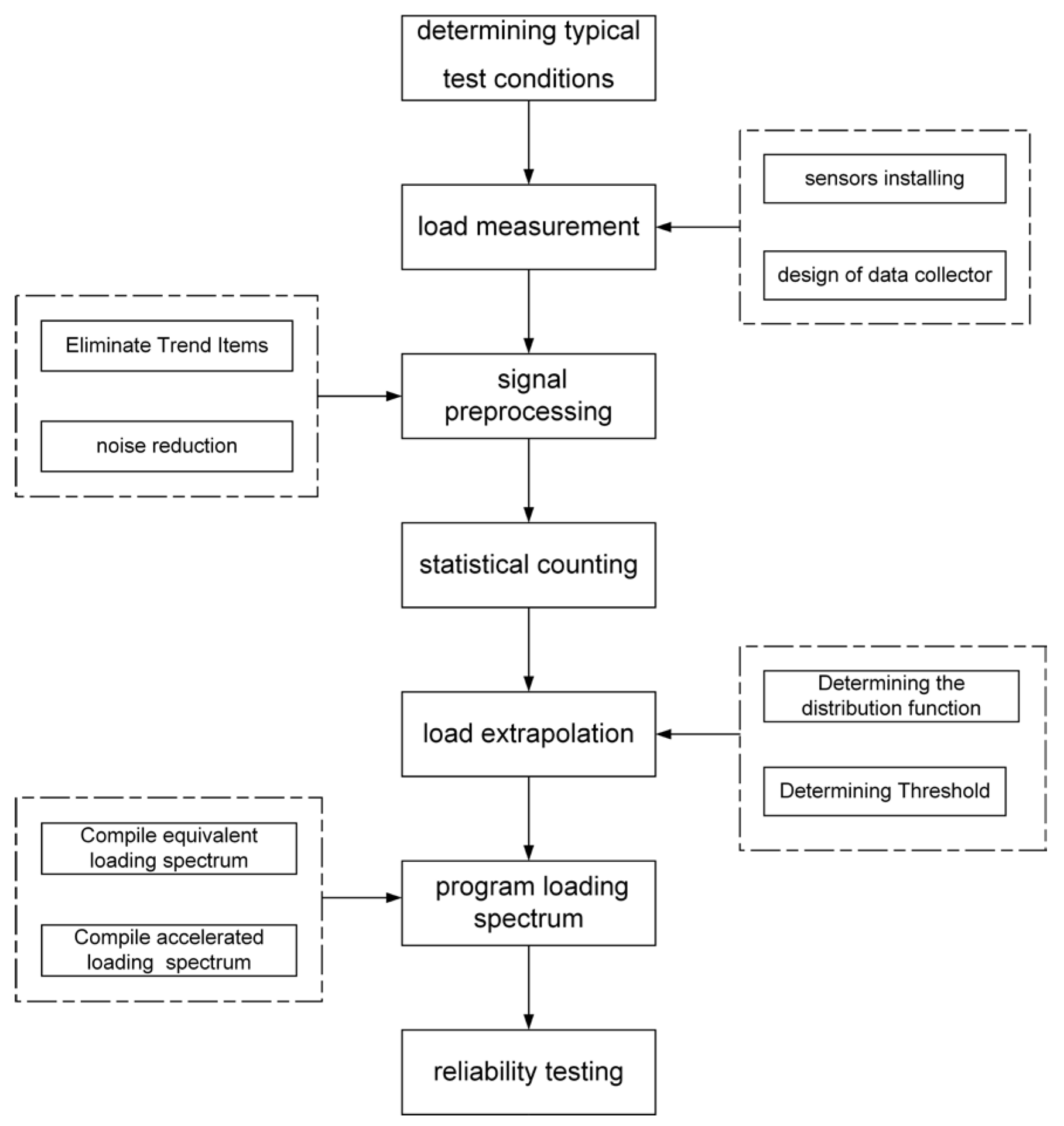
2.1. Load Spectrum Extrapolation Principle and Process

Using the time-domain load extrapolation method, the preprocessed time-domain load data is directly extrapolated to obtain the long-term load time history. The extreme load is the center of gravity for extrapolation, and the tail data of load distribution is mainly described through extreme value theory [21]. The process of time-domain load extrapolation mainly includes the following: removing small cycles from time-domain load data and extracting inflection points of extreme values; selecting an appropriate extreme load model and establishing an extreme load distribution model; and randomly generating a new time-domain extreme load sequence using the extreme load distribution to obtain extrapolated long-term time-domain loads. According to different extreme value models, common time-domain load extrapolation methods can be divided into time-domain extrapolation based on the BMM (Block Maximum Method) model, time-domain extrapolation based on the POT model, and time-domain extrapolation based on the MIS (Management Information System) model.

The process of load spectrum extrapolation is shown in Figure 1, which mainly includes the following steps: determining typical test conditions, load measurement, signal preprocessing, statistical counting [22], load extrapolation, program loading spectrum, and reliability testing.

2.2. Collection and Data Preprocessing of Traction Resistance Load Signal

2.2.1. Collection of Traction Resistance Load Signal

The experimental site for collecting traction resistance load signals is located in Liuhe District, Nanjing City, Jiangsu Province (Figure 2a). The soil specific resistance was about 3.5–4 N/cm² and the experiment area was 5000 m². The Dongfeng DF1004 tractor is taken as the research object, and the tractor’s three-point suspension is connected to the L1-435 moldboard plow to collect traction resistance signals under plowing conditions. The details of plow connection and sensor layout are shown in Figure 2b. The sensor adopts the XZNJNY-T3d30 KN electric quantity weighing sensor produced by Ningbo Keli Sensing Technology Co., Ltd. Ningbo China. This sensor is a pin-type force sensor, arranged at the pull-down rod of the three-point suspension device and collects the tractor traction resistance load signal through a wired collection system. The field test and sensor layout are shown in Figure 2. The technical specifications of the tractor, the sensor, and the moldboard plow are shown in

Table 1. The technical specifications of the sensor.

Name of Part	Parameter	Parameter Value
The tractor	Model name	DF1004X
	Outer dimension (mm × mm × mm)	4555 × 2270 × 2775
	Wheel pitch (Front wheel mm/rear wheel mm)	1550–2010, 1650
	Engine-calibrated power (kW)	73.5
	Minimum ground spacing (mm)	425
	Minimum service quality (kg)	4340
	Power output shaft power (kW)	63
The sensor	Model name	XZNJNY-T3d30 KN
	Supply voltage (V)	12
	Output signal (V)	2.5–4.5
The moldboard plow	Model name	1L-435
	Matching power (kW)	66.1–88.2
	Outer dimension (mm × mm × mm)	3400 × 1650 × 1350 mm
	Total weight (kg)	1050
	Depth range (mm)	200–350
	Plow number	4
	Adjustable range of total tillage (mm)	1400
	Plow spacing (mm)	880
	Operating speed (km/h)	8–12
	Matching tire spacing (mm)	1700–1900
	Connection type	three-point suspension

[23].

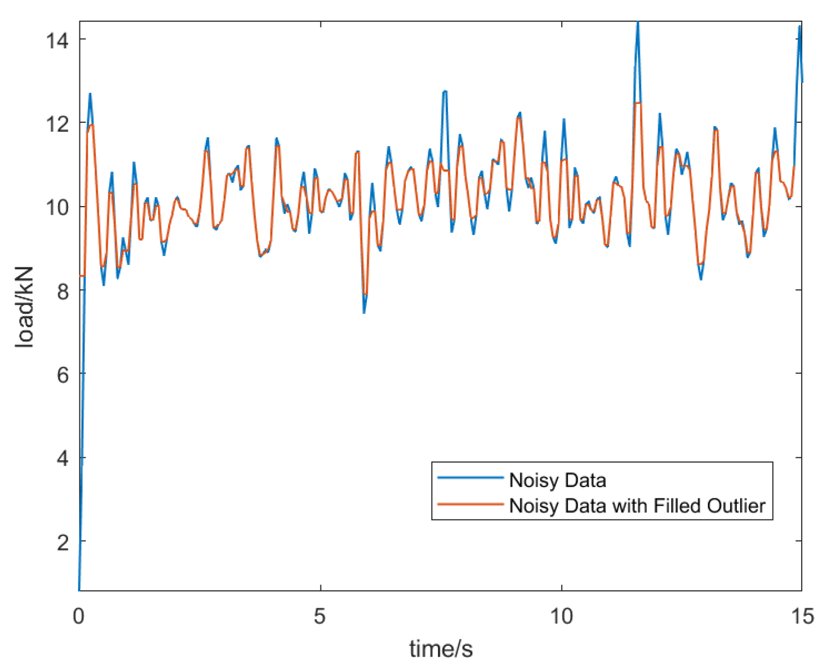
2.2.2. Preprocessing of Traction Resistance Load Signal

According to the traction resistance data of the three-point suspension system collected from field experiments, the original load signal can be obtained by processing the data, as shown in Figure 3.

Due to the complex field environment, there may be interference signals in the measured load signals during field experiments. If the original data is directly used to compile the load spectrum, the reliability of the compiled load spectrum will not be very high. Therefore, for the original load signal of tractor traction resistance collected by the testing system, preprocessing is necessary, and the processed signal needs to be verified and prepared for the compilation of load spectra for subsequent tractor field operations [24].

The collected raw signal data Itself has a certain range of oscillations, and in addition, there may be some low-frequency components that affect our calculations or observations. The polynomial least squares method is used to eliminate the trend term from the original load signal, and the results are shown in Figure 4.

Due to the harsh working conditions in the field, there are some abnormal peaks in the lines drawn after dispersion due to external interference or human error during the tractor field test. In order to obtain true and reliable load data, outlier of the original signal should be detected and smoothed before spectrum compilation, and the abnormal peaks should be eliminated [25,26], and the results are shown in Figure 5.

2.3. Extrapolation of Traction Resistance Load Spectrum

2.3.1. Determine the Distribution Function

Assuming $\left\{x_i\right\}(i=1,2,\dots ,n)$ is the load spectrum sample data, and its distribution is F (x). For a specific threshold, samples that are greater than the threshold are referred to as over-threshold samples, and $z_i=x_i-\mu (i=1,2,\dots ,n)$ is the excess amount. The distribution functions of the exceeding amount and exceeding threshold are shown in Equations (1) and (2), respectively:

$$F_{\mu }(z)=P\left\{X-\mu \le z|X\ge \mu \right\}=\frac{P\left\{\mu \le X-\mu \le z\right\}}{X\ge \mu }=\frac{F(z+\mu )-F(\mu )}{1-F(\mu )},z\ge 0$$

(1)

$$F_{\mu }(x)=P\left\{X\le x|X\ge \mu \right\}==\frac{F(x)-F(\mu )}{1-F(\mu )},x\ge \mu$$

(2)

According to the load characteristic analysis data, the threshold’s candidate interval is [7.898, 12.47] kN. Research has shown that the excess distribution tends to follow the generalized Pareto distribution (GPD) when the threshold is sufficiently large. Therefore, this article fits the excess distribution based on the GPD distribution.

The expression for the GPD cumulative distribution function is:

$$G(z,\mu ,\sigma ,\xi )=\{\begin{array}{l}1-{(1+\xi \frac{z}{\sigma })}^{-\frac{1}{\xi }},\xi \ne 0,x>\mu \\ 1-\exp (-\frac{z}{\sigma }),\xi =0,x>\mu \end{array}$$

(3)

The expression of the GPD probability density function is:

$$g(z,\mu ,\sigma ,\xi )=\{\begin{array}{l}\frac{1}{\sigma }{(1+\xi \frac{z}{\sigma })}^{-\frac{1+\xi }{\xi }},\xi \ne 0,x>\mu \\ \frac{1}{\sigma }\exp (-\frac{z}{\sigma }),\xi =0,x>\mu \end{array}$$

(4)

In the equation, $z_i=x_i-\mu (i=1,2,\dots ,n)$ is the excess, $x_i$ (kN) is the observed load value, $\mu$ (kN) is the threshold value, $\sigma$ is the scale parameter, and $\xi$ is the shape parameter.

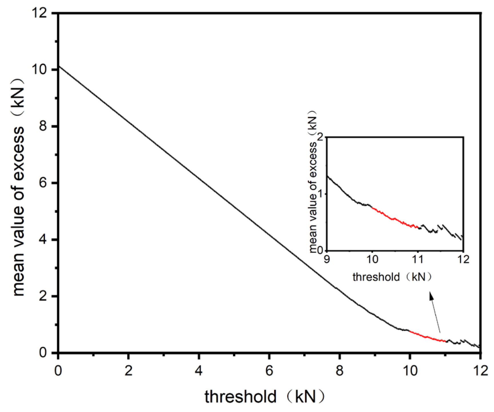
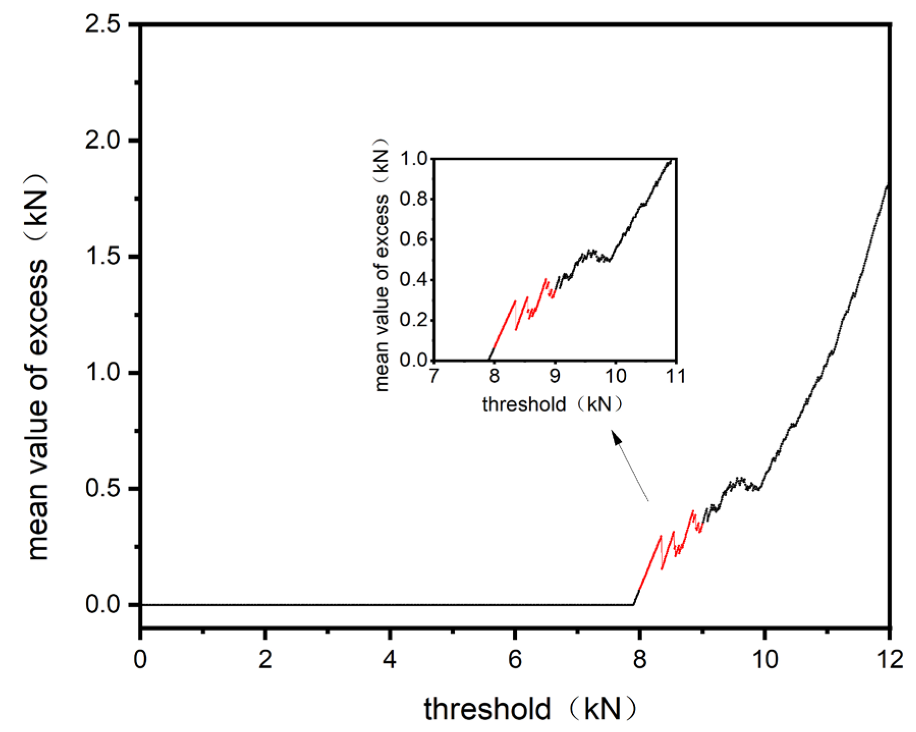
2.3.2. Determining the Threshold

The mean function of the excess of the random variable X is defined as $e\left(\mu \right)$, and its expression is:

$$e(\mu )=E(x-\mu |X>\mu )=\frac{\sigma +\xi \mu }{1-\xi }$$

(5)

When the scale parameter $\sigma$ and shape parameter $\xi$ are determined, there is a linear relationship between $e\left(\mu \right)$ and the threshold. Each threshold has a mean of the excess corresponding to it, as shown in Equation (6).

$$e_n(\mu )=\frac{1}{N}{\displaystyle \sum _{i=1}^n{X}_i}-\mu$$

(6)

In the formula, $\mu$ is the threshold, and N is the number of excess samples.

The graph of the mean function of the upper threshold exceedance is shown in Figure 6:

From the graph, it can be seen that as the threshold increases, the tail means oscillates violently. The linear change interval [10.10, 11.00] that is closest to the oscillation before the oscillation is selected as the initial upper threshold interval.

Similarly, the graph of the mean function of threshold exceedance can be obtained, as shown in Figure 7, with [8.50, 9.50] as the initial threshold interval.

• Threshold selection method based on grey correlation analysis;

Grey correlation analysis is a common threshold selection method. Grey correlation analysis is used to quantify the goodness of fit of the GPD distribution of excess quantities with different thresholds. The greater the grey correlation, the better the fitting effect [27]. The correlation analysis process is as follows [28]:

(1)

Given an alternative threshold, the corresponding excess sample data, and GPD fitting data are shown in Equation (7).

$$\{\begin{array}{l}f(x_i)=f_1,f_2,\cdots ,f_n\\ \widehat{f}(x_i)={\widehat{f}}_1,{\widehat{f}}_2,\cdots ,{\widehat{f}}_n\end{array},(i=1,2,3,\cdots ,n)$$

(7)

In the formula, $f\left(x_i\right)$ is the quantile of the sample point distribution of the original load data, $\widehat{f}\left(x_i\right)$ is the quantile of the fitting GPD distribution, and n is the number of excess samples.

(2)

Using the averaging method to $\widehat{f}\left(x_i\right)$ perform dimensionless processing on the load sample data $f\left(x_i\right)$ and fitting data, as shown in (8).

$$\{\begin{array}{l}f(x_i)=\frac{f_i}{{\displaystyle \sum _{i=1}^n{f}_i/n}}\\ \widehat{f}(x_i)=\frac{{\widehat{f}}_i}{{\displaystyle \sum _{i=1}^n{\widehat{f}}_i/n}}\end{array},(i=1,2,3,\cdots ,n)$$

(8)

(3)

Calculate the absolute difference between the sample and the fitted data after normalization and calculate the correlation coefficient based on the extreme values.

$$\Delta (x_i)=\left|\widehat{f}(x_i)-f(x_i)\right|$$

(9)

$$\{\begin{array}{l}M=\max (\Delta (x_i))\\ m=\min (\Delta (x_i))\end{array}$$

(10)

$$\omega (x_i)=\frac{m+\eta M}{\Delta (x_i)+\eta M}$$

(11)

In the formula, $\mathsf{\Delta }\left(x_i\right)$ is the absolute difference, $\eta$ is the resolution coefficient, and is taken as $\eta =0.5$.

(1)

Calculate alternative thresholds μ Corresponding grey correlation degree λ.

$$\lambda (\mu )=\frac{1}{n}{\displaystyle \sum _{i=1}^n\omega (x_i)}$$

(12)

• Optimal threshold selection based on genetic algorithm;

The threshold obtained by using the grey correlation analysis method was calculated using only 10 data points to reduce computational complexity. Therefore, this method’s accuracy of the threshold obtained is relatively low. This section uses genetic algorithm to optimize threshold selection and find the optimal threshold. The process is as follows [29]:

(2)

Determine the threshold range and initialize the population. The sample accuracy of the input data is 10⁻². If the input data is converted into binary encoding, the encoding length of the individual is:

$$l_G=1+{\log }_2\frac{({\mu }_2-{\mu }_1)}{eps}$$

(13)

In the formula, $l_G$ is the data encoding length, $eps$ is the sample accuracy, ${\mu }_1$ and ${\mu }_2$ is the upper and lower intervals of the initial threshold range.

(3)

Calculate individual fitness. Individual fitness is the survival probability of an individual under given environmental conditions. Based on the optimization objective, select the fitness function as the “environmental condition” in the genetic algorithm. This article aims to find the threshold that best fits the GPD function. Therefore, the goodness of fit of each candidate threshold is calculated as the fitness of the individual in the “environment”. This paper takes the grey relational degree as the fitness function. The greater the grey relational degree, the higher the probability that individuals can survive in the environment and pass on genes to the next generation and vice versa.

(4)

Individual survival rate. The survival rate of individuals in the environment is essentially the principle of “survival of the fittest” proposed by evolutionary theory. According to the choice function, the individuals with high fitness will have a higher survival rate, and the good genes will be passed on to the next generation, whereas the inferior genes in the population will be eliminated. The common roulette wheel method is selected as the choice function, in which the survival rate of each individual in the population is proportional to its fitness.

$$p(i)=\frac{f_g(i)}{{\displaystyle \sum _{j=1}^N{f}_i(x_j)}}$$

(14)

In the formula, $f_g\left(i\right)$ (i = 1,2,3…, n) is the fitness of each individual in the population, and $p\left(i\right)$ is the survival probability of the i-th individual in this inheritance.

(5)

Intersection and variation. The crossover and mutation process in genetic algorithms simulates the pairing and mutation of two pairs of chromosomes in nature. During the crossover process, two sets of data exchange “chromosomes” through certain crossover methods to form new individuals. This article adopts a single-point crossover. Mutation refers to the phenomenon where a certain “gene” within the data has a certain probability of being transformed into an opposite gene.

2.4. Equivalence of Traction Resistance Load Signal

The load spectrum obtained from the GPD distribution cannot directly guide the reliability tests related to plowing operations and the fatigue life prediction of key functional components. In order to facilitate the loading of the test bench, the principle of equal damage can be adopted to convert the load spectrum of each working stage into a constant stress spectrum. Then, according to the test requirements, the loading time of each working stage can be reasonably divided to obtain the loading curve of each cycle, which is called the loading spectrum [30,31].

Miner fatigue theory believes that each pressure applied to a part will cause certain damage to the part, and the magnitude of the damage is determined by the combined magnitude of the applied stress and the characteristics of the material itself [32]. When the damage accumulates to a certain value, the part fails, and vice versa, no failure occurs. The expression is:

$$D={\displaystyle \sum _i\frac{n_i}{N_i}}$$

(15)

Among them, D is the amount of damage, and $D\in \left[\mathrm{0,1}\right)$ when the part does not fail. When D = 1, the part experiences fatigue failure. $n_i$ is the $S_i$ number of loadings under stress $S_i$, and $N_i$ is the number of loadings where fatigue damage occurs under the equivalent force. The expression for $N_i$ is:

$$N_i=C{S}_i{}^{-\beta }$$

(16)

where C is a constant and β is the inverse slope coefficient of the material S-N curve, which is related to the material’s own properties, β = 7.1 [33,34].

From Equations (15) and (16), the equivalent loading stress $S_k$ and equivalent loading frequency n expressions can be obtained as:

$$S_k=\sqrt[\beta ]{\frac{{\displaystyle \sum _{i=1}^n{n}_i{S}_i{}^{\beta }}}{n}}$$

(17)

$$n=\frac{{\displaystyle \sum _{i=1}^n{n}_i{S}_i{}^{\beta }}}{S_k{}^{\beta }}$$

(18)

where $S_k$ is the equivalent loading stress, n is the equivalent loading frequency, $S_i$ is the load spectrum extrapolation data, and $n_i$ is the frequency of loading stress.

3. Results and Discussions

3.1. Load Characterization and Smoothness Testing after Pre-Processing

The load characteristics before and after pretreatment are shown in

Table 2. Comparison of characteristics before and after load signal preprocessing.

	Minimum /kN	Maximum /kN	Mean /kN	Median /kN	Std /kN	Range /kN
Before	0.7946	14.44	10.22	10.2	1.232	13.65
After	7.898	12.47	10.2	10.16	0.8382	4.57

. By comparing the data in Table 2, the data of maximum and minimum values before and after preprocessing changed significantly, which is due to the elimination of abnormal spikes during our preprocessing, and the variance and standard deviation were reduced after preprocessing, which indicates the good noise reduction effect of preprocessing. The mean and median values remain unchanged, which indicates that the data characteristics of the original load signal are also well preserved after preprocessing.

Using the adtest function in MATLAB, the ADF test (Augmented Dickey–Fuller test) can be performed on the smoothness of the load signal. The function’s output is “1”, and the test proves that the pre-processed load signal is smooth.

3.2. Threshold Selection Results and Analysis

3.2.1. Threshold Selection Method Based on Grey Correlation Analysis

Based on the initial range of upper and lower thresholds obtained by the image method, 10 thresholds are selected at equal intervals, and the gray correlation degree is calculated. The gray correlation degrees of different thresholds are shown in

Table 3. Grey correlation degree corresponds to each threshold within the threshold interval.

Upper Threshold		Lower Threshold
Threshold/kN	Gray Correlation	Threshold/kN	Gray Correlation
10.10	0.6763	8.60	0.6942
10.20	0.6762	8.70	0.6630
10.30	0.6855	8.80	0.7153
10.40	0.6788	8.90	0.6443
10.50	0.6887	9.00	0.6962
10.60	0.6832	9.10	0.6738
10.70	0.7005	9.20	0.6598
10.80	0.7092	9.30	0.7001
10.90	0.7182	9.40	0.6620
11.00	0.7173	9.50	0.6540

below.

Based on the calculation results, the bolded thresholds in the red rectangular boxes in Table 3 were the best-fitting thresholds. The threshold interval was determined to be [8.80, 10.90] kN.

Using the extracted exceedance samples for parameter estimation, the exceedance samples were fitted to the GPD distribution using the great likelihood estimation method to find the corresponding scale parameter $\sigma$ and shape parameter $\xi$, as shown in

Table 4. GPD fitting results corresponding to threshold based on grey correlation analysis.

Threshold/kN	Scale Parameter σ	Shape Parameter ξ
8.80	117.7353	−1.3046
10.90	61.2523	−0.2479

[35].

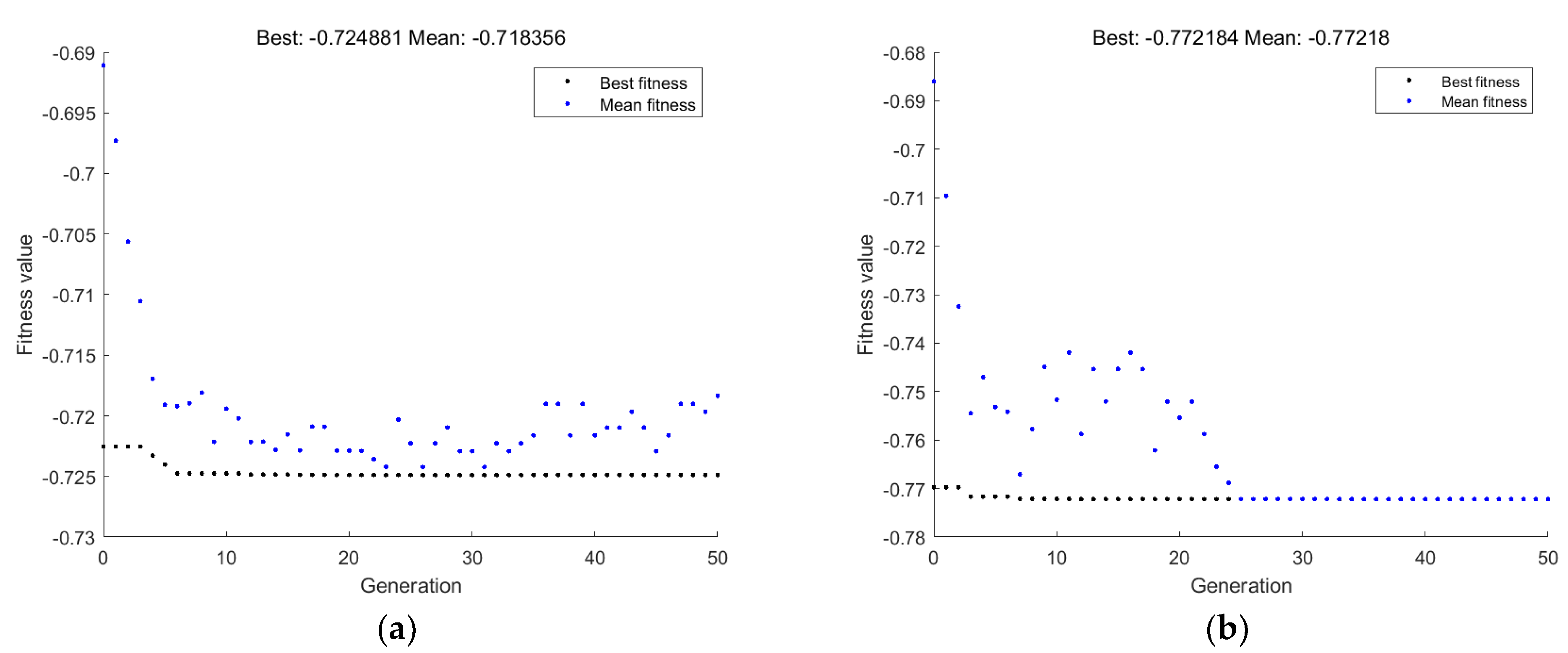
3.2.2. Optimal Threshold Selection Based on Genetic Algorithm

By writing the program in MATLAB, 50 iterations yielded an optimal upper threshold of 10.975 kN, at which time the gray correlation was 0.7249; the optimal lower threshold was 8.5455 kN, at which time the gray correlation was 0.7722, and the evolutionary process of the upper and lower threshold genetic algorithm is shown in Figure 8.

The comparison of the data with the gray correlation analysis method is shown in

Table 5. Thresholds and gray correlations obtained by the two methods.

	Upper Threshold/kN	Gray Correlation	Lower Threshold/kN	Gray Correlation
Threshold selection method based on grey correlation analysis	10.90	0.7182	8.80	0.7153
Threshold selection method based on genetic algorithm	10.9750	0.7249	8.5455	0.7722

. The results show that the gray correlation of the upper and lower thresholds selected by the genetic algorithm increased by 0.933% and 7.950%, respectively, compared with the traditional gray correlation analysis method, and the gray correlation of the thresholds obtained by this method was greater, indicating that the GPD fit of the threshold exceeded the amount was better.

Using the extracted exceedance samples for parameter estimation, the exceedance samples were fitted to the GPD distribution using the great likelihood estimation method to find the corresponding scale parameter $\sigma$ and shape parameter $\xi$, as shown in

Table 6. GPD fitting results corresponding to the optimal threshold.

Threshold/kN	Scale Parameter σ	Shape Parameter ξ
8.54558	146.8319	−0.4468
10.975	58.5881	−0.2369

.

After obtaining the scale parameter $\sigma$ and shape parameter $\xi$ for the upper and lower thresholds, the cumulative distribution functions and probability density functions corresponding to the upper and lower thresholds can be written:

$$\{\begin{array}{l}G(z,\mu ,\sigma ,\xi )=1-{(1-0.2369\frac{x-1097.5}{58.5881})}^{4.2212}\\ g(z,\mu ,\sigma ,\xi )=0.0171{(1-0.2369\frac{x-1097.5}{58.5881})}^{3.2212}\end{array}$$

(19)

$$\{\begin{array}{l}G(z,\mu ,\sigma ,\xi )=1-{(1-0.4468\frac{x-854.55}{146.8319})}^{2.2381}\\ g(z,\mu ,\sigma ,\xi )=0.0068{(1-0.4468\frac{x-854.55}{146.8319})}^{1.2381}\end{array}$$

(20)

The goodness of fit can be observed more visually by plotting the Q–Q plot (Quantile–Quantile) of the original sample points against the fitted sample points. As shown in Figure 9, the fitted data points for the upper and lower thresholds (as the blue crosses in the figure) have a slight deviation around the reference line at both ends, whereas in the middle region, they fit the reference line very well, and the Q–Q plot of the final fitted sample approximates a straight line, which indicates a good fit of GDP at this threshold.

3.3. Load Spectrum Extrapolation Reconstruction Results and Validation

Combined with the probability density function of the GPD fitted distribution of the excess amount, a random load sequence consistent with the number of samples is generated, and the extrapolated time-domain signal is obtained by replacing the original excess amount at the original time point with the generated load sequence [36,37]. The original load is compared with extrapolated time courses of 1×, 2×, and 10×, as shown in Figure 10.

The 10-time original load and 10-time extrapolated load are counted, and the comparison of the accumulated frequency data of 10-time original load and 10-time extrapolated load is shown in Figure 11. It can be seen that the changing trend of the accumulated frequency of extrapolated load and original load is basically the same, and this extrapolation method is reasonable.

The load spectra obtained by extrapolation and the original load spectra are counted separately for rainfall, and the mean frequency histogram can be obtained, as shown in Figure 12. The load cycle distribution obtained by extrapolation in the time domain has similarity with the original data load cycle distribution, and the correlation coefficients of its magnitude and mean value are 0.95913 and 0.99187, respectively, indicating that the load cycle distribution can better simulate the real distribution law of the load under the plowing-operation conditions of the tractor.

3.4. Plotting of Loading Spectra and Accelerated Loading Spectra

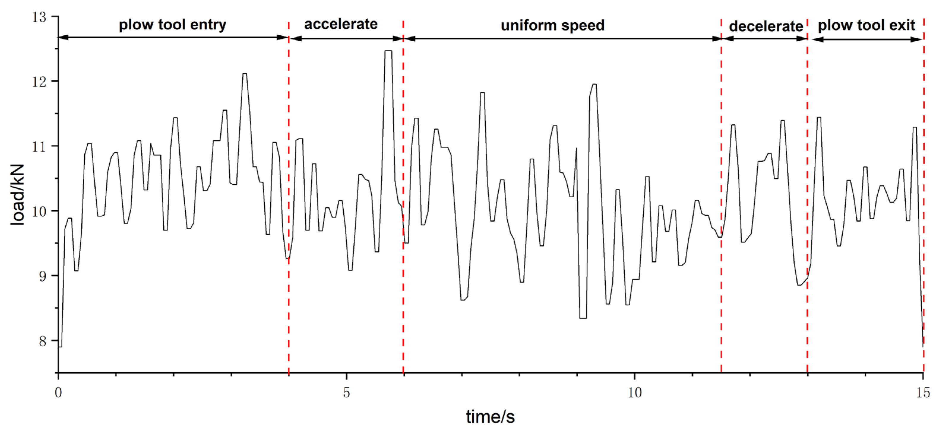
3.4.1. Analysis of the Plowing Process

The operating conditions of plowing operations consist of five stages: plow tool entry, accelerated operation, uniform speed operation, deceleration operation, and plow tool exit. The boundary of each working phase was distinguished by observing the change in load signal of each moving structure. The time consumption of each working stage is 4.1 s, 1.9 s, 5.6 s, 1.6 s, and 1.8 s. The working stages are shown in Figure 13.

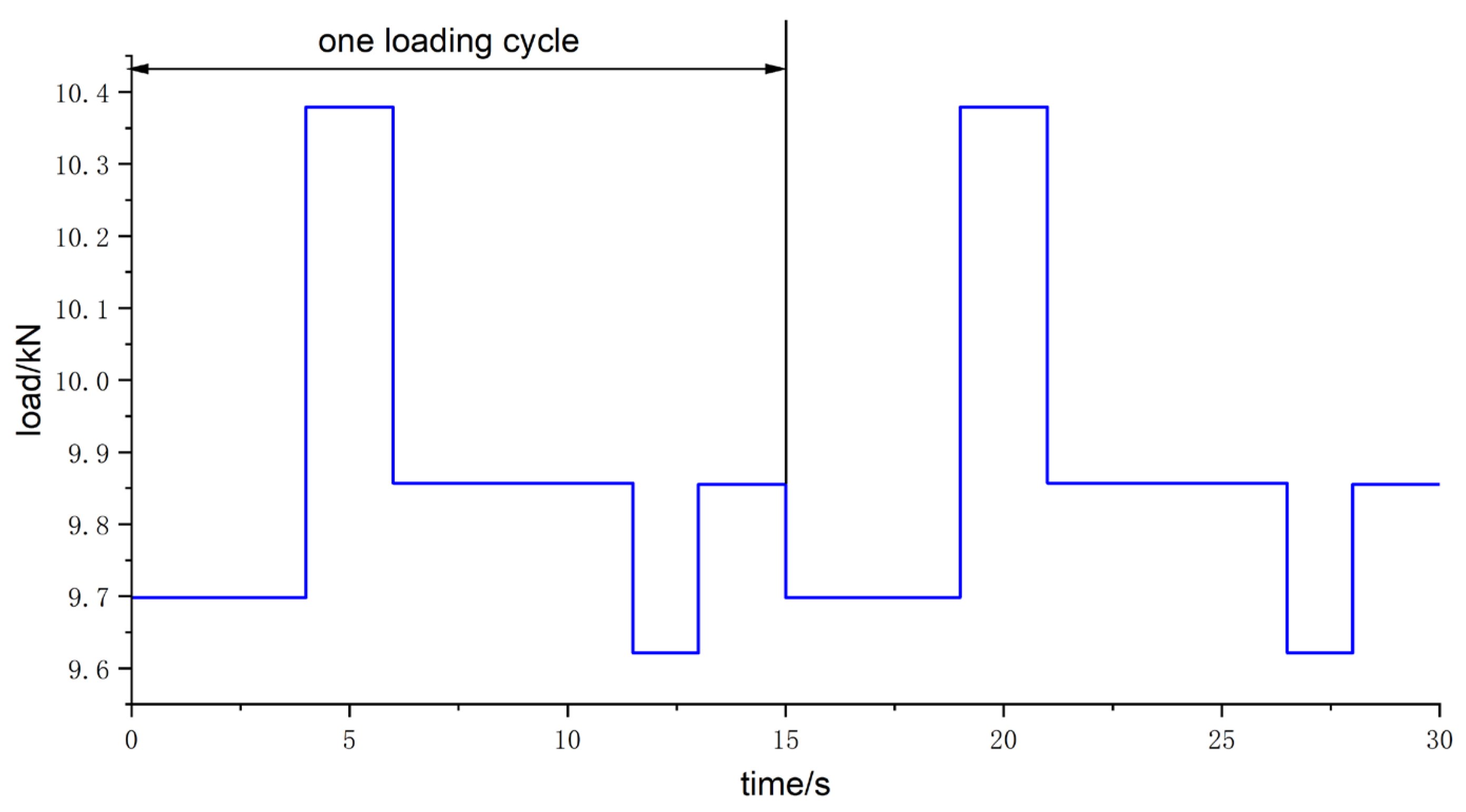
3.4.2. Division of Loading Loops

In order to facilitate the preparation of the subsequent loading spectra and the easy implementation of the test bench loading, the time periods were rounded, and the elapsed time of each working phase in one loading cycle is shown in

Table 7. Time consumption of each work stage.

	Plow Tool Entry	Accelerated Operation	Uniform Speed Operation	Deceleration Operation	Plow Tool Exit
Time/s	4	2	5.5	1.5	2

.

Preparing the loading spectrum requires the calculation of equivalent loading stresses for each working stage and the extrapolation of the load spectrum for rainflow counting statistics. According to the literature, the load level divided into 8 levels can accurately reflect the fatigue characteristics of the material, so the amplitude load interval of each working stage of the plowing load is divided into 8 levels with the ratio coefficients of 0.125, 0.275, 0.425, 0.575, 0.725, 0.850, 0.950, and 1.000 [38]. The amplitude equivalent of different working stage load spectrum is shown in

Table 8. Amplitude Equivalent Load Spectrum.

		1	2	3	4	5	6	7	8
Plow tool entry	Amplitude/kN	0.4963	0.9925	1.4888	1.985	2.4813	2.9775	3.4738	3.9658
	Frequency	3	1	3	3	2	0	0	1
Accelerated operation	Amplitude/kN	0.4129	0.8258	1.2387	1.6512	2.0646	2.4774	2.8903	3.3032
	Frequency	1	2	2	0	0	1	1	0
Uniform speed operation	Amplitude/kN	0.4563	0.9125	1.3688	1.8250	2.2813	2.7375	3.1938	3.6412
	Frequency	12	1	5	0	2	1	2	1
Deceleration operation	Amplitude/kN	0.4380	0.8761	1.3141	1.7522	2.1902	2.6282	3.0663	3.5043
	Frequency	0	1	0	0	1	0	0	1
Plow tool exit	Amplitude/kN	0.4488	0.8975	1.3463	1.795	2.2438	2.6925	3.1413	3.5891
	Frequency	0	3	2	1	1	0	0	1

below.

According to the measured limited load data, the load cycle accumulation frequency is extended to 10⁶ times according to Equation (21) so as to obtain the extrapolation factor. Keeping the loading times constant, the loading times of each working stage after extrapolation are 236,364, 127,273, 436,364, 54,545, and 145,455, and the amplitude equivalent load spectrum after extrapolation is shown in

Table 9. Equivalent load spectrum of amplitude after frequency extrapolation.

		1	2	3	4	5	6	7	8
Plow tool entry	Amplitude/kN	0.4963	0.9925	1.4888	1.985	2.4813	2.9775	3.4738	3.9658
	Frequency	54,546	18,182	54,546	54,546	36,364	0	0	18,182
Accelerated operation	Amplitude/kN	0.4129	0.8258	1.2387	1.6512	2.0646	2.4774	2.8903	3.3032
	Frequency	18,182	36,364	36,364	0	0	18,182	18,182	0
Uniform speed operation	Amplitude/kN	0.4563	0.9125	1.3688	1.8250	2.2813	2.7375	3.1938	3.6412
	Frequency	218,182	18,182	90,909	0	36,364	18,182	36,364	18,182
Deceleration operation	Amplitude/kN	0.4380	0.8761	1.3141	1.7522	2.1902	2.6282	3.0663	3.5043
	Frequency	0	18,182	0	0	18,182	0	0	18,182
Plow tool exit	Amplitude/kN	0.4488	0.8975	1.3463	1.795	2.2438	2.6925	3.1413	3.5891
	Frequency	0	54,546	36,364	18,182	18,182	0	0	18,182

.

$$N_i{}^{\prime }/N_i={10}^6/N$$

(21)

where N is the total frequency of load, $N_i$ is the frequency of load in a certain operation phase, and ${N_i}^{\prime }$ is the frequency of load after expansion.

3.4.3. Preparation of Loading Spectra

The equivalent force of each working stage is calculated according to Equation (17), as shown in

Table 10. Equivalent stress at each working stage.

	Plow Tool Entry	Accelerated Operation	Uniform Speed Operation	Deceleration Operation	Plow Tool Exit
Time/s	4	2	5.5	1.5	2
Equivalent Amplitude/kN	2.799476	2.289872	2.565511	3.016759	2.694487
Equivalent Stress /kN	9.698	10.379	9.857	9.621	9.855

.

The loading spectrum is plotted according to the time consumed in each working phase and the equivalent force obtained from Table 9, as shown in Figure 14.

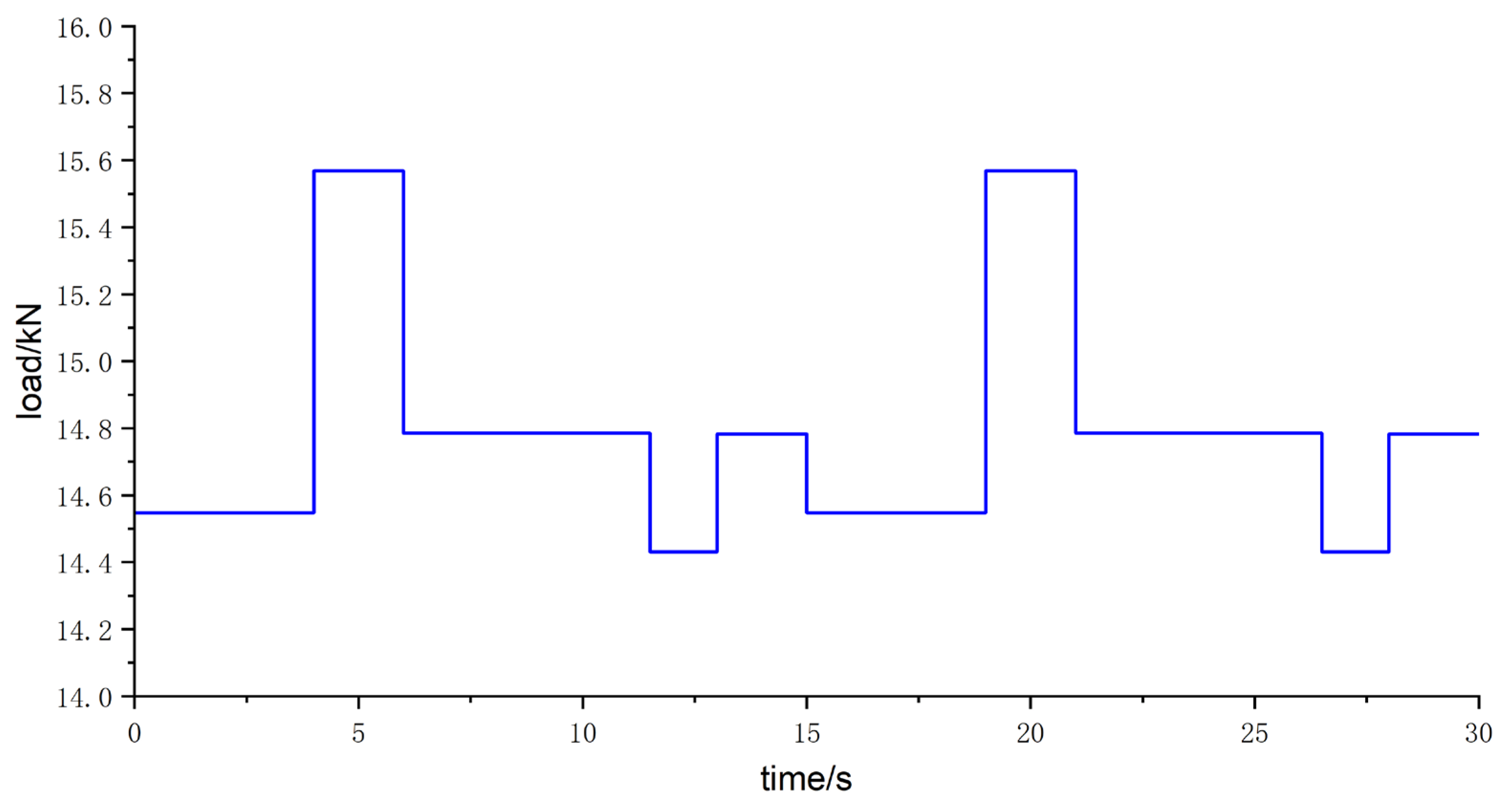
3.4.4. Development of Accelerated Loading Spectrum

The loading test is time-consuming, and the human, financial, and time costs are too great if the test is loaded directly. Therefore, choosing a suitable acceleration factor to accelerate the equivalent force and make the part fail quickly on the test bench is necessary.

The acceleration factor is related to the material of the part. The fatigue characteristics of the material can be described by the S-N curve, through the S-N curve can get the fatigue strength ratio $K_n$ of the part under different stresses. However, the material used in the process, as well as variations in its composition, can also influence the selection of the acceleration factor. To account for the inherent dispersion of the material, it is necessary to introduce the material dispersion correction factor, denoted as $K_v$. Therefore, it can be seen that the acceleration factor K can be expressed by the formula (22).

$$K=K_n{K}_v$$

(22)

where K is the acceleration factor, $K_n$ is the fatigue strength ratio of the material, 1.15, and $K_v$ is the discrete correction factor of the material, 1.3. Thus, it can be calculated that $K=1.5$ [39].

After the acceleration, the equivalent force of each working stage is shown in Table 10. The accelerated loading spectrum is plotted according to the time consumed in each working stage and the equivalent force obtained from

Table 11. Accelerated stress at each working stage.

	Plow Tool Entry	Accelerated Operation	Uniform Speed Operation	Deceleration Operation	Plow Tool Exit
Accelerated Stress/kN	14.547	15.5685	14.7855	14.4315	14.7825

, as shown in Figure 15.

Comparing Figure 14 and Figure 15, it can be seen that the waveforms of the accelerated loading spectrum are consistent with those before the acceleration, and only the accelerated stress of each section is raised to the loading stress. This shows that when using accelerated loading spectra for reliability testing on a test stand, the test time can be shortened while achieving the desired results, which greatly reduces human, financial and time costs.

4. Conclusions

From the above research and analysis, this paper concludes the following five points:

(1)

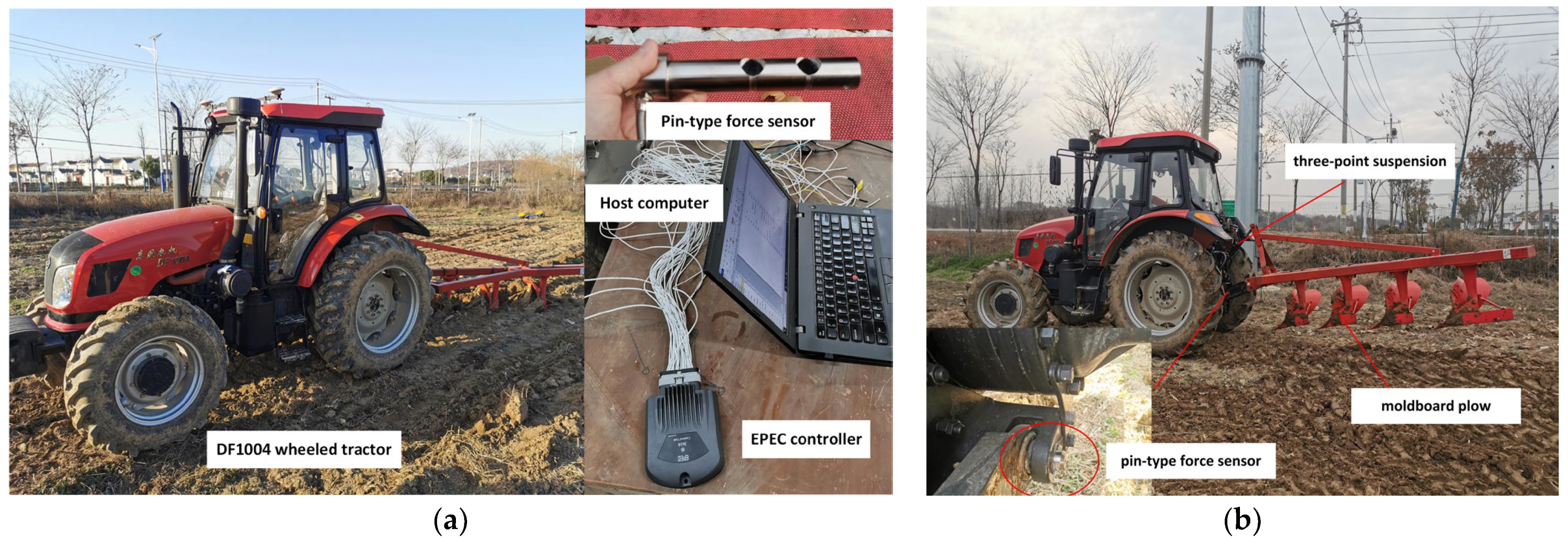
Taking the Dongfeng DF1004 tractor as the research object, the plowing operation was carried out in a test field with an area of about 5000 m², and the axle-pin force sensor was used to collect the traction resistance load signal of the three-point suspension device under the plowing condition. We stored sensor signals with the EPEC controller and transmitted them to the host computer. The foundation was laid for plotting the load time course curve later on;

(2)

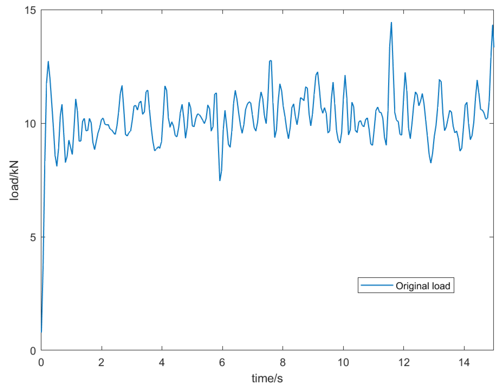
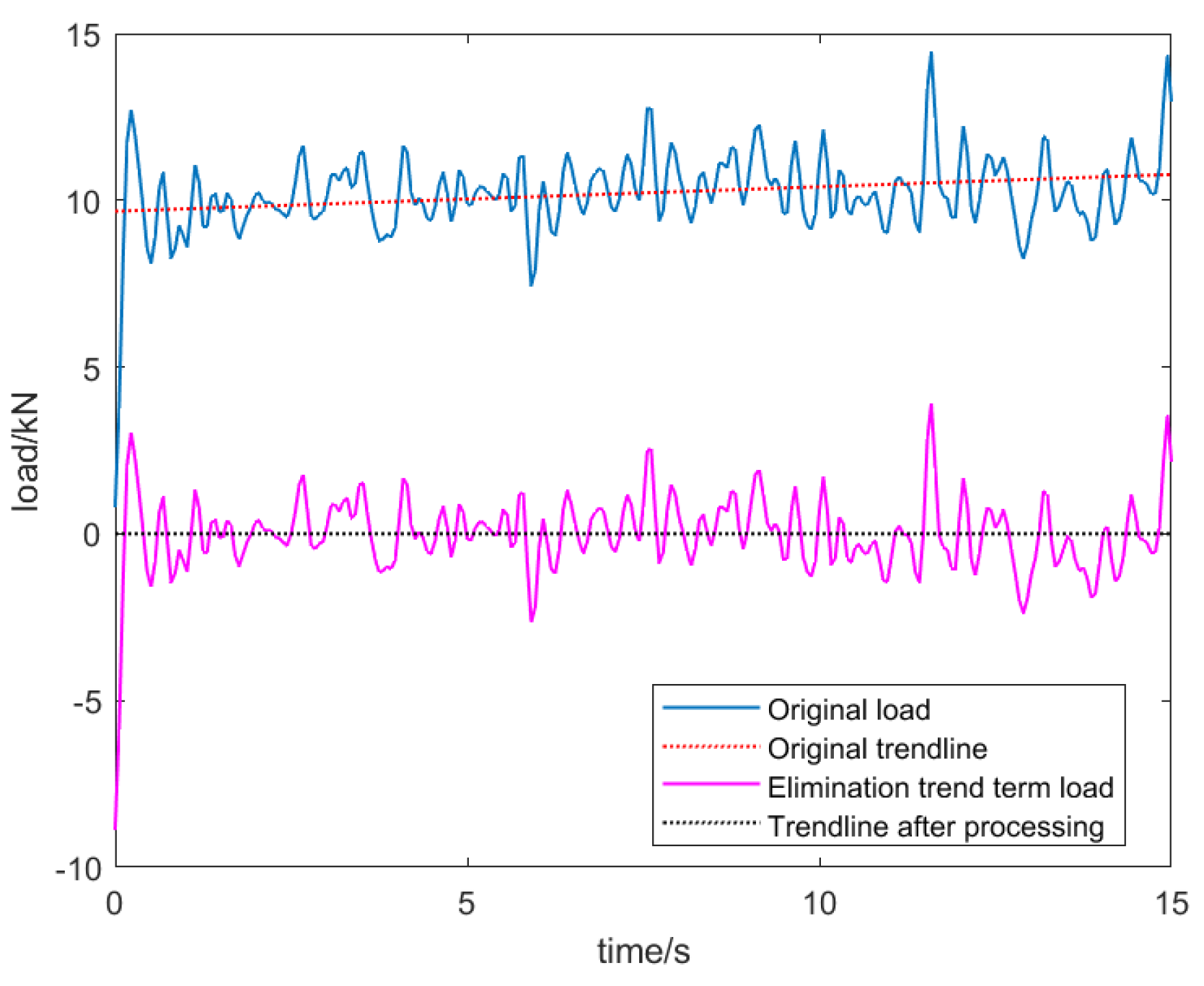
Based on the least squares method, the original load signal was processed by detrending, the data was noise-reduced by smoothing, and the smoothness of the pre-processed traction resistance load signal was verified by ADF test to obtain the original load time history of traction resistance under plowing conditions, which laid the foundation for the extrapolation and reconstruction of the load spectrum later on;

(3)

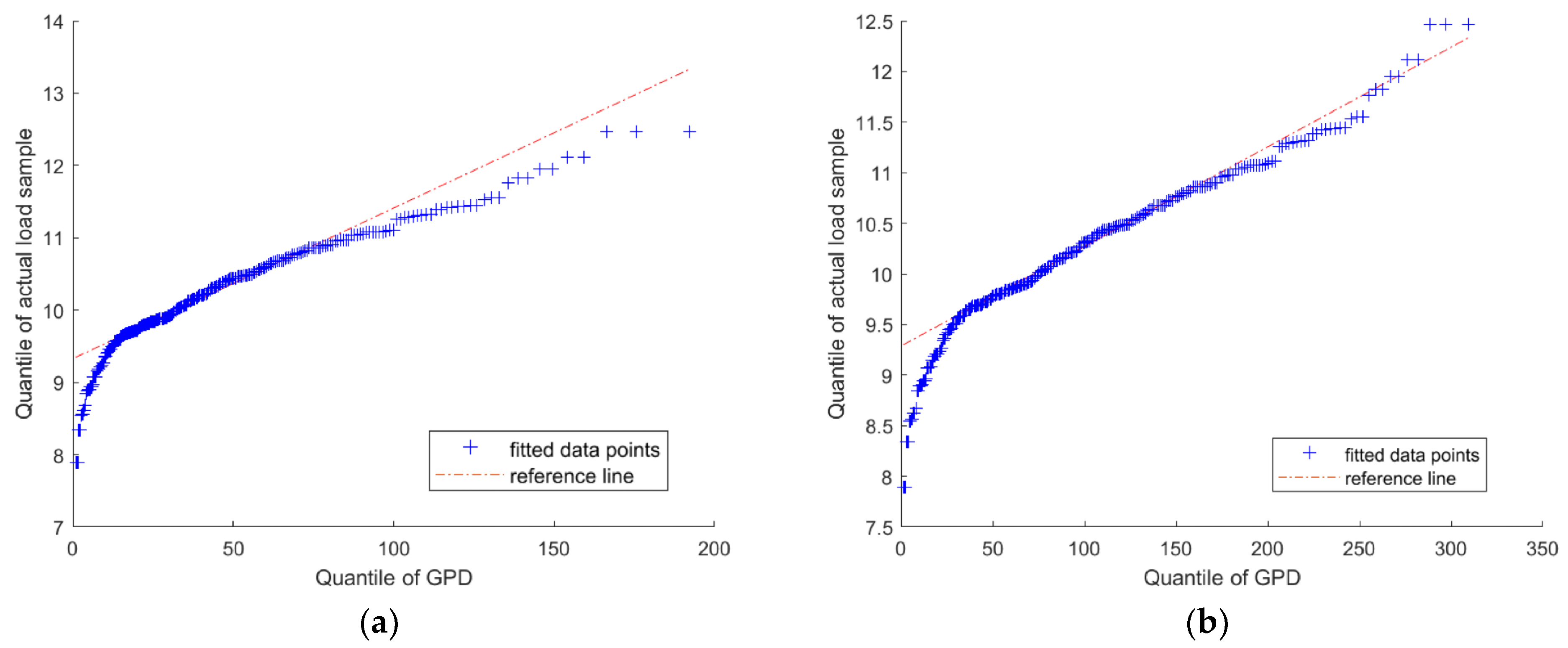
Based on the POT model, the time-domain extrapolation of the original load data is carried out, and the excess threshold values are selected using gray correlation analysis and genetic algorithm. The threshold values obtained are [8.80 kN, 10.90 kN] and [8.5455 kN, 10.975 kN], respectively, and the GPD distribution goodness-of-fit test is performed on the selected upper and lower thresholds. The fit superiority of the upper and lower thresholds obtained by the genetic algorithm is improved by 0.933% and 7.95%, respectively, which proves that the fitted curves obtained based on the optimal threshold selection of the genetic algorithm can better reflect the actual loading situation;

(4)

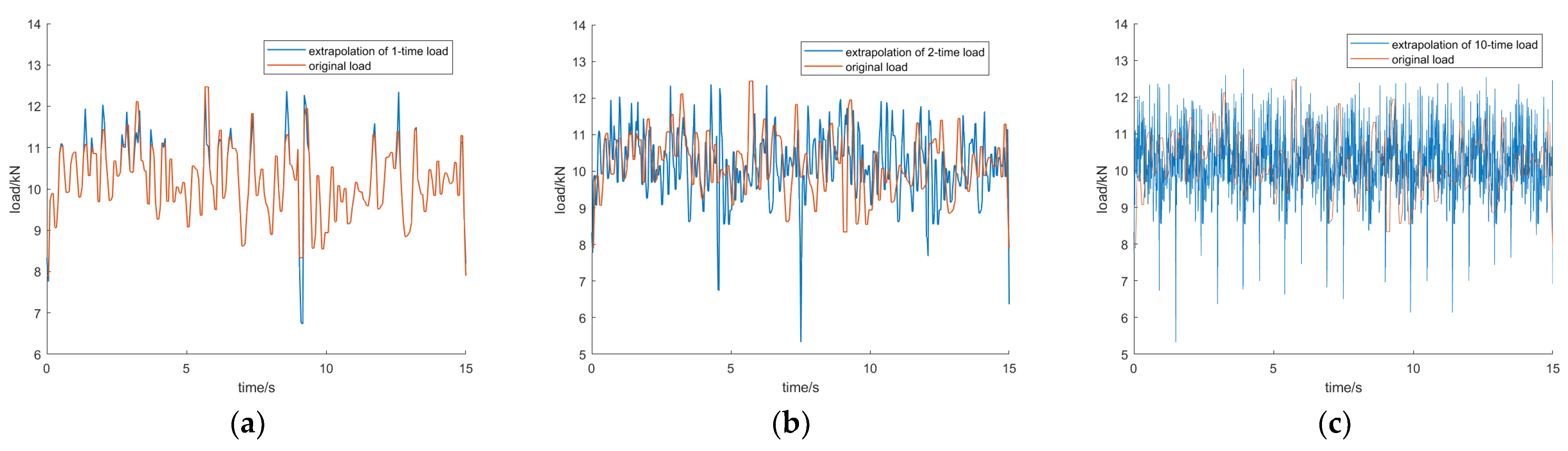
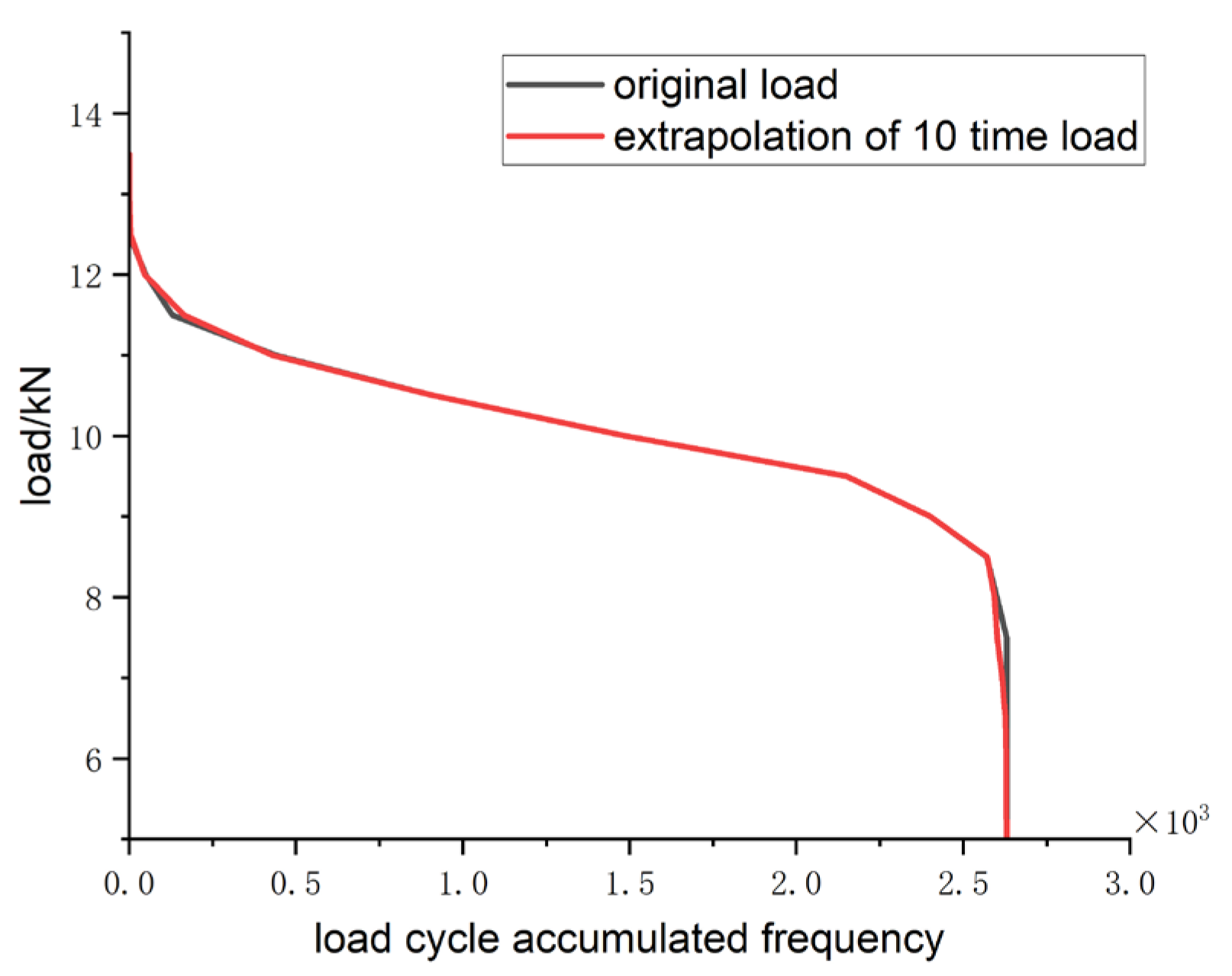
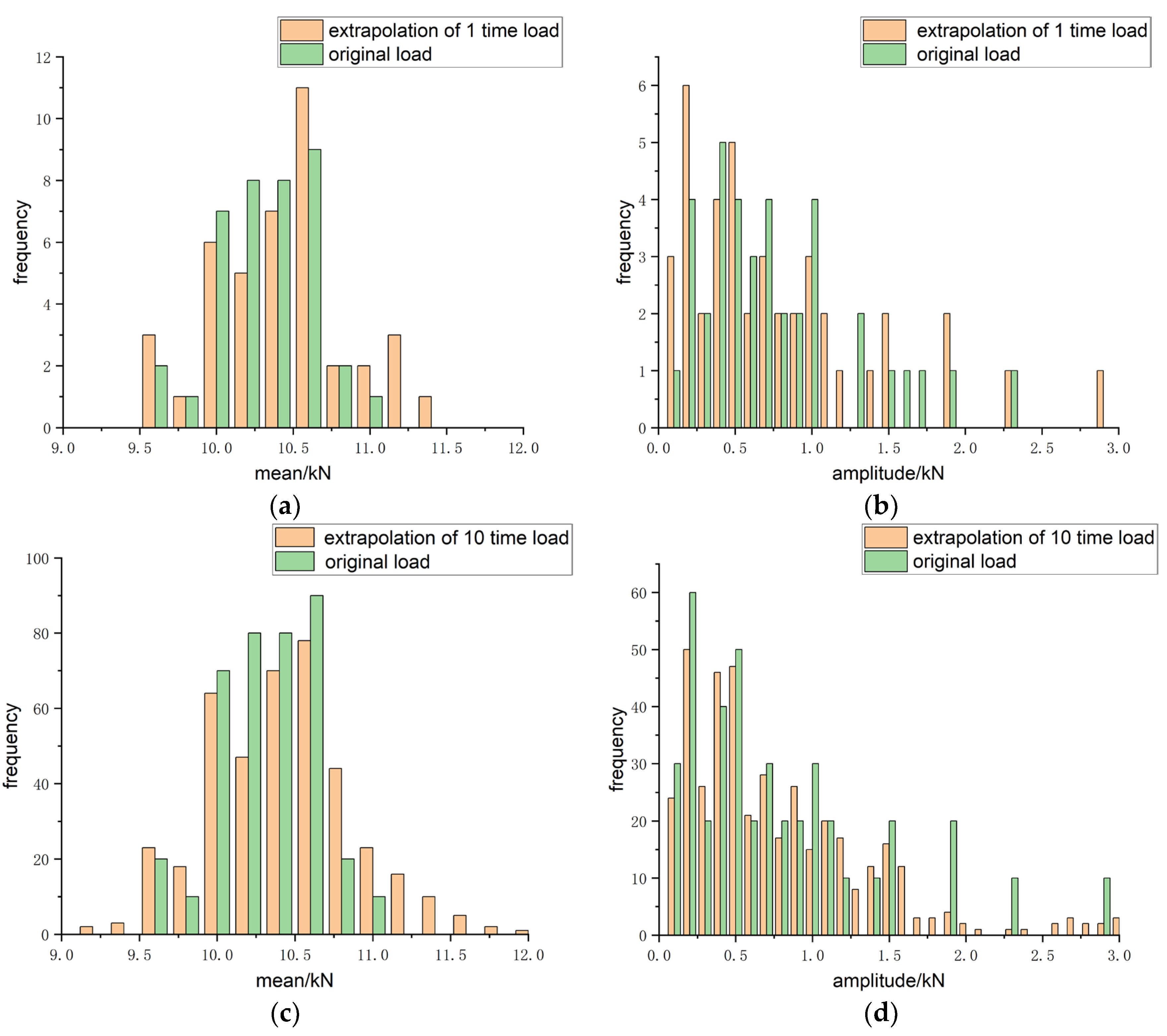
Based on the threshold thresholds obtained from the optimal threshold selection of the genetic algorithm, the original load time histories were extrapolated and reconstructed. The extrapolated load spectra obtained from the original load signal and 10-fold extrapolation were compared and analyzed by rain flow counting. The results show that the changing trend of the extrapolated load and the accumulated frequency of the original load are basically the same, and the extrapolation method is reasonable; the load cycle distribution obtained by time-domain extrapolation is similar to the load cycle distribution of the original data, and the correlation coefficients of its amplitude and mean value are 0.95913 and 0.99187, respectively. The load cycle distribution can better simulate the real load under the working condition of tractor plowing-distribution law;

(5)

The plowing condition is divided into five working stages: plow tool entry, accelerated operation, uniform speed operation, deceleration operation, and plow tool exit. The accumulated frequency of load cycles was extended to 106 times to obtain the amplitude equivalent load spectrum. Based on Miner fatigue theory, the equivalent force of each working stage was calculated, and the loading spectrum under plowing working conditions was drawn. Based on the accelerated life theory, the acceleration factor of 1.5 is obtained according to the S-N curve, and the accelerated loading spectrum under plowing conditions is finally drawn. The accelerated loading spectrum is consistent with the loading spectrum waveform, and only the stress is accelerated to the loading stress, which is convenient for loading on the test bench.

References

1. Zheng, G.; Wang, Q.; Cai, C. Criterion to determine the minimum sample size for load spectrum measurement and statistical extrapolation. Measurement 2021, 178, 109387. [Google Scholar] [CrossRef]
2. He, C. Research on Extrapolation and Compilation Method of Pressure Load Spectrum of Excavator Main Pump. Master’s Thesis, Jilin University, Jilin, China, 2022. [Google Scholar]
3. Wang, Q.; Zhou, J.; Gong, D.; Wang, T.; Sun, Y. Fatigue life assessment method of bogie frame with time-domain extrapolation for dynamic stress based on extreme value theory. Mech. Syst. Signal Process. 2021, 159, 107829. [Google Scholar] [CrossRef]
4. Shao, X.; Yang, Z.; Mowafy, S.; Zheng, B.; Song, Z.; Luo, Z.; Guo, W. Load characteristics analysis of tractor drivetrain under field plowing operation considering tire-soil interaction. Soil Tillage Res. 2023, 227, 105620. [Google Scholar] [CrossRef]
5. Tovo, R. A damage-based evaluation of probability density distribution for rain-flow ranges from random processes. Int. J. Fatigue 2000, 22, 425–429. [Google Scholar] [CrossRef]
6. Wang, Y.; Wang, L.; Lv, D.; Wang, S. Extrapolation of Tractor PTO Torque Load Spectrum Based on Automated Threshold Selection with FDR. Trans. J. Agric. Mach. 2021, 52, 364–372. [Google Scholar] [CrossRef]
7. Yang, Z.; Song, Z.; Luo, Z.; Zhao, X.; Yin, Y. Time-domain Load Extrapolation Method for Tractor Key Parts Based on EMD-POT Model. J. Mech. Eng. 2022, 58, 252–262. [Google Scholar] [CrossRef]
8. He, J.L.; Zhao, X.Y.; Li, G.F.; Chen, C.; Yang, Z.; Hu, L.; Xinge, Z. Time domain load extrapolation method for CNC machine tools based on GRA-POT model. Int. J. Adv. Manuf. Technol. 2019, 103, 3799–3812. [Google Scholar] [CrossRef]
9. Yang, Z.H.; Song, Z.H.; Zhao, X.Y.; Zhou, X. Time-domain extrapolation method for tractor drive shaft loads in stationary operating conditions. Biosyst. Eng. 2021, 210, 143–155. [Google Scholar] [CrossRef]
10. Yang, Z.; Song, Z.; Yin, Y.; Zhao, X.; Liu, J.; Han, J. Time domain extrapolation method for load of drive shaft of high-power tractor based on POT model. Trans. Chin. Soc. Agric. Eng. 2019, 35, 40–47. [Google Scholar] [CrossRef]
11. Dai, D.; Chen, D.; Wang, S.; Li, S.; Mao, X.; Zhang, B.; Wang, Z.; Ma, Z. Compilation and Extrapolation of Load Spectrum of Tractor Ground Vibration Load Based on CEEMDAN-POT Model. Agriculture 2023, 13, 125. [Google Scholar] [CrossRef]
12. Wang, Y.; Wang, L.; Zong, J.; Lv, D.; Wang, S. Research on Loading Method of Tractor PTO Based on Dynamic Load Spectrum. Agriculture 2021, 11, 982. [Google Scholar] [CrossRef]
13. Wang, L.; Zong, J.; Wang, Y.; Fu, L.; Mao, X.; Wang, S. Compilation and bench test of traction force load spectrum of tractor three-point hitch based on optimal distribution fitting. Trans. Chin. Soc. Agric. Eng. 2022, 38, 41–49. [Google Scholar] [CrossRef]
14. Johannesson, P. Extrapolation of load histories and spectra. Fatigue Fract. Eng. Mater. Struct. 2006, 29, 201–207. [Google Scholar] [CrossRef]
15. Yang, X.; Liu, X.; Tong, J.; Wang, Y.; Wang, X. Research on load spectrum construction of bench test based on automotive proving ground. J. Test. Eval. 2018, 46, 244–251. [Google Scholar] [CrossRef]
16. Yang, X.; Zhang, J.; Ren, W.X. Threshold selection for extreme strain extrapolation due to vehicles on bridges. Procedia Struct. Integr. 2017, 5, 1176–1183. [Google Scholar] [CrossRef]
17. Johannesson, P.; Thomas, J.J. Extrapolation of rainflow matrices. Extremes 2001, 4, 241–262. [Google Scholar] [CrossRef]
18. Wang, M.; Liu, X.; Wang, X.; Wang, Y.S. Research on load spectrum construction of automobile key parts based on monte carlo sampling. J. Test. Eval. 2018, 46, 1099–1110. [Google Scholar] [CrossRef]
19. Nagode, M.; Fajdiga, M. A general multi-modal probability density function suitable for the rainflow ranges of stationary random processes. Int. J. Fatigue 1998, 20, 211–223. [Google Scholar] [CrossRef]
20. Yu, L.; An, Y.; He, J.; Li, G.; Wang, S. Research Progress and Development Trend of Load Spectrum Extrapolation Technology for Mechanical and Electrical Equipment. J. Jilin Univ. Eng. Technol. 2023, 53, 941–953. [Google Scholar] [CrossRef]
21. Marty, C.; Blanchet, J. Long-term Changes in Annual Maximum Snow Depth and Snowfall in Switzerland Based on Extreme Value Statistics. Clim. Change 2012, 111, 705–721. [Google Scholar] [CrossRef]
22. Shao, X.; Song, Z.; Yin, Y.; Xie, B.; Liao, P. Statistical Distribution Modelling and Parameter Identification of the Dynamic Stress Spectrum of a Tractor Front Driven Axle. Biosyst. Eng. 2021, 205, 152–163. [Google Scholar] [CrossRef]
23. Wen, C.; Xie, B.; Song, Z.; Yang, Z.; Dong, N.; Han, J.; Yang, Q.; Liu, J. Methodology for designing tractor accelerated structure tests for an indoor drum-type test bench. Biosyst. Eng. 2021, 205, 59–67. [Google Scholar] [CrossRef]
24. Deng, X.; Sun, H.; Lu, Z.; Cheng, Z.; An, Y.; Chen, H. Research on Dynamic Analysis and Experimental Study of the Distributed Drive Electric Tractor. Agriculture 2023, 13, 40. [Google Scholar] [CrossRef]
25. Cheng, Z.; Lu, Z. Research on Dynamic Load Characteristics of Advanced Variable Speed Drive System for Agricultural Machinery during Engagement. Agriculture 2022, 161, 20161. [Google Scholar] [CrossRef]
26. Cheng, Z.; Lu, Z. Research on Load Disturbance Based Variable Speed PID Control and a Novel Denoising Method Based Effect Evaluation of HST for Agricultural Machinery. Agriculture 2021, 960, 960. [Google Scholar] [CrossRef]
27. Kayacan, E.; Ulutas, B.; Kaynak, O. Grey system theory-based models in time series prediction. Expert Syst. 2010, 37, 1784–1789. [Google Scholar] [CrossRef]
28. Abhang, L.B.; Hameedullah, M. Determination of optimum parameters for multi-performance characteristics in turning by using grey relational analysis. Int. J. Adv. Manuf. Technol. 2012, 63, 13–24. [Google Scholar] [CrossRef]
29. Cheng, Z.; Chen, Y.; Li, W.; Liu, J.; Li, L.; Zhou, P.; Chang, W.; Lu, Z. Full Factorial Simulation Test Analysis and I-GA Based Piecewise Model Comparison for Efficiency Characteristics of Hydro Mechanical CVT. Machines 2022, 358, 358. [Google Scholar] [CrossRef]
30. Liu, J.; Wen, C.; Xie, B.; Han, J.; Yuan, W. Study on Load Spectrum of Axial Parts Durability Test Bench for Tractor Transmission System. Tractor Farm Transp. 2021, 48, 29–35. [Google Scholar] [CrossRef]
31. Dong, G.; Zhang, M.; Wei, L.; Zhang, L. Study on High-cycle Fatigue Criteria of Chassis Components under Multi-axis Random Loads. Chin. Mech. Eng. 2021, 32, 2294–2304. [Google Scholar] [CrossRef]
32. Han, Y.; Lin, Y.; Zhang, C.; Wang, D. Customer-related durability test of semi-trailer engine based on failure mode. Eng. Fail. Anal. 2021, 120, 105393. [Google Scholar] [CrossRef]
33. Yang, Z.; Song, Z. MCMC Simulation of Agricultural Equipment Load Using Optimal State Number. Trans. Chin. Soc. Agric. Eng. 2021, 37, 15–22. [Google Scholar] [CrossRef]
34. An, Z.; Gao, J.; Liu, B. Strength degradation stochastic model based on P-S-N curve. Chin. J. Comput. Mech. 2015, 32, 118–122. [Google Scholar] [CrossRef]
35. Heidenreich, N.B.; Schindler, A.; Sperlich, S. Bandwidth Selection for Kernel Density Estimation: A Review of Fully Automatic Selectors. AStA Adv. Stat. Anal. 2013, 97, 403–433. [Google Scholar] [CrossRef]
36. Zheng, G.; Zhu, H.; Wu, C.; Xiao, P. Research on Load Spectrum Extrapolation Method Based on Generalized Pareto Distribution of Extreme Value Exceedance. Chin. Mech. Eng. 2020, 31, 2262–2267. [Google Scholar] [CrossRef]
37. Carboni, M.; Cerrini, A.; Johannesson, P.; Guidetti, M.; Beretta, S. Load spectra analysis and reconstruction for hydraulic pump components. Fatigue Fract. Eng. Mater. Struct. 2008, 31, 251–261. [Google Scholar] [CrossRef]
38. Qin, D.; Xie, L. Fatigue Strength and Reliability Design; Chemical Industry Press: Beijing, China, 2013; pp. 58–262. [Google Scholar]
39. Zhao, Y.; Song, Y. Study on Multi-axial Fatigue Experiment Spectrum Compilation Based on Damage Equivalence. J. Aerosp. Power 2009, 24, 2026–2032. [Google Scholar] [CrossRef]
Figure 1. Load spectrum extrapolation process.
Agriculture 13 01133 g001
Figure 2. Field experiment and sensor arrangement of the three-point linkage: (a) the tractor plowing resistance load test setup; (b) three-point linkage and sensor arrangement.
Agriculture 13 01133 g002
Figure 3. Original load signal.
Agriculture 13 01133 g003
Figure 4. Load signal elimination trend term.
Agriculture 13 01133 g004
Figure 5. Load signal after noise reduction.
Agriculture 13 01133 g005
Figure 6. Function chart of the mean value of upper threshold exceeding.
Agriculture 13 01133 g006
Figure 7. Function diagram of the mean value of threshold exceedance.
Agriculture 13 01133 g007
Figure 8. The evolution process of genetic algorithms: (a) the upper threshold evolution process of genetic algorithm; (b) the lower threshold evolution process of genetic algorithm.
Agriculture 13 01133 g008
Figure 9. Upper and lower threshold goodness of fit detection: (a) upper threshold Q–Q graph; (b) lower threshold Q–Q graph.
Agriculture 13 01133 g009
Figure 10. Time history of extrapolated load and original load: (a) extrapolation of 1-time load history; (b) extrapolation of 2-time load history; (c) extrapolation of 10-time load history.
Agriculture 13 01133 g010
Figure 11. Comparison of cumulative frequency between original load and 10-time extrapolated load.
Agriculture 13 01133 g011
Figure 12. Histogram of mean and amplitude frequency: (a) extrapolated of 1-time load mean; (b) extrapolation of 1-time load amplitude; (c) extrapolated of 10-time load mean; (d) 1 extrapolation of 10-time load amplitude.
Agriculture 13 01133 g012
Figure 13. Work phase division diagram.
Agriculture 13 01133 g013
Figure 14. Loading spectrum for plowing operations.
Agriculture 13 01133 g014
Figure 15. Accelerated loading spectrum for plowing operations.
Agriculture 13 01133 g015