Calibration of Contact Parameters for Particulate Materials in Residual Film Mixture after Sieving Based on EDEM

Abstract

In this study, to obtain the contact parameters of particulate materials accurately and quickly in residual film mixture after sieving, the contact parameters of particulate materials were calibrated via a physical test and simulation test. By using the self-made dynamic angle of a repose measurement test bench, the dynamic angle of repose of the particulate materials was measured at 41.32°, and the standard deviation was 1.33°. A discrete element simulation of the dynamic angle of the repose test was performed via an EDEM screening experiment design through a simulation of a combination of different parameters, with the dynamic angle of repose as the response value. Through simulation experiments, three significant influencing factors, as well as the level range of each factor, were confirmed. By using the response surface experiment, a mathematical model of the dynamic angle of repose and the three most influential parameters was created. The analysis of variance showed that the determination coefficient R² and the correction determination coefficient R²_adj were 0.9824 and 0.9598, respectively. The model had a good fit. The variable coefficient was 2.06% and the lack of fit was non-significant, which showed that the regression model was very significant, and the dynamic angle of repose could be predicted according to the model. By solving the optimization for the mathematical model, the optimal combination of parameters with three important influencing factors were obtained. The results showed that the coefficient of the static friction between soil and soil was 0.38, the coefficient of the rolling friction between soil and soil was 0.08, and the coefficient of the static friction between cotton residue and cotton residue was 0.33. The relative error of the dynamic angle of repose between the simulation with the optimal parameter combination and the physical test value was 2.64%. The results could provide a reference for the calibration of the discrete element model parameters of other agricultural particulate material, as well as provide a theoretical basis for the design of related collecting and conveying machinery.

1. Introduction

Xinjiang is the largest cotton production base in China. In the fields, film mulching is the most commonly used planting mode due to its advantages of saving heat, moisture, and fertilizer, and due to its controlling of weeds and mitigation of insects etc. [1,2]. However, as the use of mulching film has increased, the pollution caused by residual films has become a serious problem, and Xinjiang is one of the most seriously polluted areas by mulching films [3,4,5]. To solve this problem, we adopted mechanized operations to recover the mulching films. However, a mass of impurities were also recovered with the films [6]. A common solution is to use a sieving machine to screen the films and to remove the impurities, thus realizing the utilization of residual film resources and achieving the goal of treating residual film pollution. Mulching film mixture contains different soil particle materials hence, a sieving machine is required for the removal of impurities. Surveys show that a residual film mixture after sieving mainly consists of soil and cotton by-product residues (including cotton branches and leaves after the fragmentation of small particle size residue, referred to as cotton residue). These materials have a rather high proportion in the residual film mixture after sieving, which may cause secondary pollution if not resolved in time. The contact characteristic parameters of these materials are basic to design-related machinery that collect and convey particulate materials, and which are also critical to realize the preliminary cleaning of residual films and resource utilization mechanization operations. However, these materials usually have different structures and characteristics. The common ways of directly collecting the related contact parameters are considerably difficult to perform. A numerical simulation may be helpful to study the contact parameters.

The discrete element method is extensively used in the field of agricultural engineering due to its advantages in the study of the dynamics of complex discrete systems [7]. The key to construct a discrete element simulation model is in the determination of simulation parameters and the contact force model of the particles. In recent years, a contact model of particles has been studied. Marshall [8] presented a particle contact model with the discrete element method, which modified the necessary collision forces and torques to account for van der Waals adhesion, verifying the particle contact model by comparing both adhesive and non-adhesive particle transports in pipe and channel flows. Lorenzo et al. [9] modified the contact models for describing the particle interactions based on using Stokesian dynamics. They studied the agglomerates’ mechanical and fragmentation behavior under fluid dynamics stresses by using the contact model. Intrinsic parameters include the particle triaxial size, density, Poisson’s ratio, and shear modulus, which can be obtained by literature review or physical tests. Contact parameters include the recovery coefficient of the collision between particles, the static friction coefficient, rolling friction coefficient, etc., which are difficult to measure directly and need to be calibrated and optimized through virtual tests. Wang [10] and Hu [11] introduced using the discrete element method to accurately obtain simulation parameters. Many scholars have also calibrated the simulation parameters of different research objects using physical test results, which have greatly improved the accuracy of simulation models. Li et al. [12], Wang et al. [13], Xiang et al. [14], Shi et al. [15], and Zhang et al. [16] studied the material characteristics of northeast heavy black soil, north sandy loam, south clay loam, northwest arid soil, and sandy soil, respectively. They conducted simulated calibrations of the discrete element parameters by using different contact models and obtained the contact parameters of the soil particles. Kanakabandi et al. [17] established a discrete element simulation model of black pepper based on the Hertz–Mindlin (no slip) contact model. This model uses a dynamic angle of repose as the response value to perform a sensitivity analysis of simulation parameters; the simulation calibration is completed based on the significant factors obtained. Cunha et al. [18] adopted the Hertz–Mindlin (no slip) and Hertz–Mindlin with JKR cohesion (JKR) contact models to establish the discrete element simulation models for cherry seeds and soybeans, respectively. The simulation models also used dynamic angles of repose as the response value to calibrate the related simulation parameters. Then, the cherry seeds and soybeans were mixed in a 1:1 proportion, and the collision recovery coefficient, static friction coefficient, rolling friction coefficient and surface energy were used as the influencing factors to calibrate the parameters of the binary mixture. Hao et al. [19] established a discrete element simulation model of sandy loam in a hemp yam planting field and carried out dual-target calibration tests with a static angle of repose and a dynamic angle of repose as the response values. Geng et al. [20] established a discrete element simulation model of two representative oat varieties and carried out dual-target calibration tests with a static angle of repose, measured via two methods, as the response values. The results showed that the simulation parameters obtained by this method are more accurate than those obtained by a single target calibration test. Therefore, the calibration of material contact parameters based on physical test results can not only determine the contact parameters and contact model parameters that are difficult or impossible to measure in the test process, but also provide a theoretical basis for the subsequent study of the mechanical properties of materials and interaction characteristics of contact parts.

In this study, the particle size distribution, water content, and the dynamic angle of repose of the components in the particulate materials treated by cotton field machine film screening were determined. The discrete element software EDEM was used to establish a simulation model of the particulate materials based on a Hertz–Mindlin (no slip) contact model. Then, with the dynamic angle of repose as the response value, a mathematical model of the contact parameters and dynamic angle of repose was established based on the Box–Behnken response surface test. After optimization and solution, an optimal parameter combination was achieved. The dynamic angle of repose obtained by simulation under this optimal parameter combination was then compared with the physical test. The results showed that the model has good reliability, which can thus provide a reference and basis for setting the contact parameters of the material model in the follow-up simulation study of the collection and transmission of the particulate materials in residual film mixture after sieving in cotton fields.

2. Materials and Methods

2.1. Determination of Intrinsic Parameters and the Dynamic Angle of Repose

2.1.1. Particle Size Distribution and Moisture Content Determination

The test materials of the residual film mixture were obtained from the cotton fields in Beiwucha Town, Manasi Country, Xinjiang. The materials were treated with a roller-type cotton field residual film mixture sieving device. The particulate materials were collected, as is shown in Figure 1.

The traditional particle size distribution method was used when sieving and weighing the materials of different particle sizes to obtain their distribution characteristics [21]. Randomly selected samples were obtained from the collected materials.

• Using a JMB 5003 electronic balance (range: 0~500 g; precision: 0.001 g; supplier: Suzhou Golden Diamond Weighing Equipment System Development Co., Ltd., Suzhou, China) for weighing the total mass.
• Using a standard sieve (aperture range: 1~5 mm; supplier: Zhejiang Shaoxing Shangyu Shengchao Instrument Equipment Co., Ltd., Shaoxing, China) to sieve and weigh the materials.
• Using a Sartorius MA-45 rapid moisture content tester (mass precision: 0.01 g; accuracy precision: 0.01%; supplier: Shanghai Minyi Electronics Co., Ltd., Shanghai, China) to test the moisture content of the soil and cotton residues.

We repeated the tests three times and took the average to obtain the proportion of each component, as well as the distribution rule of the different particle sizes and water content of the particulate materials. The values of the basic parameters are shown in

Table 1. Different soil particle size distribution and moisture content statistics.

Sample	Particle Size Distribution (%)				Water Content (%)	Proportion of Mixture (%)
	<1	[1, 2)	[2, 5)	≥5
Soil residue	54.33	12.58	13.84	19.25	12.64	89.73
Cotton residue	36.76	14.34	19.08	29.82	13.23	10.27

.

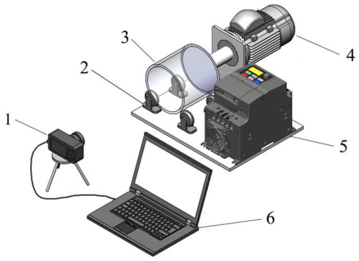
2.1.2. Determination of the Dynamic Angle of Repose

This study adopted a self-made dynamic angle of repose test device (based on the drum method) to measure the dynamic angle of repose, as is shown in Figure 2. The drum was made of organic glass (PMMA). The inner diameter and length were 150 mm and 100 mm, respectively. The material filling rate was 50%. When measuring, the drum was placed horizontally on the bracket wheel and driven by the motor to rotate around its own axis. The motor speed was adjusted by the frequency converter to make the material particles form a smooth flow slope in the drum.

According to the results of the study by Sun et al. [22], the rotation speed of the drum presented a significant impact on the dynamic angle of repose, and the particle swarms in the drum presented different motion characteristics under different rotation speeds, the formula of which can be predicted is as follows:

$$Fr=\frac{{\omega }^{2}R}{g}$$

(1)

where Fr is the Froude number. When 10⁻⁴ < Fr < 10⁻², the motion of particle swarm is rolling; R is the radius of the drum, in m; ω is the rotational angular velocity of the drum, in rad·s⁻¹; and g is the gravity acceleration, in m·s⁻².

Based on the prediction and the preliminary experiment, the drum speed was determined as 6 rpm.

To accurately determine the dynamic angle of repose, a computer image processing technique based on OpenCV was applied to measure the dynamic angle of repose of the particulate materials. The specific process was as follows:

• Use a high-frame-rate camera (resolution ratio: 1280 × 720; frame rate: 120 fps) to capture the flow image of the materials in the drum.
• Apply OpenCV software to denoise the captured image to reduce the impact of noise on the image quality. Detect the edge of the material, extract the boundary and obtain the pixel coordinates of the particle boundary.
• Use the least square method for the fitting of the extracted particle boundary. Calculate the dynamic angle of repose by fitting the linear equation, as shown in Figure 3.

According to the particle size distribution and requirements of the subsequent simulation, we selected the particulate materials with a particle size between 1 mm and 5 mm for a measuring test of the dynamic angle of repose. The test is designed to be repeated 5 times in total. The average dynamic angle of repose was found to be 41.32, with a standard deviation of 1.33.

2.2. Simulated Calibration of Simulation Parameters

2.2.1. Geometric Model

Relevant studies have shown that the shape characteristics of particles have a significant impact on the test results. The contour of the materials indicate that the particles have different shapes and dimensions. Therefore, in order to establish an accurate particle model and to reduce the contour difference between simulated particles and actual particles, a number of staggered stacked spherical particles with different diameters were used to build the geometric models of soil (Figure 4a) and cotton residue (Figure 4b), respectively. To ensure the accuracy of the simulation results and to improve the simulation efficiency, the particle size of the material particle model generated in EDEM was randomly distributed within the range of 0.8~1.2 times the size of the basic particle unit of the non-standard ball, according to the size distribution range measured in the test.

2.2.2. Contact Model

The water content test showed that the particulate materials had a low water content and weak adhesion between the particles. Based on the characteristics and physicochemical property of the material, we adopted the Hertz–Mindlin (no slip) contact model for the discrete element simulation parameter calibration of the particulate materials. This model calculates the motion and force between the particles through the following formula [23,24]:

$$\{\begin{array}{l}{m}_i\frac{d{v}_i}{dt}={\displaystyle \sum _{j=1}^k\left(F_{ij}^{cn}+F_{ij}^{dn}+F_{ij}^{ct}+F_{ij}^{dt}\right)+m_{i}g}\\ I_i\frac{d{\omega }_i}{dt}={\displaystyle \sum _{j=1}^k\left(M_{ij}^t+M_{ij}^r\right)}\end{array}$$

(2)

where m_i is the mass of particle i, in kg; v_i is the translational velocity of particle i, in m∙s⁻¹; ω_i is the angular velocity of particle i, in rad∙s⁻¹; I_i is the rotational inertia of particle i, in kg∙m²; F_ij^cn is the normal contact force between particle i and particle j, in N; F_ij^ct is the tangential contact force between particle i and particle j, in N; F_ij^dn is the normal damping force between particle i and particle j, in N; F_ij^dt is the tangential damping force between particle i and particle j, in N; M_ij^t is the torque between particle i and particle j, in N∙m; M_ij^r is the rolling friction torque between particle i and particle j, in N∙m; and g is the gravity acceleration, in m∙s⁻². The contact force is determined by the shear modulus and Young’s modulus of particles, and the damping force is determined by the collision recovery coefficient, density, shear modulus and Poisson’s ratio of particles. The rolling friction moment is determined by the rolling friction coefficient between the particles.

As the Hertz contact theory regards particles as isotropic materials [25], the particle shear modulus and Young’s elastic modulus can meet the following relationship:

$$G_i=\frac{E_i}{2\left(1+{\mu }_i\right)}$$

(3)

where G_i is the shear modulus of particle i, in Pa; E_i is Young’s modulus of particle i, in Pa; and μ_i is the Poisson’s ratio of particle i.

According to the requirements of the simulation for the parameters, the intrinsic parameters were determined according to the GEMM material library for EDEM software [26,27,28,29]:

• Soil: Poisson’s ratio, 0.4; shear modulus, 1.09 × 10⁶ Pa; density, 1446 kg∙m⁻³;
• Cotton residue: Poisson’s ratio, 0.35; shear modulus, 1 × 10⁶ Pa; density, 319 kg∙m⁻³;
• PMMA: Poisson’s ratio, 0.5; shear modulus, 3.5 × 10⁷ Pa; density, 1180 kg∙m⁻³.

During the simulation, a particle factory was established inside the drum. Then, the particles were dynamically generated and set as virtual. The total mass of particles generated was 2300 g (soil 2064 g and cotton residue 236 g). The mixing ratio of the soil and cotton residue was consistent with the physical test. The generating rate was 100 g/s; the data saving interval was 0.01 s; the fixed time step was 20% of the Rayleigh time step; and the mesh size was three times the minimum spherical cell size. These were compared with the characteristics of the soil and cotton residue of a relevant study [30,31], and the values of the materials were determined with the PMMA simulation contact parameters, as is shown in

Table 2. Table of simulation contact parameter values.

Contact Parameters	Value
Soil PMMA static friction coefficient	0.3
Soil PMMA rolling friction coefficient	0.05
Soil PMMA collision recovery coefficient	0.4
Cotton residue PMMA static friction coefficient	0.45
Cotton residue PMMA rolling friction coefficient	0.1
Cotton residue PMMA collision recovery coefficient	0.3

.

2.2.3. Plackett–Burman Test

Design-Expert software was utilized to perform the Plackett–Burman test design. Then, 9 actual parameters and 2 virtual parameters were selected. For each parameter, 2 levels (high and low) were selected according to relevant research, which were expressed by +1 and −1. A total of 3 central points were selected. A total of 15 tests were conducted, for which the test parameters and levels are shown in

Table 3. The factors and levels table of the Plackett–Burman design.

Parameter Symbols	Parameters	Parameter Levels
		−1	0	+1
T1	Coefficient of recovery friction between soil and soil	0.2	0.3	0.4
T2	Coefficient of static friction between soil and soil	0.2	0.25	0.3
T3	Coefficient of rolling friction between soil and soil	0.05	0.075	0.1
T4	Coefficient of recovery friction between cotton residue and cotton residue	0.4	0.45	0.5
T5	Coefficient of static friction between cotton residue and cotton residue	0.35	0.4	0.45
T6	Coefficient of rolling friction between cotton residue and cotton residue	0.1	0.125	0.15
T7	Coefficient of recovery friction between soil and cotton residue	0.3	0.4	0.5
T8	Coefficient of static friction between soil and cotton residue	0.4	0.5	0.6
T9	Coefficient of rolling friction between soil and cotton residue	0.1	0.15	0.2
T10, T11	Virtual parameters	——	——	——

.

2.2.4. Steepest Climbing Test

The steepest climbing test can effectively obtain the range of the optimal significance parameters. Based on the Plackett–Burman test results, the significant parameters were set to rise with the selected step length, while other non-significant parameters used the middle value of the Plackett–Burman test to conduct the steepest climbing test. The relative error between the simulated dynamic angle of repose and the actual dynamic angle of repose were calculated until the relative error reached the minimum value and then increased gradually. The test scheme and results are shown in

Table 4. Design and results of steepest climbing test.

Test Serial Number	Parameters			Dynamic Angle of Repose σ/(°)	Relative Error ε/(%)
	T2	T3	T5
1	0.1	0.05	0.1	27.72	32.91%
2	0.2	0.10	0.2	36.35	12.03%
3	0.3	0.15	0.3	42.25	2.25%
4	0.4	0.20	0.4	45.88	11.04%
5	0.5	0.25	0.5	48.92	18.39%

. The relative error was calculated by the following formula:

$$\epsilon =\frac{\left|\sigma -\theta \right|}{\theta }\times 100\%$$

(4)

where ε is the relative error; σ is the dynamic angle of repose obtained by simulation test, in °; and θ is the dynamic angle of repose obtained by physical test, 41.32°.

2.2.5. Box–Behnken Test

According to the results of the steepest climbing test, the Box–Behnken response surface test was designed [32,33]. Two levels of each of three significant factors were selected. Five central points were selected for error estimation. A total of 17 tests were performed. The test factor level values are shown in

Table 5. Box–Behnken design test factor level value and coding table.

Code	Coefficient of Static Friction between Soil and Soil (T2)	Coefficient of Rolling Friction between Soil and Soil (T3)	Coefficient of Static Friction between Cotton Residue and Cotton Residue (T5)
+1	0.3	0.05	0.35
0	0.4	0.10	0.4
−1	0.5	0.15	0.45

.

3. Results and Discussion

3.1. Analysis of Plackett–Burman Test Factor Significance

The Plackett–Burman test design used, and the results are shown in

Table 6. Results of Plackett–Burman test.

Test Serial Number	Parameter Notations											Results of Simulation Tests σ/(°)
	T1	T2	T3	T4	T5	T6	T7	T8	T9	T10	T11
1	+1	+1	−1	+1	+1	+1	−1	−1	−1	+1	−1	36.02
2	−1	+1	+1	−1	+1	+1	+1	−1	−1	−1	+1	40.61
3	+1	−1	+1	+1	−1	+1	+1	+1	−1	−1	−1	36.74
4	−1	+1	−1	+1	+1	−1	+1	+1	+1	−1	−1	36.14
5	−1	−1	+1	−1	+1	+1	−1	+1	+1	+1	−1	36.18
6	−1	−1	−1	+1	−1	+1	+1	−1	+1	+1	+1	36.27
7	+1	−1	−1	−1	+1	−1	+1	+1	−1	+1	+1	33.16
8	+1	+1	−1	−1	−1	+1	−1	+1	+1	−1	+1	37.07
9	+1	+1	+1	−1	−1	−1	+1	−1	+1	+1	−1	40.13
10	−1	+1	+1	+1	−1	−1	−1	+1	−1	+1	+1	39.72
11	+1	−1	+1	+1	+1	−1	−1	−1	+1	−1	+1	36.25
12	−1	−1	−1	−1	−1	−1	−1	−1	−1	−1	−1	33.61
13	0	0	0	0	0	0	0	0	0	0	0	37.73
14	0	0	0	0	0	0	0	0	0	0	0	41.36
15	0	0	0	0	0	0	0	0	0	0	0	38.05

. A variance analysis of the results was conducted using Design-Expert software. The influencing effects of each parameter are shown in

Table 7. Analysis of Plackett–Burman test results.

Parameters	Standardized Effects	Sum of Mean Squares	Contribution Degree (%)	Significance Ranking
T1	−0.53	0.83	1.05	7
T2	2.91	25.46	32.00	1
T3	2.89	25.11	31.57	2
T4	0.063	0.012	0.015	9
T5	−0.86	2.24	2.81	3
T6	0.65	1.25	1.58	5
T7	0.70	1.47	1.85	4
T8	−0.65	1.25	1.58	6
T9	0.36	0.40	0.50	8

. As shown, the influencing effects of each parameter on the dynamic angle of repose were, in descending order, as per the following: T₂ > T₃ > T₅ > T₇ > T₆ > T₈ > T₁ > T₉ > T₄. For the convenience of follow-up tests, only the first three parameters that have significant effect were considered, i.e., the coefficient of the static friction between soil and soil (T₂), the coefficient of the rolling friction between soil and soil (T₃) and the coefficient of the static friction between cotton residue and cotton residue (T₅). T₂ and T₃ were positively correlated with the dynamic angle of repose σ, while T₅ was negatively correlated with σ. The main reason is as follows: soil particles have good flowing characteristics and have high proportion in particulate materials. T₂ and T₃ are the major parameters influencing σ. Therefore, they have significant impact on σ; in contrast, the cotton residual material has low mobility when compared with particulate materials, which hindered the particle flow during the dynamic angle of repose test of the particulate materials. As such, T₅ was negatively correlated with σ.

3.2. Analysis of Steepest Climbing Test Results

Table 4 presents the design and results of the steepest climbing test. As shown, the dynamic angle of repose σ gradually increased as T₂, T₃, and T₅ increased, which is consistent with the results of Jiang et al. [26]. The relative error between the σ of the particulate materials obtained by the simulation test and that which was obtained by the physical test, first decreased and then increased. The minimum value was at Level 3, which indicated that the optimal range was around Level 3, and thus we chose this as the central point. Based on the above results, the factors and levels of the Box–Behnken test were deter-mined, as is shown in

Table 8. Box–Behnken design test factor level value and coding table.

Code	Coefficient of Static Friction between Soil and Soil (T2)	Coefficient of Rolling Friction between Soil and Soil (T3)	Coefficient of Static Friction between Cotton Residue and Cotton Residue (T5)
+1	0.3	0.05	0.35
0	0.4	0.10	0.4
−1	0.5	0.15	0.45

.

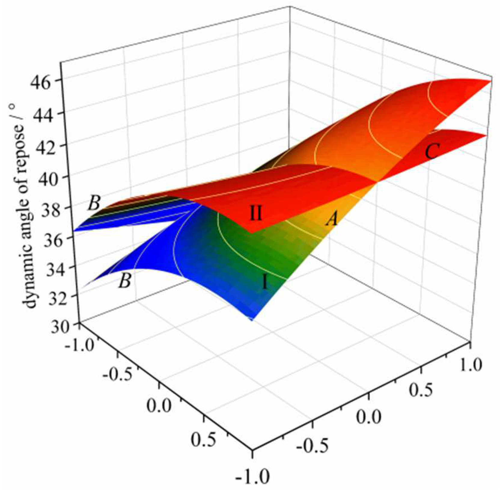
3.3. Analysis of Box–Behnken Test Results

The design and results of the response surface test are shown in

Table 9. Design and results of Box–Behnken test.

Test Serial Number	T2	T3	T5	Dynamic Angle of Repose σ/(°)
1	−1	−1	0	31.7
2	+1	−1	0	34.8
3	−1	+1	0	38.33
4	+1	+1	0	47.46
5	−1	0	−1	38.25
6	+1	0	−1	44.18
7	−1	0	+1	36.61
8	+1	0	+1	42.35
9	0	−1	−1	36.63
10	0	+1	−1	43.27
11	0	−1	+1	34.38
12	0	+1	+1	43.21
13	0	0	0	40.08
14	0	0	0	42.05
15	0	0	0	41.65
16	0	0	0	40.31
17	0	0	0	41.16

. A mathematical model between the dynamic angle of repose σ and the three significance parameters were established using Design-Expert software, as is shown in Equation (5):

$$\sigma =41.05+2.96T_2+4.32T_3-0.72T_5+1.46T_2{T}_3-0.047T_2{T}_5+1.05T_3{T}_5-0.78T_2{}^2-2.25T_3{}^2+0.074T_5{}^2$$

(5)

The results of the regression model variance analysis are shown in

Table 10. ANOVA of the quadratic polynomial model.

Source of Variance	Sum of Squares	Degree of Freedom	Mean Square	F-Value	p-Value
Model	261.34	9	29.04	43.40	¢0.0001 **
T2	70.21	1	70.21	104.95	¢0.0001 **
T3	149.30	1	149.30	223.17	¢0.0001 **
T5	4.18	1	4.18	6.24	0.0411 *
T2T3	8.50	1	8.50	12.70	0.0092 **
T2T5	9.025 × 10−3	1	9.025 × 10−3	0.013	0.9108
T3T5	4.39	1	4.39	6.56	0.0375 *
T22	2.54	1	2.54	3.79	0.0925
T32	21.34	1	21.34	31.90	0.0008 **
T52	0.023	1	0.023	0.034	0.8585
Residual	4.68	7	0.67
Lack of fit	1.82	3	0.61	0.85	0.5348 Not significant
Pure error	2.86	4	0.72
Total	266.02	16
R2 = 0.9824; R2adj = 0.9598; CV = 2.06%

Note: * and ** indicated significance at 0.05 and 0.01 levels, respectively.

. According to Table 10, the simulation test of the dynamic angle of repose σ of the particulate materials and the regression variance analysis showed that T₂, T₃, T₂T₃, and T₃² were the most significant influencing factors of σ; T₅ and T₃T₅ were the significant influencing factors of σ; and other factors were non-significant factors. The influence order of the factors is: T₃ > T₂ > T₃² > T₂T₃ > T₃T₅ > T₅. In the regression variance analysis, the model coefficient p < 0.0001, thus indicating that the relationship between the dependent variables and all the independent variables of the model was extremely significant. In addition, the determination coefficient R² = 0.9824 and the calibration determination coefficient R²_adj = 0.9598 were both close to 1. The variable coefficient was CV = 2.06%. These results indicated that T₂, T₃ and T₅ have a high degree of explanation on the response indicator of σ, and that the quadratic response model has a high reliability.

The influence of the factors on the test indicator can be intuitively analyzed via the response surface chart. Therefore, the response surface chart between T₂, T₃ and T₅ with the dynamic angle of repose σ was made according to the quadratic regression model, and the shape of the response surface could reflect the influence of the interaction items.

In Figure 5, I is the influence surface chart of the interactive item T₂T₃ to the σ of the particulate materials. As is shown, when T₂ and T₃ increased from a low level (−1) to a high level (+1), σ would continue to rise. Compared with T₂, T₃ had a larger impact on σ. Under the interactive effect of T₂ and T₃, σ increased significantly with the increase in the level of the two factors. Further, II is the influence surface chart of the interactive item T₃T₅ to the σ of the particulate materials. When T₃ increased from a low level (−1) to a high level (+1), σ presented an evident increasing trend. Compared with T₂, T₃ had a larger impact on σ. In contrast, when increased from a low level (−1) to a high level (+1), σ presented a slow increasing trend. The corresponding surfaces indicated that T₃ had larger impact on σ than T₅, which is consistent with the result of the variance analysis.

4. Parameter Optimization and Verification Test

4.1. Determination of Optimal Parameter Combination

The optimization module of Design-Expert was adopted for the optimization and solution of the constructed quadratic regression response model, using σ = (41.32 ± 1.33)° as the target value. The results showed that the obtained optimization parameter combination was not the only solution, but also one of a set of several parameter combinations [34,35]. The dynamic angle of repose was simulated by using these optimal solutions, and the combination that was closest to the measured data was selected as the optimal solution, i.e., the coefficient of the static friction between soil and soil, 0.38; the coefficient of the rolling friction between soil and soil, 0.08, and the coefficient of the static friction between cotton residue and cotton residue, 0.33.

4.2. Verification Test

To verify the accuracy of the optimization result, a verification test was conducted on the optimal parameter combination. The significant parameters were determined according to the optimal solution, and the other non-significant parameters were determined according to relevant papers and experiments.

Figure 6 shows the comparison between the simulation test results and physical test results of the dynamic angle of repose under the optimal parameter combination. The mean value of the dynamic angle of repose of the particulate materials after repeated simulation tests was 40.23°. The standard deviation was 1.09°, and the relative error to the value of the physical test was 2.64% (i.e., the dynamic angle of repose obtained by the physical test was the standard value). These results showed that the model has a high reliability.

5. Conclusions

This study adopted the self-made dynamic angle of repose measurement test bench to determine the dynamic angle of repose of the particulate materials in residual film mixture after sieving in cotton field. Based on a physical test, the discrete element simulation tests were carried out using EDEM, and the relevant contact parameters were calibrated by using a Hertz–Mindlin (no slip) contact model.

A Plackett–Burman design test was conducted to screen out the factors that have significant influence on the dynamic angle of repose σ. These factors include the coefficient of the static friction between soil and soil, the coefficient of the rolling friction between soil and soil and the coefficient of the static friction between cotton residue and cotton residue. A steepest climbing test was performed to obtain the level range of the values of the factors. A Box–Behnken test was designed to establish the regression model of the test factors and the dynamic angle of repose. The variance analysis of the regression model showed that the interactive item between the coefficient of the static friction between soil and soil, the coefficient of the rolling friction between soil and soil and the quadratic item of the coefficient of the rolling friction between soil and soil presented a considerably significant impact on the dynamic angle of repose σ. In addition, the coefficient of the static friction between cotton residue and cotton residue, the interactive item between the coefficient of the rolling friction between soil and soil and the coefficient of the static friction between cotton residue and cotton residue presented a significant impact on σ. Moreover, the p-value of other factors was larger than 0.05. Hence, they were non-significant factors to σ. For the established quadratic response model, the coefficient p < 0.0001, the determination coefficient R² = 0.9824, the corrected determination coefficient R²_adj = 0.9598 and the variable coefficient CV = 2.06%. Indicated that the quadratic response model has a high degree of explanation and fitting responsivity, which can accurately predict the dynamic angle of repose σ.

Based on the optimization and solution of the regression equation with σ (obtained through a physical test) as the target value, the following combination of parameters was achieved: static friction coefficient between soil and soil, 0.38; rolling friction coefficient between soil and soil, 0.08; and static friction coefficient between cotton residue and cotton residue, 0.33. A verification test was also conducted on this parameter combination. Results showed that the relative error between the simulation test and physical test was 2.64%, which indicated that the established model was reliable.

References

1. Zhang, H.; Lin, T.; Tang, Q.; Cui, J.; Guo, R.; Wang, L.; Zheng, Z. Effects of planting pattern on canopy light utilization and yield formation in machine-harvested cotton field. Trans. Chin. Soc. Agric. Eng. 2021, 37, 54–63. [Google Scholar]
2. Wang, Z.; He, H.; Zheng, X.; Zhang, J.; Li, W. Effect of cotton stalk returning to fields on residual film distribution in cotton fields under mulched drip irrigation in typical oasis area in Xinjiang. Trans. Chin. Soc. Agric. Eng. 2018, 34, 120–127. [Google Scholar]
3. Hu, C.; Wang, X.; Chen, X.; Tang, X.; Zhao, Y.; Yan, C. Current situation and control strategies of residual film pollution in Xinjiang. Trans. Chin. Soc. Agric. Eng. 2019, 35, 223–234. [Google Scholar]
4. Zhao, Y.; Chen, X.; Wen, H.; Zheng, X.; Niu, Q.; Kang, J. Research status and prospect of control technology for residual plastic film pollution in farmland. Trans. Chin. Soc. Agric. Machin. 2017, 48, 1–14. [Google Scholar]
5. Liang, R.; Chen, X.; Zhang, B.; Meng, H.; Jiang, P.; Peng, X.; Kan, Z.; Li, W. Problems and countermeasures of recycling methods and resource reuse of residual film in cotton fields of Xinjiang. Trans. Chin. Soc. Agric. Eng. 2019, 35, 1–13. [Google Scholar]
6. Jiang, D.; Chen, X.; Yan, L.; Zhang, R.; Wang, Z.; Wang, M. Research on technology and equipment for utilization of residual film in farmland. Trans. Chin. Soc. Agric. Machin. 2021, 41, 179–190. [Google Scholar]
7. Zeng, Z.; Ma, X.; Cao, X.; Li, Z.; Wang, X. Critical review of applications of discrete element method in agricultural engineering. Trans. Chin. Soc. Agric. Machin. 2021, 52, 1–20. [Google Scholar]
8. Marshall, J.S. Discrete-element modeling of particulate aerosol flows. J. Comput. Phys. 2009, 228, 1541–1561. [Google Scholar] [CrossRef]
9. Lorenzo, V.G.; Antonio, B.; Marco, V.; Graziano, F. Micromechanics and strength of agglomerates produced by spray drying. JCIS Open 2023, 9, 100068. [Google Scholar] [CrossRef]
10. Wang, G. Discrete Element Method and Its Practice in EDEM; Northwest University of Technology Press: Xi’an, China, 2010; pp. 15–32. [Google Scholar]
11. Hu, G. Analysis and Simulation of Particle System by Discrete Element Method; Wuhan University of Technology Press: Wuhan, China, 2010; pp. 7–15. [Google Scholar]
12. Li, J.; Tong, J.; Hu, B.; Wang, H.; Mao, C.; Ma, Y. Calibration of parameters of interaction between clayey black soil with different moisture content and soil-engaging component in northeast China. Trans. Chin. Soc. Agric. Eng. 2019, 35, 130–140. [Google Scholar]
13. Wang, X.; Hu, H.; Wang, Q.; Li, H.; He, J.; Chen, W. Calibration method of soil contact characteristic parameters based on DEM theory. Trans. Chin. Soc. Agric. Machin. 2017, 48, 78–85. [Google Scholar]
14. Xiang, W.; Wu, M.; Lu, J.; Quan, W.; Ma, L.; Liu, J. Calibration of simulation physical parameters of clay loam based on soil accumulation test. Trans. Chin. Soc. Agric. Eng. 2019, 35, 116–123. [Google Scholar]
15. Shi, L.; Zhao, W.; Sun, W. Parameter calibration of soil particles contact model of farmland soil in northwest arid region based on discrete element method. Trans. Chin. Soc. Agric. Eng. 2017, 33, 181–187. [Google Scholar]
16. Zhang, R.; Han, D.; Ji, Q.; He, Y.; Li, J. Calibration methods of sandy soil parameters in simulation of discrete element method. Trans. Chin. Soc. Agric. Machin. 2017, 48, 49–56. [Google Scholar]
17. Kanakabandi, C.K.; Goswami, T.K. Determination of properties of black pepper to use in discrete element modeling. Int. J. Food Eng. 2019, 246, 111–118. [Google Scholar] [CrossRef]
18. Cunha, R.N.; Santos, K.G.; Lima, R.N.; Duarte, C.R.; Barrozo, M. Repose angle of monoparticles and binary mixture: An experimental and simulation study. Powder Technol. 2016, 303, 203–211. [Google Scholar] [CrossRef]
19. Hao, J.; Long, S.; Li, J.; Ma, Z.; Zhao, X.; Zhao, J.; Li, H. Effect of granular ruler in discrete element model of sandy loam fluidity in Ma yam planting field. Trans. Chin. Soc. Agric. Eng. 2020, 36, 56–64. [Google Scholar]
20. Geng, L.; Zuo, J.; Lu, F.; Jin, X.; Sun, C.; Ji, J. Calibration and experimental validation of contact parameters for oat seeds for discrete element method simulations. Appl. Eng. Agric. 2021, 37, 605–614. [Google Scholar] [CrossRef]
21. Wang, L.; Fan, S.; Cheng, H.; Meng, H.; Shen, Y.; Wang, J.; Zhou, H. Calibration of contact parameters for pig manure based on EDEM. Trans. Chin. Soc. Agric. Eng. 2020, 36, 95–102. [Google Scholar]
22. Sun, S. Simulation on the Repose Angle of Granular Materials Using Discrete Element Method. Master’s thesis, Hunan University, Changsha, China, 2020. [Google Scholar]
23. Di Renzo, A.; Di Maio, F. Comparison of contact-force models for the simulation of collisions in DEM-based granular flow codes. Chem. Eng. Sci. 2004, 59, 525–541. [Google Scholar] [CrossRef]
24. Malone, K.F.; Xu, B.H. Determination of contact parameters for discrete element method simulations of granular systems. Particuology 2008, 6, 521–528. [Google Scholar] [CrossRef]
25. Johnson, K.L. Contact Mechanics; Cambridge University Press: Cambridge, UK, 1985; pp. 96–119. [Google Scholar]
26. Jiang, D.; Chen, X.; Yan, L.; Mo, Y.; Yang, S. Design and experiment on spiral impurity cleaning device for profile modeling residual plastic film collector. Trans. Chin. Soc. Agric. Machin. 2019, 50, 137–145. [Google Scholar]
27. Feng, D.; Zhao, J. Anatomical structure and basic density of Gossypium Hirsutum stalks. J. Northwest Forest. Univ. 2010, 25, 160–162. [Google Scholar]
28. Feng, X.; Wang, L.; An, Z.; Hu, F.; Xu, G. Correlations between shearing force and nutrient contents of cotton stem. Chin. J. Anim. Nutr. 2016, 28, 3585–3589. [Google Scholar]
29. Zhang, T.; Liu, F.; Zhao, M.; Liu, Y.; Li, F.; Ma, Q.; Zhang, Y.; Zhou, P. Measurement of physical parameters of contact between soybean seed and seed metering device and discrete element simulation calibration. J. China Agric. Univ. 2017, 22, 86–92. [Google Scholar]
30. Ucgul, M.; Fielke, J.; Saunders, C. Three-dimensional discrete element modelling of tillage: Determination of a suitable contact model and parameters for a cohesionless soil. Biosyst. Eng. 2014, 121, 105–117. [Google Scholar] [CrossRef]
31. Tian, Y.; Yao, Z.; Ouyang, S.; Zhao, L.; Meng, H.; Hou, S. Physical and chemical characterization of biomass crushed straw. Trans. Chin. Soc. Agric. Machin. 2011, 42, 124–128. [Google Scholar]
32. Reng, L. Experimental Design and Optimisation, 2nd ed.; Science Press: Beijing, China, 2015; pp. 246–265. [Google Scholar]
33. Douglas, C.M. Design and Analysis of Experiments, 6th ed.; Posts & Telecom Press: Beijing, China, 2009; pp. 354–372. [Google Scholar]
34. Jia, H.; Deng, J.; Deng, Y.; Chen, T.; Wang, G.; Sun, Z.; Guo, H. Contact parameter analysis and calibration in discrete element simulation of rice straw. Int. J. Agric. Biol. Eng. 2021, 14, 72–81. [Google Scholar] [CrossRef]
35. Bai, S.; Yang, Q.; Niu, K.; Zhao, B.; Zhou, L.; Yuan, Y. Discrete element-based optimization parameters of an experimental corn silage crushing and throwing device. Trans. ASABE 2021, 64, 1019–1026. [Google Scholar] [CrossRef]
Figure 1. Particulate materials in residual film mixture after sieving.
Agriculture 13 00959 g001
Figure 2. The dynamic angle of repose test device. 1, high-frame-rate camera; 2, bracket wheel; 3, drum; 4, motor; 5, frequency converter; 6, computer.
Agriculture 13 00959 g002
Figure 3. The dynamic angle of repose measurement. Note: fit the linear equation based on the least square method: y = a0 + a1x; the coefficient of the linear equation: a0, a1; the dynamic angle of repose: σ = arctan(a1).
Agriculture 13 00959 g003
Figure 4. Particle filling model. (a) Soil simulation model; (b) cotton residue simulation model.
Agriculture 13 00959 g004
Figure 5. Surface chart of the influence of interaction items on the dynamic angle of repose. Note: A is the coefficient of the static friction between soil and soil, B is the coefficient of the rolling friction between soil and soil, C is the coefficient of the static friction between cotton residue and cotton residue, I is the interaction between A and B affecting the dynamic angle of repose, II is the interaction between B and C affecting the dynamic angle of repose.
Agriculture 13 00959 g005
Figure 6. Comparison of simulation and physical tests. (a) physical test; (b) simulation test.
Agriculture 13 00959 g006