Insecticide Use by Small-Scale Ugandan Cassava Growers: An Economic Analysis

Abstract

Cassava is the second most important source of calories in Sub-Saharan Africa. It is subject to economically important yield losses from viral diseases, including cassava brown streak disease and cassava mosaic disease. These diseases are vectored by cassava whitefly, so improved approaches for whitefly and disease control are needed to enable smallholder farmers to protect their cassava crops. To investigate the economic viability of insecticide applications against whitefly, the effect of four insecticide application regimes on three cassava genotypes (NASE 3, NASE 12, MKUMBA) and a local landrace were evaluated, for different farmer groups. Data were collected from researcher–farmer managed fields and descriptive statistics were analyzed. Insecticide and personal protective equipment were the major costs for those farmers that applied insecticide and the dipping treatment had a marginal rate of return of 1.66 (166%), demonstrating that this option was the most profitable and effective. While insecticide users incurred more production costs, they also accrued more profit than non-insecticide users, especially if insecticide was applied at early stages of cassava growth. There is a clear need, therefore, to strengthen the commercialization of cassava crop through plant protection measures such as judicious insecticide application on susceptible varieties, so as to increase yield and crop quality.

1. Introduction

Cassava in Uganda is the second most important staple food crop after bananas. It is mostly grown by smallholder farmers and contributes approximately 22% of the total farmer households’ cash incomes [1]. The crop is traded domestically as fresh roots, dry chips, grits and high-quality flour (HQF). It provides 20% of the total national calorie intake with an annual per capita consumption estimated at 119 kg [2]. It is largely grown by 3.9 million smallholder farmers in all regions, in descending order, in the Northern, Eastern, Central and Western regions [3]. The crop is available all year round and contributes to essential nutrients such as carbohydrates, vitamins and minerals [4]. Cassava yields, however, are adversely affected by pests such as whiteflies, mites, thrips and scale insects, which cause significant losses through their feeding damage leading to low cassava productivity (leaves and roots) [5]. The two viral diseases, cassava mosaic disease (CMD) and cassava brown streak disease (CBSD), reduce yields by over 40% (i.e., 42%—CMD; 55%—CBSD) in susceptible varieties [6,7,8].

The African cassava whitefly, Bemisia tabaci SSA1, and its outbreaks are responsible for serious crop yield losses in East and Central Africa resulting in hunger, recurrent famines and annual financial losses of more than US$1.25 billion [9,10,11,12]. Moreover, areas experiencing economically damaging populations of the African cassava whitefly are continuing to expand [13]. Cassava viral disease incidence is increasing rapidly at a time when cassava is becoming a commercial crop and a stimulant for agro-industrial growth in Uganda [4,14,15]. The rapid increase in disease incidence is also associated with the unprecedented increase in the whitefly vector populations [16,17,18,19].

Cassava mosaic disease and CBSD have been managed previously by use of virus-tolerant planting materials with less focus on the whitefly vector [20]. As a way of combating the two viral diseases by targeting the whitefly, researchers at the National Crops Resources Research Institute (NaCRRI), Namulonge, initiated farmer participatory research using insecticides consisting of four treatment regimes (i.e., dipping, early protection, no early protection and no protection) on farmer-managed fields in the districts of Pallisa, Kamuli and Luwero (2019), and Buikwe, Bugiri and Serere (2020). The aim was to evaluate the effectiveness of the protection offered by a widely available systemic insecticide (imidacloprid) in the management of whiteflies for sustainable food security in Sub-Saharan Africa (SSA).

Omongo et al. [21] reported that there were significant root and stem yield differences between chemically treated and non-treated cassava crops. The yields were 40% and 55% lower in non-treated crops for cassava roots and stems, respectively [21]. These yield gaps are a real concern for food security, cassava agro-industrialisation and the seed systems, delivered via cassava seed entrepreneurs. It is because of these yield differences that we were prompted to perform an economic analysis of the different insecticide application treatments, so as to discover the most appropriate recommendations to make to farmers.

To enhance farmers’ adoption, cassava pests and disease control through insecticide applications needs to be cost-effective and practical [22]. This study investigated the economic viability of different insecticide application treatments used by smallholder farmers in Uganda to control whiteflies in cassava crops. To date, there have been several attempts to reduce whitefly populations [23,24,25], but these studies did not include analyses of the costs and benefits involved.

This study therefore, conducted an empirical investigation to address the following research questions: (i) What were the costs and benefits associated with the different levels of insecticide application to control whiteflies in cassava production? (ii) What were the gross margins for the different insecticide application treatments? (iii) Can whitefly-resistant varieties such as MKUMBA be used as an additional control measure to combat super-abundant whitefly populations? (iv) What were the marginal rates of return for the different insecticide application treatments?

2. Materials and Methods

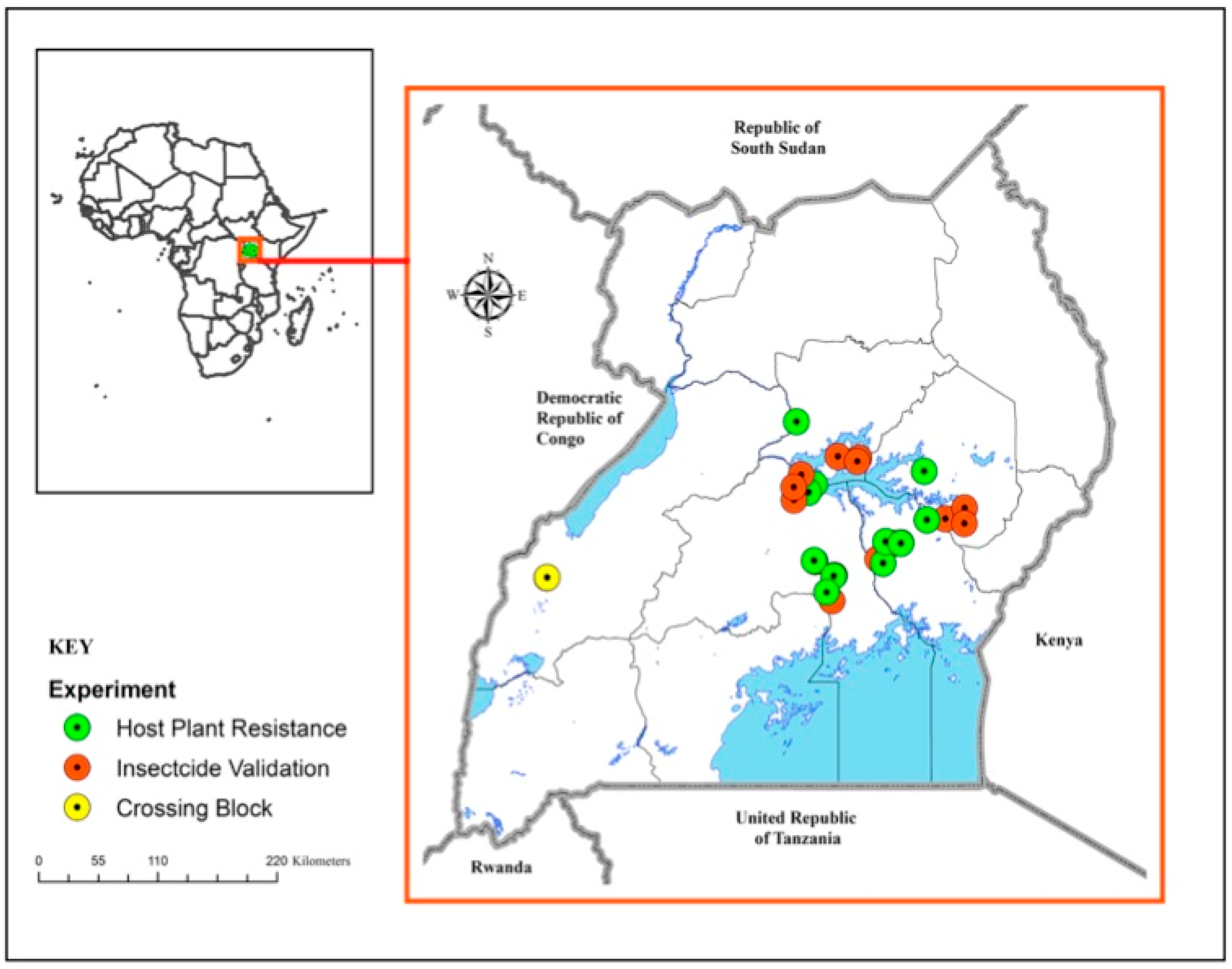
The study was conducted in six cassava-growing districts: Pallisa, Kamuli and Luwero for year one (2019), and Buikwe, Bugiri and Serere for year two (2020) because the cassava whitefly, CMD and CBSD were identified as problems in these districts. Pallisa, Kamuli, Bugiri and Serere are located in the southern Lake Kyoga Plain agroecology in Eastern Uganda, which is drier, while Luwero and Buikwe are in the Lake Victoria Crescent agroecology in Central Uganda which is wetter and more humid (Figure 1).

The trials consisted of five application treatments of imidacloprid insecticide for each cassava variety. Imidacrorid insecticide was used because it is a common, affordable and recommended systemic insecticide in the Ugandan market that is being used to control sucking insects on food crops, orchards, ornamentals, cotton and other crops in the country. This paper will provide the first well-researched evidence for its successful use in cassava to control whiteflies. The treatments were as follows: (i) DP/dipping = no spraying at all but the cuttings are dipped in chemical for some hours before planting (ii) EP/early protection = dipping plus spraying once every 2 months up to 4 months after planting (iii) NEP/no early protection = no dipping but insecticide was applied at 5 and 7 MAP months after planting (iv) NP/no protection = no chemical application at all (v) LP/long protection which consisted of dipping, spraying at 2, 4 and 6 MAP. Prior to planting, cassava cuttings measuring 0.5 m under DP, EP and LP treatments were stacked upright in a plastic basin and drenched in a diluted solution of imidacloprid 200 SL at 3 mls/L for 5 days. Cuttings planted in the “no protection” (control) plots were drenched in tap water to balance any effect in terms of sprouting of the cuttings because of immersion in liquid. After planting, foliar application of imidacloprid 200 SL was carried out using different spray regimes to vary the length (duration) of protection.

This study is the first of its kind in Uganda to critically investigate the timed application of insecticide to control whitefly in cassava. The choice of application intervals was our well-thought-out decision based on the findings of earlier research on whitefly population dynamics which showed that population is highest in the first four months of cassava growth. Through its dual role as a vector and a pest, this is also the period in which whitefly causes high feeding damage and spread of the viral diseases. This study will therefore provide the first recommendation of the spraying intervals/period which is economical to effectively control whitefly in cassava. Spraying was only carried out when there was little or no wind in order to avoid drift. The foliar treatments were carried out using a CP15 backpack knapsack sprayer (15 L-capacity) with a hydraulic cone nozzle. The dosage of imidacloprid 200 SL used was 30 mls per CP15 backpack in year one. In year two, the LP regime was eliminated, because it was clearly too costly, leaving only four treatment regimes for the experiment.

The cassava genotypes used across trials were: NASE 3, NASE 12 and MKUMBA, plus a local popular check that varied from district to district, which were Kabwa/Matooke/Kalitunsi (Buikwe), Magana or China-0 (Bugiri) and Edyala (Serere). The selection of the 3 varieties was based on their differential response to B. tabaci infestation: MKUMBA is known to be resistant, NASE 3 is tolerant and NASE 12 is susceptible to whitefly infestation. We envisaged that insecticide application by dipping the cuttings prior to planting and spraying during the critical growth stage (1–4 months after planting) would demonstrate the effect and economics of insecticide protection for varieties which are resistant, tolerant and susceptible. NASE 3 and NASE 12 have been commonly grown by farmers since their releases in 1993 and 2001, respectively. Meanwhile, MKUMBA is a recent introduction and proved resistant to whiteflies, hence was a good control treatment for the insecticide application experiment.

Each variety was exposed to all the treatments in separate plots of the same field. In total, there were 20 and 16 plots per field for trial 1 and trial 2, respectively. Each plot consisted of 36 plants. The plot sizes were 5 m by 5 m arranged in a randomized complete block design (RCBD) with a spacing of 1 m by 1 m between cassava plants.

Prior to farmer data collection, the different farmer groups received training on whitefly and the associated damage symptoms. These groups then collected data on the prevalence of whitefly, CMD and CBSD independently, in addition to those experimental data collected by the researchers. The different farmer groups (18 groups) acted as the replicates in the analyses of the farmer-collected data. The researchers collected data from the same farmer-participatory trials and demonstrations to test whether, or not, they generated substantial and clear benefits in terms of farmers’ increased yields and income, as well as significantly reducing cassava whitefly populations and disease incidences.

The effect of the different insecticide regimes was evaluated in the plots at 1, 2, 4, 5, 7 and 12 months after planting (MAP) for whitefly infestation, CBSD foliar symptoms and CMD. At 12 MAP, harvesting was carried out and data were collected from the inner rows of each plot excluding the border rows because of undue agronomic benefits. The average plot size for the inner plot consisted of 16 plants. The severity of CBSD root necrosis was assessed using a scale of 1–5 [26,27,28], where 1 = no apparent root necrosis, 2 = less than 5% of root necrotic, 3 = 5–10% of root necrotic, 4 = 10–25% of root necrotic, mild root constriction and 5 = >25% of root necrotic with severe root constriction.

For CMD, the assessment scale used was, 1 = un-affected shoots, or no symptoms observed, 2 = mild chlorotic pattern on most leaves, mild distortions at the bases of most leaves, while the remaining parts of the leaves and leaflets appear green and healthy, 3 = pronounced mosaic pattern on most leaves, narrowing and distortion of the lower one- third of the leaves, 4 = severe mosaic distortion of two-thirds of most leaves and general reduction in leaf size, and some stunting of shoots, and 5 = very severe mosaic symptoms on all leaves, distortion, twisting and severe leaf reduction in most leaves accompanied by severe stunting of plants [26,29].

2.1. Data Analysis

To determine the economic performance of different treatments, a cost–benefit analysis (CBA) was conducted, as described by Dewri et al. [30] and Weimer [31]. The cost–benefit analysis seeks to place monetary values on both the inputs (costs) and outcomes (benefits) [32].

To achieve this, operations realized were specified in the three stages of production:

• Pre-sowing (ploughing or other tillage, dipping of cuttings and planting)
• Husbandry (insecticide application and weeding)
• Harvest (crop harvest, product sorting and grading)

For each of the alternatives, the type of equipment involved, the labor (man hours), the quantity and type of inputs applied, as well as their open market prices, were specified.

Following Dewri et al. [30], we use the benefit–cost ratio (BCR) together with the marginal rate of returns (MRR) to arrive at the best (most cost effective) treatment. The BCR helps to derive the ratio of whitefly control alternatives’ benefits versus costs, which helps to determine the viability and value that can be derived from an investment. All things being equal, farmers should be willing to accept a treatment if the BCR of that treatment is greater than the minimum acceptable BCR of 1.5 (BCR > 1.5). A treatment with a ratio greater than 1 (BCR > 1) is considered economically viable and BCR =1 is the breakeven point. Nonetheless, due to the cost of capital and inflation the minimum acceptable BCR for an investment to be considered viable is a BCR of 1.5. BCR involves summing up the total discounted benefits for a given alternative over its entire duration, which is one year for cassava, and dividing it by the total discounted costs for that alternative. The advantage of using BCR is that it helps to compare various options in a single term and helps in deciding faster which options should be preferred or rejected. Unlike the net present value (NPV) model which helps to determine whether a treatment should be invested in or not, the BCR model helps to solve the dilemma of choosing between two or more treatments based on the BCR, whereby the one with the highest BCR is chosen as the most worthwhile option [33]. In the process, the gross margins for the different alternatives were also computed. The gross margin is the difference between the gross farm income (total revenue) and the costs incurred during production (total variable cost). The analysis to achieve gross margins was carried out as follows:

$$GM=TR-TVC$$

(1)

where $GM=$ gross margin; $TR=$ total revenue (price × marketable quantity); $TVC=$ total variable cost (i.e., costs which change as output changes).

2.2. Estimates of Costs and Benefits Associated with Cassava Production under Insecticide Control of Whitefly

The estimated costs included costs of equipment, labor and inputs (insecticide, water). The value of labor was captured as per activity/task completed by the farmer group and the cost per hectare of different operations specified. The cost of planting material (cuttings) was not considered because it does not vary with varieties and remains constant in all locations of the study. Indeed, they are considered as farmers’ saved materials in East Africa [34,35] and they did not incur any cost at the time of the study. Fixed costs such as land, buildings (for storing equipment) or insurance were not included. Total costs that vary for each control method were calculated using the following formula, as stated by CIMMYT [36]:

$$C_i=\sum V_i$$

(2)

where $V_i$ represents the costs that vary in Uganda shillings in period i, which includes labor, chemicals and the rental of a sprayer to apply the chemical among others.

The benefits were represented by the saving of cassava from whitefly damage, calculated as the market value of the roots. The yield corresponds to the part of the harvest that can be sold or used for self-consumption. The yield in this experiment was adjusted downwards by 20% to cater for differences in management (10%), plot size (5%) and harvest date (5%) [36]. The output price was the farm gate price as stated by the farmers. The impact of the output price on the profitability of insecticide use was analyzed through sensitivity analysis. The costs and benefits for the period of two seasons, 2019 and 2020, were calculated. The benefit–cost ratio (total benefits divided by total costs) was determined by comparing the costs incurred for chemical control with the financial benefits resulting from the control, i.e., the commercial value of plants that were saved from whitefly infestation. The resulting ratio expressed the efficiency of the treatment for the period considered.

Cost–benefit analysis not only based decisions on costs and benefits, but also examined the value of net benefits (NB), after deducting costs from benefits [37]. The net benefits were computed as the value of benefits gained minus the value of costs incurred. The formula in Equation (3) was employed to calculate the benefit–cost ratio (BCR), i.e., BCR = total cassava benefits/total production cost:

$$BC{R}_i=\frac{\sum B_i}{\sum C_i}$$

(3)

where $B_i$ = the whitefly control alternative’s benefit in year i, where i = 0 to n years ($n$ = the total number of years for the whitefly control alternative’s duration); $C_i$ = the whitefly control alternative’s costs in year i, where i = 0 to n years. Since the costs and benefits for the different treatments were largely constant over the study duration of two years, the benefit cost ratio was computed without discounting.

Table 1. Interpretation of BCR.

BCR < 1.0	BCR = 1.0	BCR > 1.0
In economic terms, the costs exceed the benefits. Solely on this criterion, the whitefly control alternative should not be allowed to proceed.	Costs equal the benefits, which means the whitefly control alternative should be allowed to proceed, but with cautious support.	The benefits exceed the costs, and the whitefly control alternative should be allowed to proceed.

below:

The calculated benefits and costs of a given whitefly control alternative vary depending on the input data applied in the cost–benefit analysis. The range of potential outcomes for differing inputs were gauged using a sensitivity analysis, to determine where the potential net benefits of whitefly control alternative would be negative.

2.3. Calculation of the Marginal Rates of Return for the Different Spray Regimes

The marginal rate of return was estimated as the amount of revenue per additional item, divided by the cost per additional item produced. In other words, it is the amount of additional revenue that a cassava farmer would expect to earn for each additional shilling that she/he spends on production. Using a marginal rate of return, a farm can determine whether, or not, the operations are profitable. According to CIMMYT [36] and Varian [38], the easiest way to describe feasible production plans is to list them: that is, listing all combinations of inputs and outputs that are technologically feasible. The set of all combinations of inputs and outputs that comprise a technologically feasible way to produce is called a production set.

Goto and Suzuki [39] and Nicholson and Snyder [40] proposed a Cobb–Douglas production function of the form in Equation (4):

$$f\left(x_1,x_2\right)=Q_i=\alpha x_1^a{x}_2^b$$

(4)

where $Q_i$ is the quantity of cassava harvested from a given plot/spray option i, $x_1$ and $x_2$ are the inputs used in cassava whitefly control, the parameter $\alpha$ measures the scale of production (how much output would be obtained if one unit of each input was used). The parameters a and b measure how the amount of output responds to changes in the inputs $x_1$ and $x_2$, respectively. In log-linear models, Equation (5) becomes:

$$\ln q=\ln A+a\ln x_1+b\ln x_2.$$

(5)

Coefficient A (originally $\alpha$) represents the percent increase in $Q_i$ (taking the log of its values) for a 1 unit increase in $x_i$ (not log transformed):

$$\alpha =\frac{\Delta \ln \left(Q\right)}{\Delta x}$$

(6)

Hence, A is an estimate for the rate of return for an added input unit, $\alpha$ ≈ MRR. Thus, the marginal rate of returns was estimated as the increase in net benefits for each additional insecticide spray divided by the additional spray costs, i.e., $MRR=\frac{\mathrm{increase} \mathrm{in} \mathrm{net} \mathrm{benefits}}{\mathrm{additional} \mathrm{spray} \mathrm{costs}}\times 100$.

To determine the most acceptable recommendation, the different insecticides application treatments were arranged in order of increasing costs. Comparisons were made between one alternative and the next in a stepwise manner. A value of marginal rate of return of less than one was an indication that the increase in cassava returns did not compensate for the additional cost of applying insecticide [21,36].

2.4. Cost Efficiency Analysis

To generate profit, resources are used to produce some level of output which could positively influence production cost. To examine this relationship, a stochastic frontier cost analysis [41,42] was performed on 18 farmer groups with about 200 farmers in total. The cost function approach was preferred over the profit function approach to avoid problems of estimation that may arise in situations where farm households realize zero or negative profits at the prevailing market prices [41,43]. The model helps to account for the inefficiency component separately from measurement error and other statistical noise in the data. Accordingly, a stochastic cost function was constructed using a Cobb–Douglas function form (Equation (7))

$$\ln C={\beta }_0+{\displaystyle \sum }_{i=1}^3{\beta }_i\ln P_i+{\beta }_4\ln Q+V_i+U_i$$

(7)

where:

C = minimum cost associated with cassava production

P_i = price of variable input (insecticide, personal protective equipment, labour to apply insecticide)

Q = cassava output measured in kg

β_i = vector of parameters

V_i = random variables such that Vi is normally distributed with a mean of 0 and variance σ²_v.

U_i = non-negative random variables that account for cost inefficiency such that Ui are independently distributed with a mean µ variance σ²_u.

3. Results and Discussion

3.1. Summary Statistics on Cassava Production

The average number of plants harvested per plot was 11, although NASE 12 had a higher number at 13 plants (

Table 2. Cassava Production summaries by variety.

Variety	No. of Plants/Plot	Total Number of Tubers/ha	Total Tuber Weight (kg)/ha	Marketable Tuber Weight (kg)/ha	Farm Gate Price (UGX/kg)
LOCAL	11.61	61,542.58	29,128.42	24,632.13	323.57
MKUMBA	10.46	56,073.94	25,298.68	22,629.07	312.58
NASE 3	10.65	70,271.98	27,091.43	24,491.58	324.93
NASE 12	12.85	83,801.55	30,471.61	26,541.50	336.54
Average	11.39	67,922.51	27,997.54	24,573.57	324.40

Source: Field Data, 2020 and 2021.

). The higher number of plants for NASE 12 was attributed to the high germination percentage and good plant establishment. Generally, improved varieties produced more tubers than the landraces. The tuber yield per hectare was highest with NASE 12 at 83,802 tubers followed by NASE 3 at 70,272. The improved cassava varieties had more root weight compared to the landraces. The cassava yield (weight of roots) was greatly influenced by variety cultivated. NASE 12 had the highest marketable weight of 26,542 kg per hectare followed by the local variety with 24,632 kg and then NASE 3 at 24,492 kg. This is consistent with Manze et al. [44], who found that the top performers (in terms of high yield and disease resistance) were mostly the improved varieties released after 2011 while the worst performers were the local varieties. Given the high yielding and pest and disease resistance attributes of improved cassava varieties, there is a need to stimulate the demand for these varieties by relaxing the constraints farmers face when accessing agricultural knowledge and improved varieties.

Cassava farmers stated the farm gate prices per kilogram of NASE 12, NASE 3 and local to be higher than that of MKUMBA (Table 2). Generally, at the farm gate, a farmer expected to get about 324 shillings (Exchange rate: 1 USD = 3600 (average exchange rate for August 2020 to August 2021)) per kilogram of fresh cassava compared to about 576 shillings, if they travelled to the market. Although MKUMBA is resistant to whiteflies, CMD and CBSD [45], and has high dry matter content as well as excellent sensory attributes for flour-based meal, it fetched a lower price than the local variety. This might be attributed to the fact that farmers’ verdicts were based on raw and boiled root assessment with consideration of yield, taste, mealiness and fibrousness, where MKUMBA was rated poorly compared to other varieties. In contrast, NASE 12 fetched the highest price at the farm gate of 336 shillings per kilogram. This shows the need for breeding teams to collaborate with multidisciplinary teams to collect all relevant data to provide additional data points for breeding decisions.

Comparing average prices by location, farmers in Bugiri indicated that they received about 397 shillings per kilogram at the farm. These were followed by Pallisa and the least was Luwero (

Table 3. Average cassava farm gate prices by location.

District	Farm Gate Price (UGX/kg)
Bugiri	396.51
Buikwe	315.39
Kamuli	289.92
Luwero	234.34
Pallisa	360.97
Serere	349.30
Average	324.40

Source: Field Data, 2020 and 2021.

). This could be attributed to the fact that Bugiri, Pallisa and Serere are located in areas of high cassava production and consumption, which generated high demand and therefore better market prices compared to Luwero and Buikwe, where the crop is mainly for home consumption. Luwero had the lowest farm gate price perhaps because the main staple food in Luwero is cooked banana (popularly known as “matooke” in Uganda) and cassava is mainly used locally as snacks. Hence farmers produce and eat more banana than cassava given that the demand for fresh tubers locally is less. Indeed, cassava in Luwero is consumed wholly fresh, hence has a limited utilization base while, in Eastern Uganda, cassava is both for food security and a major source of income [46]. It has high demand both at a domestic level and regional level in Kenya in the form of chips and flour. With this wide utilization base, including industrial use, the price goes up compared to Luwero in Central Uganda that uses bananas as a major source of food and income. This is in line with Nakabonge et al. [46] who found that, in the Teso region (Eastern Uganda), farmers mostly grew improved cassava varieties which were essentially for commercial purposes, hence the high price.

3.2. Costs and Benefits of Insecticide Application to Control Whiteflies in Cassava

With regards to the average costs per hectare, these varied across treatment regimes. For instance, the early protection (EP) costs were approximately 4.1 million shillings/ha followed by NEP at 3.91 million shillings/ha and DP was 3.89 million shillings/ha (

Table 4. Cassava costs and revenue per hectare by treatment regime and variety (‘000).

	Production Costs	Variety				Avearge
		LOCAL	MKUMBA	NASE 12	NASE3
Treatment Regime	Cost (UGX/ha)	Income (UGX/ha)	Income (UGX/ha)	Income (UGX/ha)	Income (UGX/ha)	Revenue (UGX/ha)	Net Benefits (UGX/ha)
DP	3894	11,100	8475	10,500	7976	9509	5615
EP	4095	8965	7585	9410	8897	8714	4620
NEP	3914	7157	5875	9552	6790	7343	3429
NP	2988	6000	8664	7210	8230	7526	4538
Average	3862	8306	7650	9163	7973	8273	4411

NB: DP/dipping = no spraying at all but the cuttings are dipped in chemical for some hours before planting, EP = dipping plus spraying once every 2 months up to 4 months after planting, NEP (no early protection) = no dipping and spraying starts at 5 months after planting for once every 2 months up to 7 months after planting and NP = no chemical application at all. Source: Field Data, 2020 and 2021. (‘000) = figures are in thousands.

). To ensure uniform results, analysis was carried out without the long protection (LP) treatment regime, since it was eliminated after season one.

NASE 12 registered the highest incomes per hectare of 9.2 million shillings/ha followed by the local variety at 8.3 million shillings/ha and the NASE 3 at 8.0 million shillings/ha due to the higher prices attached to them. However, by spray regime, NASE 12 and local varieties brought more income under the DP treatment, while NASE 3 and the MKUMBA brought more income under EP and NP treatments (Table 4). This implies that, while it is encouraged to use imidacloprid at the early stages of cassava growth on whitefly susceptible varieties so as to increase cassava yield (weight of roots) and hence result in higher incomes, it is not cost effective to apply insecticide for whitefly control on whitefly-resistant varieties. Overall, DP was the most worthwhile treatment because it resulted in the net revenue. This is in line with Avicor et al. [47] who stated that farmers should be encouraged regarding the judicious use of insecticides to control cassava whitefly with sustained monitoring of their resistance status to these insecticides.

The farmers in Pallisa, Kamuli and Bugiri earned more income under DP (13.3, 10.3 and 8.4 million shillings/ha, respectively), in Luwero and Serere they earned more under EP (10.9 and 10.8 million shillings/ha, respectively) and in Buikwe they registered more income under NEP with 6.1 million shillings/ha (Appendix A,

Table A1. Costs and revenues by spray regime and district (‘000).

	All Districts	Bugiri	Buikwe	Kamuli	Luwero	Pallisa	Serere
Treatment Regime	Cost (UGX/ha)	Income (UGX/ha)	Income (UGX/ha)	Income (UGX/ha)	Income (UGX/ha)	Income (UGX/ha)	Income (UGX/ha)
DP	3894	8422	5957	10,300	8488	13,300	10,600
EP	4095	6922	4760	8207	10,900	10,600	10,800
NEP	3914	8667	6118	5605	8414	6209	9046
NP	2988	6402	5523	7131	10,500	7045	8589
Average	3862	7603	5589	7799	9573	9295	9779

(‘000) = figures are in thousands.

). An analysis of variance (ANOVA) test on tuber yield was conducted using a one-way ANOVA [48]. Bartlett’s chi-squared statistic rejected the null hypothesis of equal means at the 1% level (

Table 5. Analysis of variance (ANOVA) to compare means of treatment regimes (‘000).

Source	Sum of Square	Degrees of Freedom	Mean Square	F Statistic	Prob > F
Between groups	7,039,500	3	2,346,500	9.05	0.000
Within groups	73,636,000	284	259,280
Total	80,675,000	287	281,098
Treatment Regime	Mean Yield/Ha	Std. Deviation
DP	27.31	17.81
EP	34.22	14.63
NEP	29.88	16.73
NP	20.58	15.03
Average	28.00	16.77

NB: DP/dipping = no spraying at all but the cuttings are dipped in chemical for some hours before planting, EP = dipping plus spraying once every 2 months up to 4 months after planting, NEP (no early protection) = no dipping and spraying starts at 5 months after planting for once every 2 months up to 7 months after planting and NP = no chemical application at all. Source: Field Data, 2020 and 2021. (‘000) = figures are in thousands.

).

3.3. Gross Margins of Different Levels of Insecticide Application to Control Whiteflies

NASE 12 emerged as the most profitable variety, where a farmer has the potential to earn approximately 5.3 million shillings per hectare. This was followed by local and NASE 3 varieties, with gross margins of 4.4 and 4.1 million shillings per hectare, respectively. However, by insecticide application, the DP treatment regime gave high and positive gross margins across varieties including the local ones, followed by the EP treatment regime, while NEP exhibited the lowest profit except under NASE 12 and local varieties as shown in

Table 6. Gross margins (UGX/ha) by variety (‘000).

Treatment Regime	LOCAL	MKUMBA	NASE 12	NASE 3	Average
DP	7206	4581	6606	4082	5615
EP	4870	3490	5315	4802	4619
NEP	3243	1961	5638	2876	3429
NP	3012	5676	4222	5242	4538
Average	4444	3788	5301	4111	4411

NB: DP/dipping = no spraying at all but the cuttings are dipped in chemical for some hours before planting, EP = dipping plus spraying once every 2 months up to 4 months after planting, NEP (no early protection) = no dipping and spraying starts at 5 months after planting for once every 2 months up to 7 months after planting and NP = no chemical application at all. Source: Field Data, 2020. (‘000) = figures are in thousands.

.

The cassava variety MKUMBA registered a gross margin of about 5.7 million shillings per hectare under no protection. This implies that for whitefly resistant varieties, it is not cost effective to apply insecticide for whitefly control. For the susceptible varieties, however, a judicious application of insecticide by dipping, or dipping and spraying once at two and four months of planting, would be sufficient. This is consistent with Legg et al. [49], who proposed the need to strengthen efforts to commercialize cassava crop through plant protection measures in order to have an increased yield and higher standards of crop.

On average, a farmer in Serere earned gross margins of about 5.9 million shillings per hectare while, in Luwero, the margins were 5.7 million shillings per hectare and 5.4, 3.9, 3.7 and 1.7 million shillings per hectare in Pallisa, Kamuli, Bugiri and Buikwe, respectively (

Table 7. Gross margins (UGX/ha) by location (‘000).

Treatment Regime	Bugiri	Buikwe	Kamuli	Luwero	Pallisa	Serere	Average
DP	4528	2063	6406	4594	9406	6706	5617
EP	2827	665	4112	6805	6505	6705	4603
NEP	4753	2204	1691	4500	2295	5132	3429
NP	3414	2535	4143	7512	4057	5601	4544
Average	3741	1727	3937	5711	5433	5917	4411

NB: DP/dipping = no spraying at all but the cuttings are dipped in chemical for some hours before planting, EP = dipping plus spraying once every 2 months up to 4 months after planting, NEP (No early protection) = no dipping and spraying starts at 5 months after planting for once every 2 months up to 7 months after planting and NP = no chemical application at all. Source: Field Data, 2020 and 2021. (‘000) = figures are in thousands.

). The DP and EP regimes still registered high margins per hectare across the districts and NEP exhibited the lowest gross margins except in Buikwe and Bugiri districts. This could be attributed to the low whitefly population and lower disease pressure at the time of the study in Buikwe and Bugiri districts, making it less economical to use insecticide in these areas.

Running gross margin scenarios for the two best performing improved varieties, i.e., NASE 12 and NASE 3, we generated scenarios based on changes in prices and gross margins. Economic theory indicates that, if all things remain constant (ceteris Paribas), a change in price brings about a change in variable costs as well. Hence, as we varied prices/revenues, variable costs also varied. Under the DP treatment regime, NASE 12 was the most profitable when the price hypothetically increased by 25% and costs reduced by 25% leading to a gross margin of 5.2 as indicated in

Table 8. Gross margin scenarios (UGX/ha) for NASE 12 variety (‘000).

Price Increase %	Variable Cost Reduction %	Treatment Regime 1	Gross Margin 1 (UGX)	Treatment Regime 2	Gross Margin 2 (UGX)
10%	10%	DP	2050	EP	1931
15%	15%	DP	3175	EP	2802
20%	20%	DP	4200	EP	3772
25%	25%	DP	5225	EP	4743

NB: DP/dipping = no spraying at all but the cuttings are dipped in chemical for some hours before planting, EP = dipping plus spraying once every 2 months up to 4 months after planting. Source: Field Data, 2020 and 2021. (‘000) = figures are in thousands.

.

NASE 3 was the most profitable when the price changed by 25% and costs changed by 25% leading to a gross margin of about 3.9 and 4.4 million shillings per hectare under the DP and EP treatment regimes, respectively (

Table 9. Gross margin scenarios (UGX/ha) for NASE 3 variety (‘000).

Price Increase %	Variable Cost Reduction %	Treatment Regime 1	Gross Margin 1 (UGX)	Treatment Regime 2	Gross Margin 2
10%	10%	DP	1596	EP	1780
15%	15%	DP	2392	EP	2638
20%	20%	DP	3190	EP	3582
25%	25%	DP	3988	EP	4427

NB: DP/dipping = no spraying at all but the cuttings are dipped in chemical for some hours before planting, EP = dipping plus spraying once every 2 months up to 4 months after planting. Source: Field Data, 2020 and 2021 (‘000) = figures are in thousands.

).

A sensitivity analysis revealed that NASE 12 and NASE 3 gross margins were more sensitive to price changes of 20% and 25% as shown in

Table 10. Sensitivity analysis of gross margins to price and variable cost changes for NASE 12 and NASE 3.

Price Increase %.	Variable Cost Reduction%	Gross Margin Sensitivity Price Changes
10	10	0.18
15	15	0.26
20	20	0.33
25	25	0.40

Source: Field Data, 2020 and 2021.

. Though at these price levels incomes would significantly increase, the high increase in costs would be prohibitive for farmers, hence the 10% and 15% price change would be more favorable. This is in line CIMMYT [36], which states that whether farmers market little or most of their produce, they are interested in the economic return. Farmers will always consider the costs and risks of changing from one practice to another and the economic benefits resulting from that change. Researchers, therefore, should be clear about the benefits, costs and risks associated with a particular technology for farmers to make rational decisions.

3.4. Calculated Benefit–Cost Ratios (BCR) and Analysis of Variance for the Different Treatment Regimes

While all insecticide application regimes had their BCRs above one, DP, EP and NP treatment regimes were above the minimum acceptable BCR of 1.5 (

Table 11. Cassava production costs and yields of different insecticide application treatments.

Item	Treatment Regime (‘000)
	DP	EP	NEP	NP
Bush clearing	173	173	173	173
Ploughing	296	296	296	296
Planting	296	296	296	296
Weeding	1482	1482	1482	1482
Dipping + Spraying labor	108	276	128
Harvesting labor	741	741	741	741
Insecticides
Imidaclopid (Confidor)	35	68	35
Equipment
Gumboots	80	80	80	80
Overcoats	180	180	180
Goggles	40	40	40
Gloves	40	40	40
Jerricans	28	28	28
Drum	80	80	80
Knapsack sprayers	160	160	160
Nose masks	24	24	24
Basins	32	32	32
Soap	99	99	99
Total Cost_ha	3894	4095	3914	3068
Marketable Yield_ha (kg)	26	26	22	23
Adjusted Market Yield_ha (kg) (20%)	21	21	18	19
Farm Gate Price (UGX)	0.354	0.321	0.310	0.313
Gross Benefits_ha (UGX)	7365	6777	5562	5870
NET BENEFITS_Ha (UGX)	3471	2683	1648	2802
BCR = Gross Benefits/Total Cost	1.9	1.7	1.4	1.9

NB: DP/dipping = no spraying at all but the cuttings are dipped in chemical for some hours before planting, EP = dipping plus spraying once every 2 months up to 4 months after planting, NEP (no early protection) = no dipping and spraying starts at 5 months after planting for once every 2 months up to 7 months after planting and NP = no chemical application at all. Source: Field Data, 2020 and 2021.

). However, it is important to note that simply following a rule that a BCR above one indicates success, and that a BCR below one would mean a failure or a rejection decision, can be misleading and may lead to a misfit with the intervention in which heavy investment is made. Hence, the BCR should be used as a conjunctive tool with different types of analysis such as the use of marginal rate of return (MRR) and other qualitative factors to make a good decision [30]. Similarly, Otte et al. [50] observed that a cost–benefit analysis is expected to indicate the management option with the greatest net benefits, but it does not by itself determine the best management choice.

3.5. Marginal Rates of Return for the Different Spray Regimes

Overall, the marginal rate of return on moving from NP to DP was 1.66 (166%) and it was above 100% which is the minimum acceptable rate of return [36], as shown in

Table 12. Marginal rate of returns for the lowest cost treatment regime.

Treatment	Total Costs That Vary (Shs/ha) (‘000)	Net Benefits (Shs/ha) (‘000)	Marginal Rate of Return
NP	3068	2802	-
DP	3894	3471	1.66 (166%)
NEP	3914	1648	−91.15 (−9115%)
EP	4095	2683	−3.93 (−393%)

NB: DP/dipping = no spraying at all but the cuttings are dipped in chemical for some hours before planting, EP = dipping plus spraying once every 2 months up to 4 months after planting, NEP (no early protection) = no dipping and spraying starts at 5 months after planting for once every 2 months up to 7 months after planting and NP = no chemical application at all. Source: Field Data, 2020 and 2021. (‘000) = figures are in thousands.

. The yields of treatment regime EP were higher than those of treatment regime NP, but the value of the increase in yield was not enough to compensate for the increase in costs. Therefore, DP was certainly the most worthwhile alternative to the farmers’ practice of no protection. Treatment regimes EP and NEP had higher costs but fewer net benefits than NP, hence EP and NEP were dominated treatment regimes [32]. The DP treatment regime registered the highest yield and its costs provided an acceptable rate of return. The regime is less costly in terms of the quantity of chemicals and other associated expenses. Since cassava is protected during the critical growth period of 1–2 months after planting [51], there is less disease incidence and less farmer exposure to chemical contact. Furthermore, applying chemicals to cassava cuttings at planting saves on time spent on insecticide spraying activities. Thus, while all treatment regimes registered positive net benefits, these were highest for the DP treatment. Therefore, the judicious application of systemic insecticide at planting provided the most cost effective control of whitefly problems in cassava production and improved root yield hence resulted in higher returns. This suggests that, for farmers to maximize their cassava returns, they should not apply insecticide beyond dipping.

3.6. Estimated Cost Function

The results obtained through marginal analysis confirmed that the judicious use of insecticides at the planting of cassava was the most cost effective treatment as it yielded more returns on investment. Further analysis was performed to determine whether resources were being used efficiently (cost minimization) given the current level of output. The estimates of the stochastic frontier cost function are as indicated in

Table 13. Stochastic cost frontier for cassava production.

Stoc. Frontier	Normal/Truncated-Normal Model	Number of Obs = 178
Log likelihood	405.84142	Wald chi2(4) = 2535.04
Variable		Prob > chi2 = 0.000
lnTotalCOST_ha	Coefficient	Standard Error
Chemical price	1.4 × 10−6 ***	2.6 × 10−7
PPE price	4.6 × 10−7 ***	2.7 × 10−8
Labor on chemical use price	3.9 × 10−7	3.5 × 10−7
lnOutput_ha	1.3 × 10−4	1.4 × 10−3
Constant	1.5 × 10 ***	1.4 × 10−2
sigma2	6. × 10−3	2.1 × 10−3
gamma	9.8 × 10−1
sigma_u2	5.9 × 10−3
sigma_v2	9.9 × 10−5

***: Significant at 1% level, ln = log transformation. Source: Field Data, 2020 and 2021.

. The coefficient of chemical application price had a significant and positive relationship with the cost of cassava production. This implies that chemicals were a significant cost in cassava production in the study area. This suggests that any policy to increase cassava production must lower the prices of associated insecticides. The result is consistent with Akongo et al. [52]. Additionally, the coefficient of personal protective equipment (PPE) price had a significant and positive relationship with the cost of cassava production. This implies that personal protective equipment is a significant direct determinant of the total cost of cassava production. This suggests that to support cassava insecticide users, there is a need to reduce the cost of the personal protective equipment that they use. Furthermore, the coefficient on cassava output (yield) was found to have a direct relationship with the cost of cassava production, though it was not significant. This implies that cassava output directly influences the total cost of cassava production. However, in order for cassava producers to make a profit, they need a higher output. Thus, fewer chemicals and higher yielding varieties should be used to produce more tons of cassava, hence reducing the chemical and labor costs needed in production. This also has environmental benefits since producing more cassava with less insecticide use also means less pollution to the environment. Thus, higher output calls for the need to judiciously use insecticides and higher yielding improved cassava varieties to produce more output per unit area, hence compensating for the costs incurred. The input variable of the labor needed to apply chemicals was positive but not significant in the model. This suggests that once the farmer has the chemical and personal protective equipment, the labor needed to apply chemicals should not be a constraining factor. The gamma value of 0.983 ($\mathsf{\gamma }=0.983$) is quite high, indicating the goodness of fit and that the assumptions of the error terms distribution were correctly specified. The gamma value of 0.983 implies that 98.3% of the random variation in the model was due to economic inefficiency. The mean economic efficiency was 0.98 implying that the inefficiency from the frontier model was only 2%.

4. Conclusions and Recommendations

The purpose of the study was to determine the most cost effective insecticide application regime to control cassava whiteflies. The costs involved were the purchased inputs (chemicals and water), the labor to apply the chemicals and labor to haul water for mixing with the chemicals. The benefits were the sales of cassava roots at maturity. NASE 12 and local varieties registered higher gross margins under the DP regime, while NASE 3 and MKUMBA exhibited higher gross margins under EP and NP regimes, respectively. While all insecticide application regimes had their BCRs above one, DP registered a MRR above 100% indicating that it was the most worthwhile option. We conclude, therefore, that it is not cost effective to apply insecticide to control whiteflies other than by dipping.

The findings from this study indicate that high yield and disease resistance are key in assessing the profitability of a cassava variety, hence its adoption by farmers. Dipping is crucial to protect cassava during the early stages of establishment because, if the plant establishes well, then tuber formation is also good hence higher yields and profits yet with no subsequent spraying costs. MKUMBA, a whitefly-resistant variety, registered the highest gross margin under no protection. This implies that, for whitefly-resistant varieties, it is not efficient to apply insecticide to control whiteflies. Nonetheless, in pest management, it is usually good practice to use several control technologies against a pest (resistant varieties and insecticide), so as to reduce the risk of one of them failing to work. The study also revealed that, while insecticide users incurred more production costs, they also registered higher yield and hence more profit than non-insecticide users, especially if the insecticide was applied at the early stages of cassava growth. The marginal rate of return increased as one moved from no protection to a dipping regime, but reduced from dipping to other treatment regimes. This implies that dipping is sufficient to protect cassava from critical whitefly damage and hence the most cost-effective treatment regime.

The costs of chemicals and personal protective equipment were the major costs incurred by those who applied insecticide. Consequently, any measures taken towards reducing the cost of chemicals will increase the profitability of cassava production. The mean cost efficiency of cassava production was 0.98, implying that there are limited opportunities to increase profit through increased efficiency in resource utilization. This suggests the need for technological improvement, for instance, by adopting higher-cassava-yielding varieties, which would raise the profit margins for farmers. Therefore, there is a need to encourage farmers to work in groups in order to enable them access credit to procure farm inputs. In addition, there is a need to strengthen efforts to commercialize cassava crop through plant protection measures in order to have increased yield and higher standards of the crop.

References

1. Wichern, J.; van Wijk, M.T.; Descheemaeker, K.; Frelat, R.; van Asten, P.J.; Giller, K.E. Food availability and livelihood strategies among rural households across Uganda. Food Secur. 2017, 9, 1385–1403. [Google Scholar] [CrossRef]
2. Food and Agriculture Organization of the United Nations (FAO). FAOSTAT. Food Balance Sheets (Database). 2021. Available online: http://www.fao.org/faostat/en/#data/FBS (accessed on 20 April 2023).
3. UBOS (Uganda Bureau of Statistics). Statistical Abstract. 2020. Available online: https://www.ubos.org/wp-content/uploads/publications/11_2020STATISTICAL__ABSTRACT_2020.pdf (accessed on 20 April 2023).
4. Waigumba, S.P.; Nyamutoka, P.; Wanda, K.; Abass, A.; Kwagala, I.; Menya, G.; Naziri, D. Market Opportunities and Value Chain Analysis of Fresh Cassava Roots in Uganda; Technical Report; CGIAR: Washington, DC, USA, 2016. [Google Scholar]
5. Ikeogu, U.N.; Okwuonu, I.C.; Okereke, N.R.; Jibuwa, L.C.; Nwadili, C.; Abah, S.P.; Nwachukwu; Nnaji, I.C.; Nkere, C.K.; Onyeka, J.T.; et al. Genomic Designing for Biotic Stress Resistant Cassava. In Genomic Designing for Biotic Stress Resistant Technical Crops; Springer International Publishing: Cham, Switzerland, 2022; pp. 1–47. [Google Scholar]
6. Legg, J.P.; Fauquet, C.M. Cassava mosaic geminiviruses in Africa. Plant Mol. Biol. 2004, 56, 585–599. [Google Scholar] [CrossRef] [PubMed]
7. Masinde, E.A.; Ogendo, J.O.; Maruthi, M.N.; Hillocks, R.; Mulwa, R.; Arama, P.F. Occurrence and estimated losses caused by cassava viruses in Migori County, Kenya. Afr. J. Agric. Res. 2016, 24, 2064–2074. [Google Scholar]
8. Mallowa, S.; Athman, S.Y.; Ruong’o, S.; Abucheli, G.; Korir, N.K.; Odongo, H.; Robertson, A.E. Rotten Inedible Tubers: The Case of Cassava Brown Streak Disease. Plant Health Instr. 2014. [Google Scholar]
9. Macfadyen, S.; Tay, W.T.; Hulthen, A.D.; Paull, C.; Kalyebi, A.; Jacomb, F.; Parry, H.; Sseruwagi, P.; Seguni, Z.; Omongo, C.A.; et al. Landscape factors and how they influence whitefly pests in cassava fields across East Africa. Landsc. Ecol. 2021, 36, 45–67. [Google Scholar] [CrossRef]
10. Mugerwa, H.; Sseruwagi, P.; Colvin, J.; Seal, S. Is high whitefly abundance on cassava in sub-Saharan Africa driven by biological traits of a specific, cryptic Bemisia tabaci species? Insects 2021, 12, 260. [Google Scholar] [CrossRef] [PubMed]
11. Sileshi, G.W.; Gebeyehu, S. Emerging infectious diseases threatening food security and economies in Africa. Glob. Food Secur. 2021, 28, 100479. [Google Scholar] [CrossRef]
12. Kriticos, D.J.; Darnell, R.E.; Yonow, T.; Ota, N.; Sutherst, R.W.; Parry, H.R.; Mugerwa, H.; Maruthi, M.N.; Seal, S.E.; Colvin, J.; et al. Improving climate suitability for Bemisia tabaci in East Africa is correlated with increased prevalence of whiteflies and cassava diseases. Sci. Rep. 2020, 10, 1–17. [Google Scholar] [CrossRef]
13. Frimpong, B.N.; Oppong, A.; Prempeh, R.; Appiah-Kubi, Z.; Abrokwah, L.A.; Mochiah, M.B.; Lamptey, J.N.; Manu-Aduening, J.; Pita, J. Farmers’ knowledge, attitudes and practices towards management of cassava pests and diseases in forest transition and Guinea savannah agro-ecological zones of Ghana. Gates Open Res. 2020, 4, 101. [Google Scholar] [CrossRef]
14. Government of Uganda Vision 2040; National Planning Authority (NPA): Kampala, Uganda, 2013.
15. Kleih, U.; Phillips, D.; Jagwe, J.; Kirya, M. Cassava Market and Value Chain Analysis. Uganda Case Study; CAVA Final Report; Natural Resources Institute: Chatham Maritime, UK; Africa Innovations Institute: Kampala, Uganda, 2012. [Google Scholar]
16. Colvin, J.; Omongo, C.A.; Maruthi, M.N.; Otim-Nape, G.W.; Thresh, J.M. Dual begomovirus infections and high Bemisia tabaci populations: Two factors driving the spread of a cassava mosaic disease pandemic. Plant Pathol. 2004, 53, 577–584. [Google Scholar] [CrossRef]
17. Colvin, J.; Omongo, C.A.; Govindappa, M.R.; Stevenson, P.C.; Maruthi, M.N.; Gibson, G.; Seal, S.E.; Muniyappa, V. Host-plant viral infection effects on arthropod-vector population growth, development and behaviour: Management and epidemiological implications. Adv. Virus Res. 2006, 67, 419–452. [Google Scholar] [CrossRef] [PubMed]
18. Legg, J.P.; Shirima, R.; Tajebe, L.S.; Guastella, D.; Boniface, S.; Jeremiah, S.; Rapisarda, C. Biology and management of Bemisia whitefly vectors of cassava virus pandemics in Africa. Pest Manag. Sci. 2014, 70, 1446–1453. [Google Scholar] [CrossRef] [PubMed]
19. Alicai, T.; Szyniszewska, A.M.; Omongo, C.A.; Abidrabo, P.; Okao-Okuja, G.; Baguma, Y.; Gilligan, C.A. Expansion of the cassava brown streak pandemic in Uganda revealed by annual field survey data for 2004 to 2017. Sci. Data 2019, 6, 1–8. [Google Scholar] [CrossRef] [PubMed]
20. Mukiibi, D.R.; Alicai, T.; Kawuki, R.; Okao-Okuja, G.; Tairo, F.; Sseruwagi, P.; Ndunguru, J.; Ateka, E.M. Resistance of advanced cassava breeding clones to infection by major viruses in Uganda. Crop Prot. 2019, 115, 104–112. [Google Scholar] [CrossRef] [PubMed]
21. Omongo, C.A.; Opio, S.M.; Bayiyana, I.; Otim, M.H.; Omara, T.; Wamani, S.; Ocitti, P.; Bua, A.; Macfadyen, S.; Colvin, J. African cassava whitefly and viral disease management through timed application of imidacloprid. Crop Prot. 2022, 158, 106015. [Google Scholar] [CrossRef]
22. World Bank Group. Closing the Potential-Performance Divide in Ugandan Agriculture; World Bank Group: Washington, DC, USA, 2018. (In English) [Google Scholar] [CrossRef]
23. Gilbertson, R.L.; Rojas, M.; Natwick, E. Development of integrated pest management (IPM) strategies for whitefly (Bemisia tabaci)-transmissible geminiviruses. In The Whitefly, Bemisia tabaci (Homoptera: Aleyrodidae) Interaction with Geminivirus-Infected Host Plants; Springer: Dordrecht, The Netherlands, 2011; pp. 323–356. [Google Scholar]
24. Omongo, C.A.; Kawuki, R.; Bellotti, A.C.; Alicai, T.; Baguma, Y.; Maruthi, M.N.; Colvin, J. African Cassava Whitefly, Bemisia tabaci, Resistance in African and South American Cassava Genotypes. J. Integr. Agric. 2012, 11, 327–336. [Google Scholar] [CrossRef]
25. Parry, H.; Kalyebi, A.; Bianchi, F.; Sseruwagi, P.; Colvin, J.; Schellhorn, N.; Macfadyen, S. Evaluation of cultural control and resistance-breeding strategies for suppression of whitefly infestation of cassava at the landscape scale: A simulation modeling approach. Pest Manag. Sci. 2020, 76, 2699–2710. [Google Scholar] [CrossRef]
26. International Institute of Tropical Agriculture; United Nations International Children’s Emergency Fund. Cassava in Tropical Africa: A Reference Manual; International Institute of Tropical Agriculture (IITA): Ibadan, Nigeria, 1990. [Google Scholar]
27. Legg, J.; Ndalahwa, M.; Yabeja, J.; Ndyetabula, I.; Bouwmeester, H.; Shirima, R.; Mtunda, K. Community phytosanitation to manage cassava brown streak disease. Virus Res. 2017, 241, 236–253. [Google Scholar] [CrossRef]
28. Kawuki, R.S.; Esuma, W.; Ozimati, A.; Kayondo, I.S.; Nandudu, L.; Wolfe, M. Alternative Approaches for Assessing Cassava Brown Streak Root Necrosis to Guide Resistance Breeding and Selection. Front. Plant Sci. 2019, 10, 1461. [Google Scholar] [CrossRef]
29. Chikoti, P.C.; Mulenga, R.M.; Tembo, M.; Sseruwagi, P. Cassava mosaic disease: A review of a threat to cassava production in Zambia. J. Plant Pathol. 2019, 101, 467–477. [Google Scholar] [CrossRef]
30. Dewri, R.; Ray, I.; Poolsappasit, N.; Whitley, D. Optimal security hardening on attack tree models of networks: A cost-benefit analysis. Int. J. Inf. Secur. 2012, 11, 167–188. [Google Scholar] [CrossRef]
31. Weimer, D.L. Behavioral Economics for Cost-Benefit Analysis: Benefit Validity When Sovereign Consumers Seem to Make Mistakes; Cambridge University Press: Cambridge, UK, 2017. [Google Scholar]
32. Mouter, N.; Koster, P.; Dekker, T. Contrasting the recommendations of participatory value evaluation and cost-benefit analysis in the context of urban mobility investments. Transp. Res. Part A Policy Pract. 2021, 144, 54–73. [Google Scholar] [CrossRef]
33. US Environmental Protection Agency. Guidelines for Preparing Economic Analyses: Discounting Future Benefits and Costs (Chapter 6); US Environmental Protection Agency: Washington, DC, USA, 2010. [Google Scholar]
34. Kidasi, P.C.; Chao, D.K.; Obudho, E.O.; Mwang’ombe, A.W. Farmers’ Sources and Varieties of Cassava Planting Materials in Coastal Kenya. Front. Sustain. Food Syst. 2021, 5, 611089. [Google Scholar] [CrossRef]
35. Ahimbisibwe, B.P. Impact of Cassava Innovations on Household Productivity and Welfare in Uganda. Ph.D. Dissertation, University of Greenwich, London, UK, 2018. [Google Scholar]
36. CIMMYT. From Agronomic Data to Farmer Recommendations: An Economics Training Manual; Completely Revised Edition; CIMMYT: Veracruz, Mexico, 1988. [Google Scholar]
37. Sen, A. The discipline of cost-benefit analysis. J. Leg. Stud. 2000, 29, 931–952. [Google Scholar] [CrossRef]
38. Varian, H.R. Goodness-of-fit in optimizing models. J. Econom. 1990, 46, 125–140. [Google Scholar] [CrossRef]
39. Goto, A.; Suzuki, K. R & D capital, rate of return on R & D investment and spillover of R & D in Japanese manufacturing industries. Rev. Econ. Stat. 1989, 71, 555–564. [Google Scholar]
40. Nicholson, W.; Snyder, C. Microeconomic Theory: Basic principles and extensions. In International Student Edition, Thomson Learning, 10th ed.; Cengage Learning: Boston, MA, USA, 2008. [Google Scholar]
41. Bayiyana, I.; Hepelwa, H.; Rao, E.J.O. Economic efficiency of dairy farmers participating in dairy market hubs in Tanga and Morogoro Regions, Tanzania. Tanzan. J. Agric. Sci. 2019, 18, 1–12. [Google Scholar]
42. Ogunniyi, L.T.; Ajao, A.O. Measuring the technical efficiency of maize production using parametric and non-parametric methods in Oyo state, Nigeria. J. Environ. Issues Agric. Dev. Ctries 2011, 3, 113. [Google Scholar]
43. Gronberg, T.J.; Jansen, D.W.; Taylor, L.L.; Kevin, B. School Outcomes and School Costs: A Technical Supplement. Cost Function Fundamentals; Texas A&M University: College Station, TX, USA, 2004. Available online: http://www.schoolfunding.info/states/tx/march4%20cost%20study.pdf (accessed on 20 April 2023).
44. Manze, F.; Rubaihayo, P.; Ozimati, A.; Gibson, P.; Esuma, W.; Bua, A.; Kawuki, R.S. Genetic gains for yield and virus disease resistance of cassava varieties developed over the last eight decades in Uganda. Front. Plant Sci. 2021, 12, 1225. [Google Scholar] [CrossRef]
45. Shirima, R.R.; Legg, J.P.; Maeda, D.G.; Tumwegamire, S.; Mkamilo, G.; Mtunda, K.; Kanju, E. Genotype by environment cultivar evaluation for cassava brown streak disease resistance in Tanzania. Virus Res. 2020, 286, 198017. [Google Scholar] [CrossRef]
46. Nakabonge, G.; Nangonzi, R.; Tumwebaze, B.S.; Kazibwe, A.; Samukoya, C.; Baguma, Y. Production of virus-free cassava through hot water therapy and two rounds of meristem tip culture. Cogent Food Agric. 2020, 6, 1800923. [Google Scholar] [CrossRef]
47. Avicor, S.W.; Eziah, V.Y.; Owusu, E.O.; Wajidi, M.F.F. Insecticide susceptibility of Bemisia tabaci to Karate and Cydim Super and its associated carboxylesterase activity. Sains Malays. 2014, 43, 31–36. [Google Scholar]
48. Park, H.M. Comparing Group Means: t-Tests and One-Way ANOVA Using Stata, SAS, R, and SPSS; Indiana University: Bloomington, IN, USA, 2009. [Google Scholar]
49. Legg, J.P.; Sseruwagi, P.; Boniface, S.; Okao-Okuja, G.; Shirima, R.; Bigirimana, S.; Brown, J.K. Spatio-temporal patterns of genetic change amongst populations of cassava Bemisia tabaci whiteflies driving virus pandemics in East and Central Africa. Virus Res. 2014, 186, 61–75. [Google Scholar] [CrossRef]
50. Otte, M.J.; Nugent, R.; McLeod, A. Transboundary Animal Diseases: Assessment of Socio-Economic Impacts and Institutional Responses; Food and Agriculture Organization (FAO): Rome, Italy, 2004; pp. 119–126. [Google Scholar]
51. Ambe, J.T.; Agboola, A.A.; Hahn, S.K. Studies of weeding frequency in cassava in Cameroon. Int. J. Pest Manag. 1992, 38, 302–304. [Google Scholar] [CrossRef]
52. Akongo, G.O.; Otim, G.A.; Turyagyenda, L.F.; Bua, A.; Komakech, A.; Obong, S. Effects of Improved Cassava Varieties on Farmers’ Income in Northern Agro-ecological Zone, Uganda. Sustain. Agric. Res. 2021, 10, 2. [Google Scholar] [CrossRef]
Figure 1. Technology validation sites.
Agriculture 13 01043 g001