Automated Visual Identification of Foliage Chlorosis in Lettuce Grown in Aquaponic Systems

Abstract

Chlorosis, or leaf yellowing, in crops is one of the quality issues that primarily occurs due to interference in the production of chlorophyll contents. The primary contributors to inadequate chlorophyll levels are abiotic stresses, such as inadequate environmental conditions (temperature, illumination, humidity, etc.), improper nutrient supply, and poor water quality. Various techniques have been developed over the years to identify leaf chlorosis and assess the quality of crops, including visual inspection, chemical analyses, and hyperspectral imaging. However, these techniques are expensive, time-consuming, or require special skills and precise equipment. Recently, computer vision techniques have been implemented in the agriculture field to determine the quality of crops. Computer vision models are accurate, fast, and non-destructive, but they require a lot of data to achieve high performance. In this study, an image processing-based solution is proposed to solve these problems and provide an easier, cheaper, and faster approach for identifying the chlorosis in lettuce crops grown in an aquaponics facility based on their sensory property, foliage color. The ‘HSV space segmentation’ technique is used to segment the lettuce crop images and extract red (R), green (G), and blue (B) channel values. The mean values of the RGB channels are computed, and a color distance model is used to determine the distance between the computed values and threshold values. A binary indicator is defined, which serves as the crop quality indicator associated with foliage color. The model’s performance is evaluated, achieving an accuracy of 95%. The final model is integrated with the ontology model through a cloud-based application that contains knowledge related to abiotic stresses and causes responsible for lettuce foliage chlorosis. This knowledge can be automatically extracted and used to take precautionary measures in a timely manner. The proposed application finds its significance as a decision support system that can automate crop quality monitoring in an aquaponics farm and assist agricultural practitioners in decision-making processes regarding crop stress management.

1. Introduction

Aquaponics is a controlled environment agriculture practice that combines aquaculture (farming of fish), hydroponics (soilless growing of plants), and nitrifying bacteria in a symbiotic environment. This agricultural technique promises to be a suitable alternative to global environmental and food problems [1,2]. Little gem romaine lettuce is one of the most common crops grown in the aquaponics system because it has a high growth rate, short growth cycle, high planting density, and low energy demand [3]. Just like traditional agriculture, lettuce crops grown in aquaponics may face abiotic stresses, such as inadequate environmental conditions (humidity, temperature, illumination, etc.), irregular supply of nutrient-enriched water due to the inaccurate design of the system, poor water quality (improper pH), and insufficient concentrations of required minerals, such as N-NO₃, P, K, Ca, and Mg in the effluent [4,5]. These stresses adversely impact the growth and quality of lettuce in a plant factory. In addition to yields, the quality of crops is essential for market acceptance as they affect consumers’ purchase behavior [6]. Hence, it is vital to maintain the quality of crops and rectify the factors impacting them.

The quality of crops is assessed using morphological traits (crop height, width, area, and volume), biomass production, nutritional value, and sensory attributes (color, texture, smell, and taste) [7]. Visual indices, such as size, appearance, and green color, are the obvious quality indicators of lettuce that greatly impact consumers’ buying attitudes [6]. In this essence, these indices can be used to determine the quality of lettuce crops in a plant factory. Particularly, foliage color, which determines the chlorophyll content, is one of the key quality indicators [8]. The green color of the foliage represents that the crop is healthy, and the yellow color signifies that the crop is suffering from chlorosis. Leaf chlorosis is generally caused by different types of stresses, such as irregular illumination or temperature conditions, etc., which cause interference in the production of chlorophyll contents [4]. The irregular chlorophyll content levels represent the deficiency of secondary metabolites in lettuce, such as phenolic compounds, vitamins A and C, and carotenoid, which enhances the anti-oxidation ability of the human body and the suppression of inflammatory disease and cancer [9]. In order to achieve high-quality crops, it is necessary to identify leaf chlorosis and abiotic stresses by monitoring the crop throughout the growth cycle.

The conventional method to identify leaf chlorosis and plant quality is based on visual observation, requiring certain expertise from agriculture practitioners [10]. Visual detection, however, is a time-consuming and laborious task, and there is a probability of misdiagnosis, especially in the early growth stages [10]. Other methods include chemical analyses and leaf color chart (LCC) matching, which, again, are costly, time-consuming, and destructive techniques. Chemical methods involve the collection of plant tissue for laboratory analyses of plant leaves. The Kjeldahl digestion assay is one of the most widely used chemical methods [11]. Although this method is accurate, sample preprocessing and delays in laboratory analyses hinder its widespread usage. The standard LCC tool is also available and used as a reference to estimate leaf color and plant quality [12]. This technique is widely used in many countries but is a manual inspection process and, hence, time-consuming.

In order to overcome these challenges, agriculture methods have been automated for years, and, hence, several non-destructive methods have been proposed to detect leaf chlorosis and plant quality. One of the methods is the spectral reflection method, which uses the property of chlorophyll with different reflection intensities at different wavebands to assess the quality of the plant. Several portable meters, such as SPAD (soil plant analysis development), are developed based on this method [13]. The spectral instruments are fast and fairly accurate but very expensive. Hyperspectral imaging and spectral remote sensing also use the spectral reflection principle [14]. Again, hyperspectral instruments are costly and require specific environmental conditions for proper sampling. With the development of technology, some researchers applied computer vision techniques to detect the quality of plants and leaf yellowing based on their nutritional status. Computer vision is a low-cost and non-destructive approach, but it requires a large amount of data for training and achieving the desired performance of the model [15].

Considering the aforementioned challenges, this paper proposes a methodology based on an image processing technique to identify chlorosis in lettuce crops grown in an aquaponics facility based on their foliage color. To be more certain, the estimation of chlorophyll content or nutrient deficiency is out of the scope of this study. The focus of the study is to determine the plant quality by extracting the foliage and its red (R), green (G), and blue (B) channel values using HSV space segmentation, where HSV stands for hue, saturation, and value [16]. The foliage color detection model is then developed using mean values of the R, G, and B channels and a color distance model. The color distance model calculates the foliage color difference from the threshold values. Numerous color distance models are available for this purpose, such as the Euclidean and color approximation distances (CIE76, CIE94, CIEDE2000, etc.). In this study, the Euclidean distance (ED) model is used, as it is the simplest method of finding the distance between two colors within an RGB color space [4].

Moreover, it works well when a single color is to be compared to a single color, and the need is to simply know whether a distance is greater or smaller, which is the case with the proposed model in this study. The model is built in a Jupyter notebook and saved in a local directory. An ontology model, ‘AquaONT’, developed by authors in previous work, is integrated with the proposed model through a cloud-based application built on Streamlit, which is an open-source app framework for machine learning and data science [17]. The ontology model provides information on causes and abiotic stresses responsible for leaf chlorosis in lettuce crops.

The remainder of the paper is structured as follows: Section 2 will present the related work; Section 3 will explain the methodology used to develop the system; Section 4 will present the results and discussion along with model significance; and finally, Section 5 will discuss the conclusions and future work.

2. Related Work

This section presents the recent and relevant image processing-based models that have used different color spaces and techniques to identify leaf chlorosis and assess the quality of crops. Yang et al. proposed a model based on a support vector machine (SVM) and advanced imaging processing techniques, such as image binarization, mask, and filling approaches for the extraction of selective color features, such as a* (CIELAB color space), G (green from RGB color space), and H (hue from HSV color space) to detect the yellow and rotten lettuce leaves in a hydroponics system [18]. The model has achieved an accuracy of 98.33%. Maity et al. proposed a model based on Otsu’s method and k-means clustering technique to detect faulty regions in leaves [19]. Wang et al. developed the HSV and decision tree-based method for the greenness identification of maize seedling images captured in the outdoor field [20]. Benjamin et al. proposed a methodology based on the color analysis technique to determine the quality of tomato leaves using Otsu’s method, SVM, k-NN (k-nearest neighbor), and multi-layer perceptron (MLP) [21]. Their model obtained an accuracy of 86.45% when classifying the healthy tomato leaves from the diseased tomato leaves and an accuracy of 97.39% when classifying the type of disease suffered by a diseased leaf. Sharad et al. developed a system based on a LAB (L*: lightness, a*: red/green value, b*: blue/yellow value) space-based color histogram, k-nearest neighbors, and random forests to detect the quality of apple leaves. This approach has achieved an accuracy of 98.63%.

These models have made great contributions to literature, but some limitations are observed. For instance, most models have used images belonging to one scenario. Either they are taken in a lab environment (indoor) or outdoors in open-air fields. Secondly, some models have used non-destructive chemical approaches to collect the preliminary data, particularly while assessing the quality of plants based on chlorophyll content, nitrogen level, or nutrient deficiency. Considering the aforementioned, in this study, a fully automated, low-cost, and non-destructive model is proposed that is built while considering a variety of lettuce images from different sources.

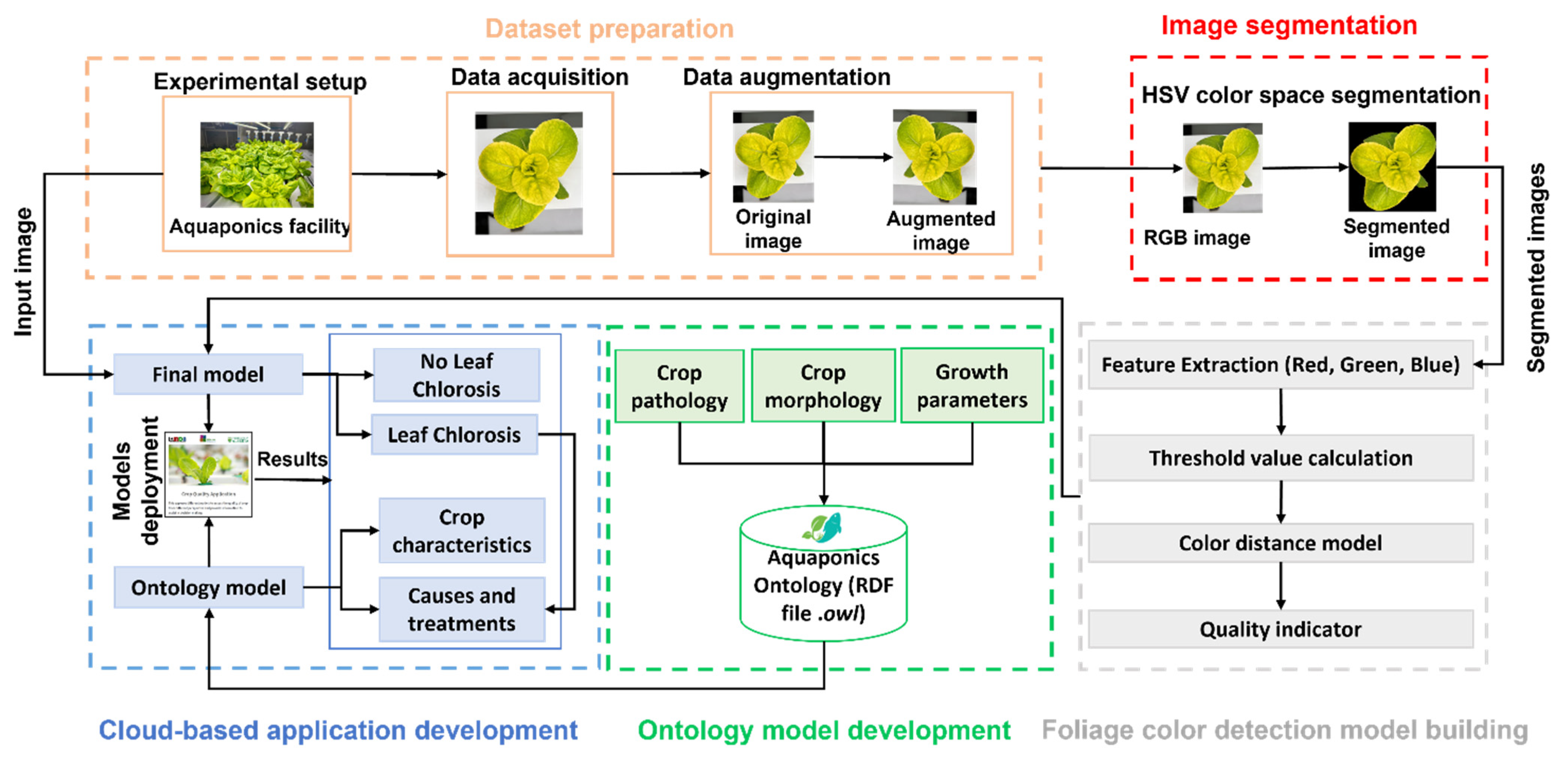
3. Research Methodology

The block diagram, illustrating the five sequential modules of research methodology, is shown in Figure 1. Each module, along with its elements, is described in the next subsections.

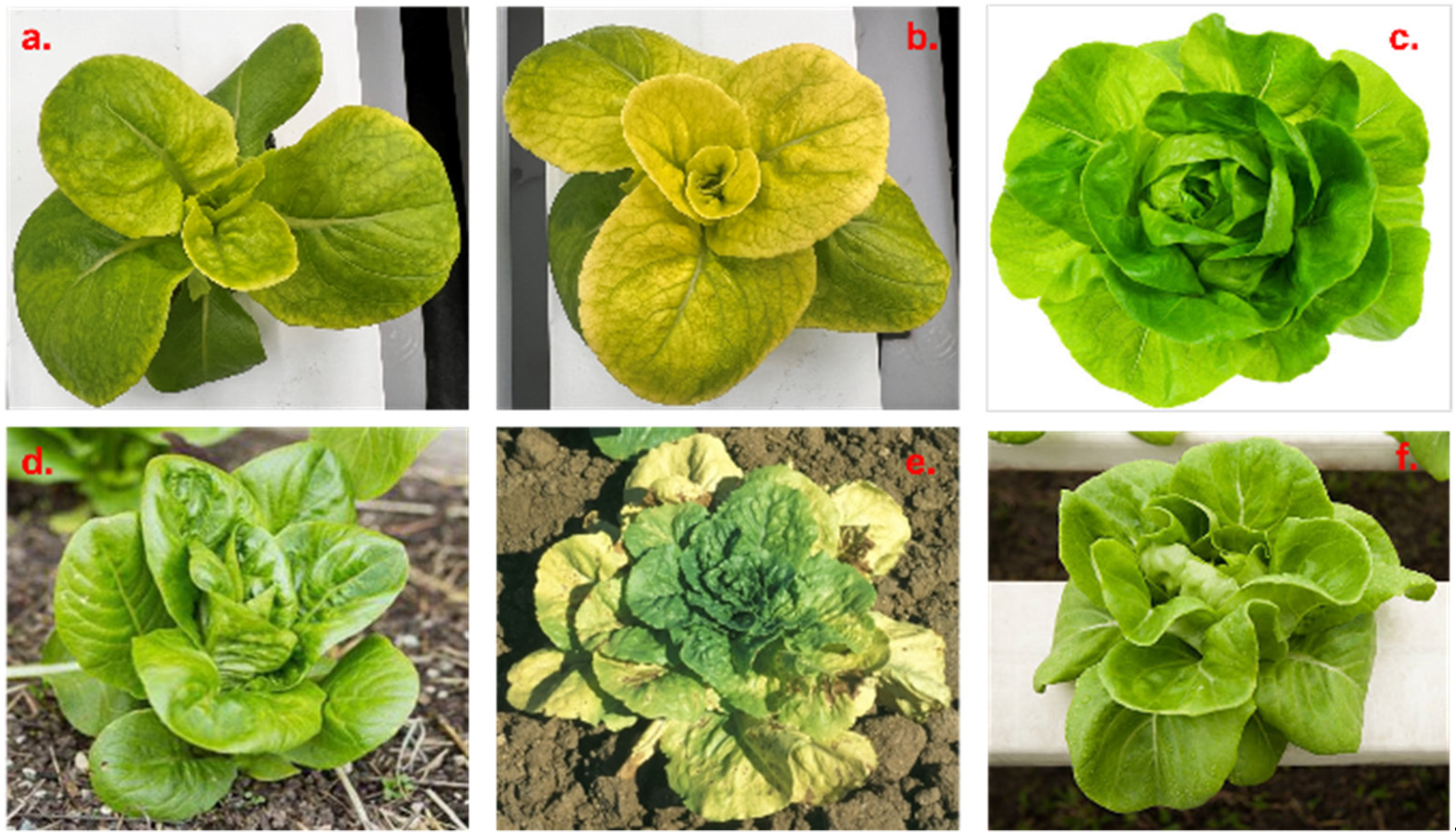
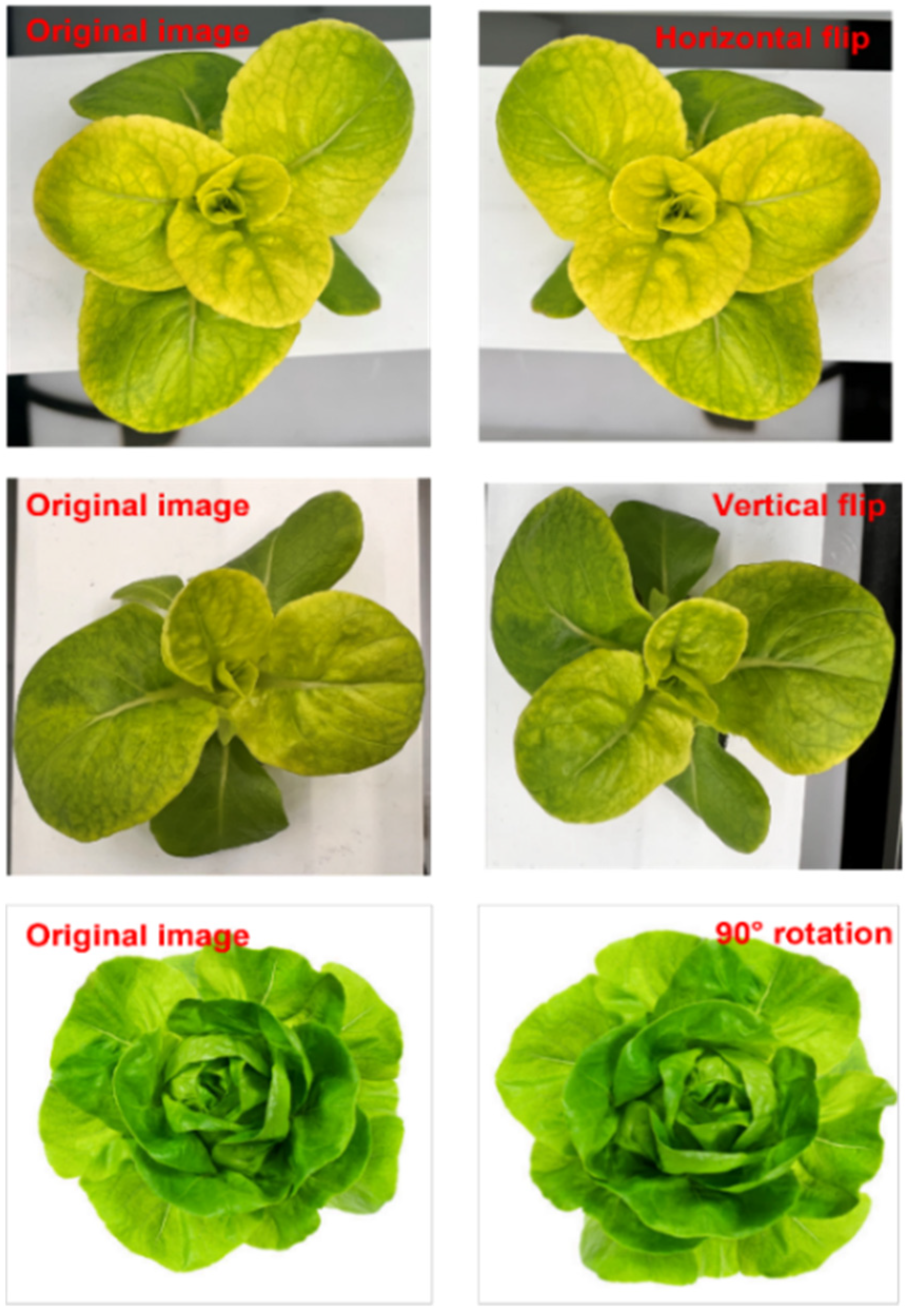
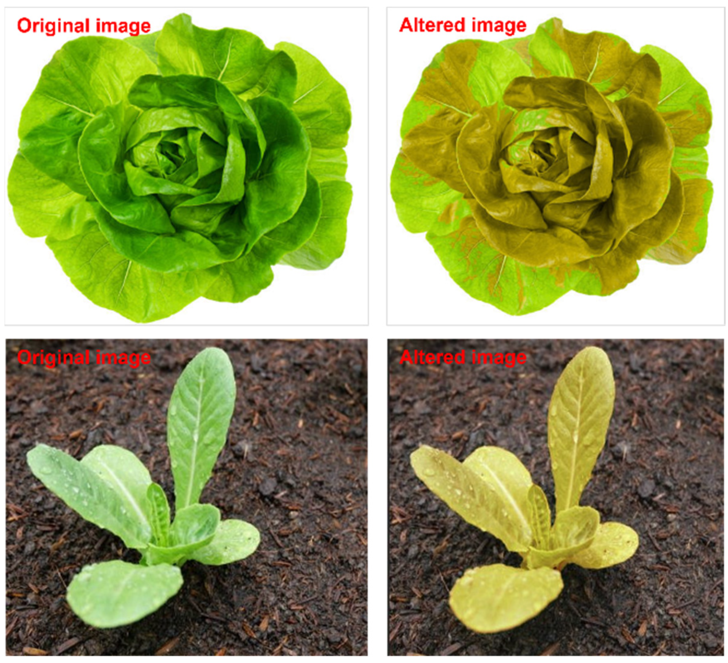
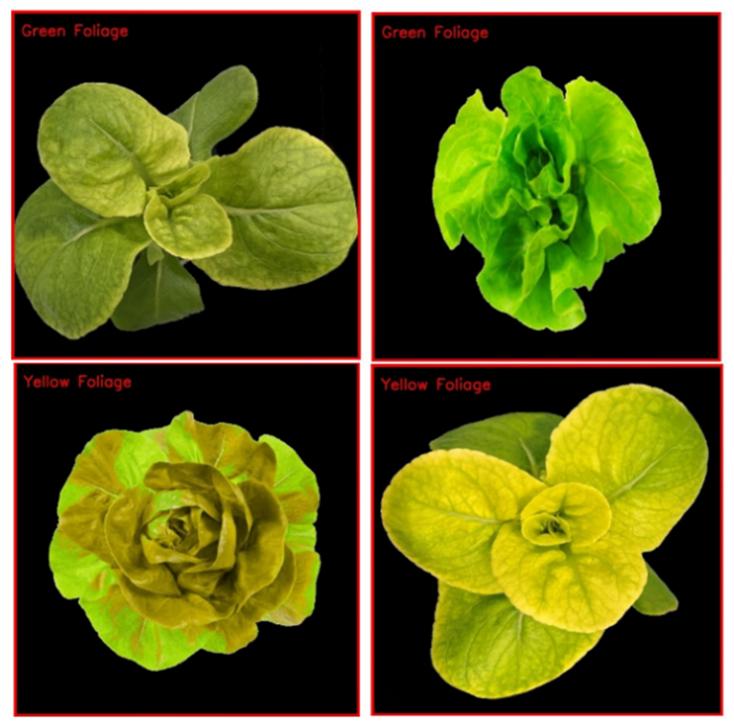
3.1. Data Preparation

The image dataset is constructed using a variety of little gem romaine lettuce images from diverse sources. This involves top-view images of lettuce grown in Allfactory 4.0, an NFT-based aquaponics facility at the University of Alberta, Canada, focusing on smart indoor farming [2]. These images are divided into two classes based on the color of foliage: green foliage (no leaf chlorosis) and yellow foliage (leaf chlorosis). To increase the model flexibility to segment lettuce foliage, irrespective of background, and to ensure it correctly determines the plant’s health, the dataset is complemented with more lettuce images obtained from Ecosia, a search engine based in Berlin, Germany [22]. Figure 2 shows examples of some of the images.

Next, the image augmentation process is performed to increase the dataset and reliability of the segmentation process, despite the location and orientation of the objects in the image, by generating new images from existing images. This study uses Albumentations, a Python library, for fast and flexible image augmentations [23]. The different augmentation techniques applied are the horizontal flip, vertical flip, 90° rotation, and glass noise. The new images are added to their respective classes. Figure 3 shows examples of the augmentations.

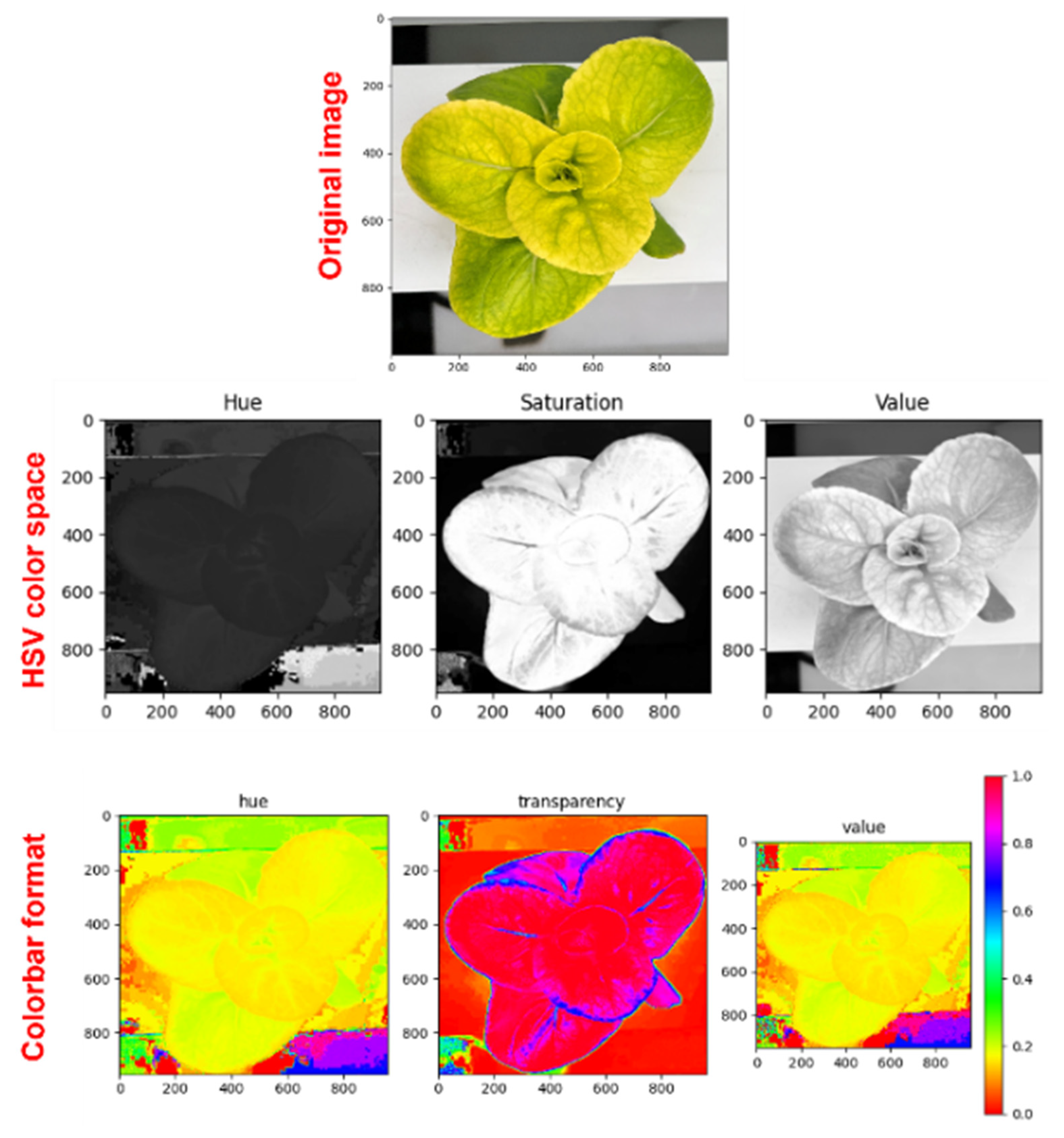
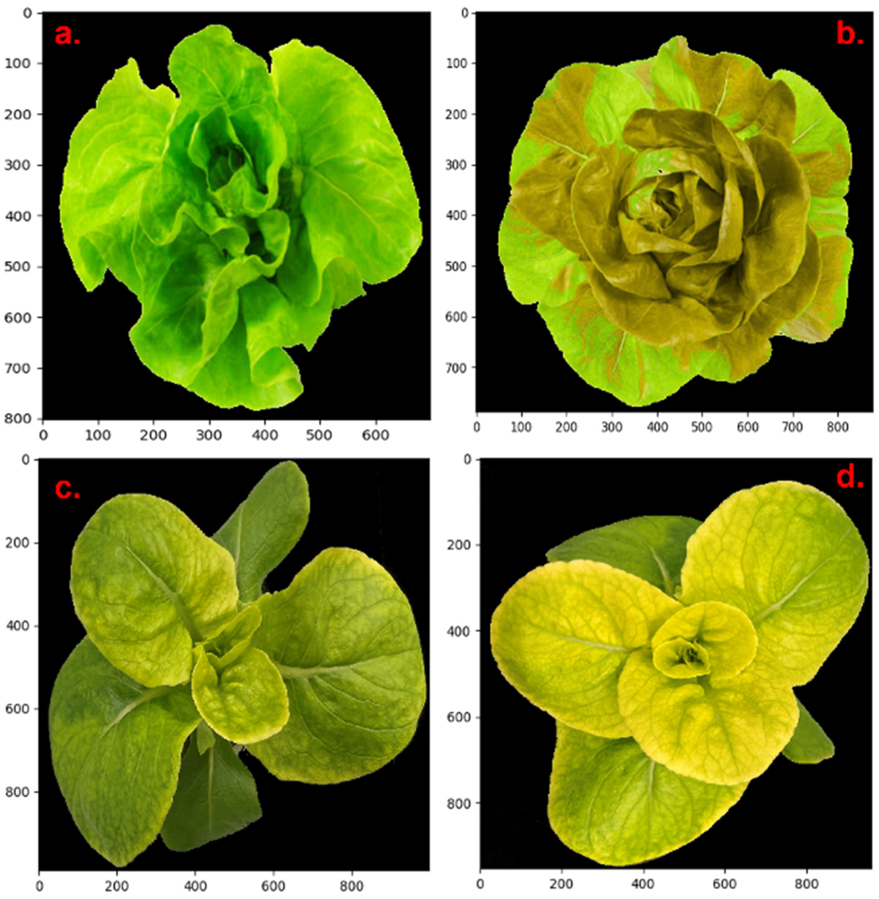
3.2. Image Segmentation

Image segmentation was performed to extract the lettuce foliage from the background for further processing. This study uses the HSV segmentation model to segment the image [16]. There are two stages to the image segmentation process, which are detailed in the next two subsections.

3.2.1. HSV Color Space

The acquired images are in RGB format, where the color of any object in these images is represented with the combined values of the R, G, and B channels. The main problem with this color representation is that the objects’ colors are affected by variations in the illumination conditions [2]. With the HSV color segmentation technique, as the name suggests, HSV color space is used, which describes the objects’ colors independent of the illumination effect [16]. The difference between various color spaces is usually based on color representation. For instance, the object’s color in the HSV color space is represented by three different parameters, namely the hue ($H$), saturation ($S$), and value ($V$). H represents the color of the object, whereas the S and V values represent the illuminance state of the object’s color [16]. This type of description provides the ability to discriminate the color from the illuminance while avoiding the effect of the illumination changes on the object’s color. Therefore, the first stage of segmentation is to convert the image’s color space from RGB into HSV. Generally, the transformation process from RGB into HSV can be performed using the following Equations [24]:

$$R^{\prime }=\frac{R}{255} , G^{\prime }=\frac{G}{255} , B^{\prime }=\frac{B}{255}$$

(1)

$$M=\max \left(R^{\prime }, G^{\prime }, B^{\prime }\right), m=\min \left(R^{\prime }, G^{\prime }, B^{\prime }\right),$$

(2)

$$C=M-m$$

(3)

$$H=\{\begin{array}{c}0° if C=0 \\ 60°\times \left(\frac{G^{\prime }-B^{\prime }}{C}mod 6\right) if M=R^{\prime }\\ 60°\times \left(\frac{G^{\prime }-B^{\prime }}{C}+2\right) if M=G^{\prime }\\ 60°\times \left(\frac{G^{\prime }-B^{\prime }}{C}+4\right) if M=B^{\prime }\end{array}$$

(4)

$$S=\{\begin{array}{c}0 if M=0\\ \frac{C}{M} if M\ne 0\end{array}$$

(5)

$$V=M$$

(6)

After the image transformation, a color bar is created, which provides intensity values for the ($H$), ($S$), and ($V$) channels. These values are used in the next stage for segmenting the image. Figure 4 shows an example of the original image, its HSV channels, and the color bar format.

3.2.2. Image Hue Thresholding

The second stage of image segmentation is to determine the suitable threshold value to distinguish between the foreground and background. For this purpose, the hue image obtained in the first stage is used, as it provides a suitable grayscale image that can be used to classify objects based on color content. The upper and lower range of the hue channels is obtained from the color bar. This range is used to define an upper and lower threshold value for lettuce foliage in a hue image in the form of a mask. This mask is then applied to the R, G, and B channels of the original image, which are then stacked to obtain the segmented image. The final segmented image is saved in RGB format. In order to save time, the segmentation process is automated, and by the end of the process, each segmented image is saved in a common directory.

3.3. Foliage Color Detection Model Development

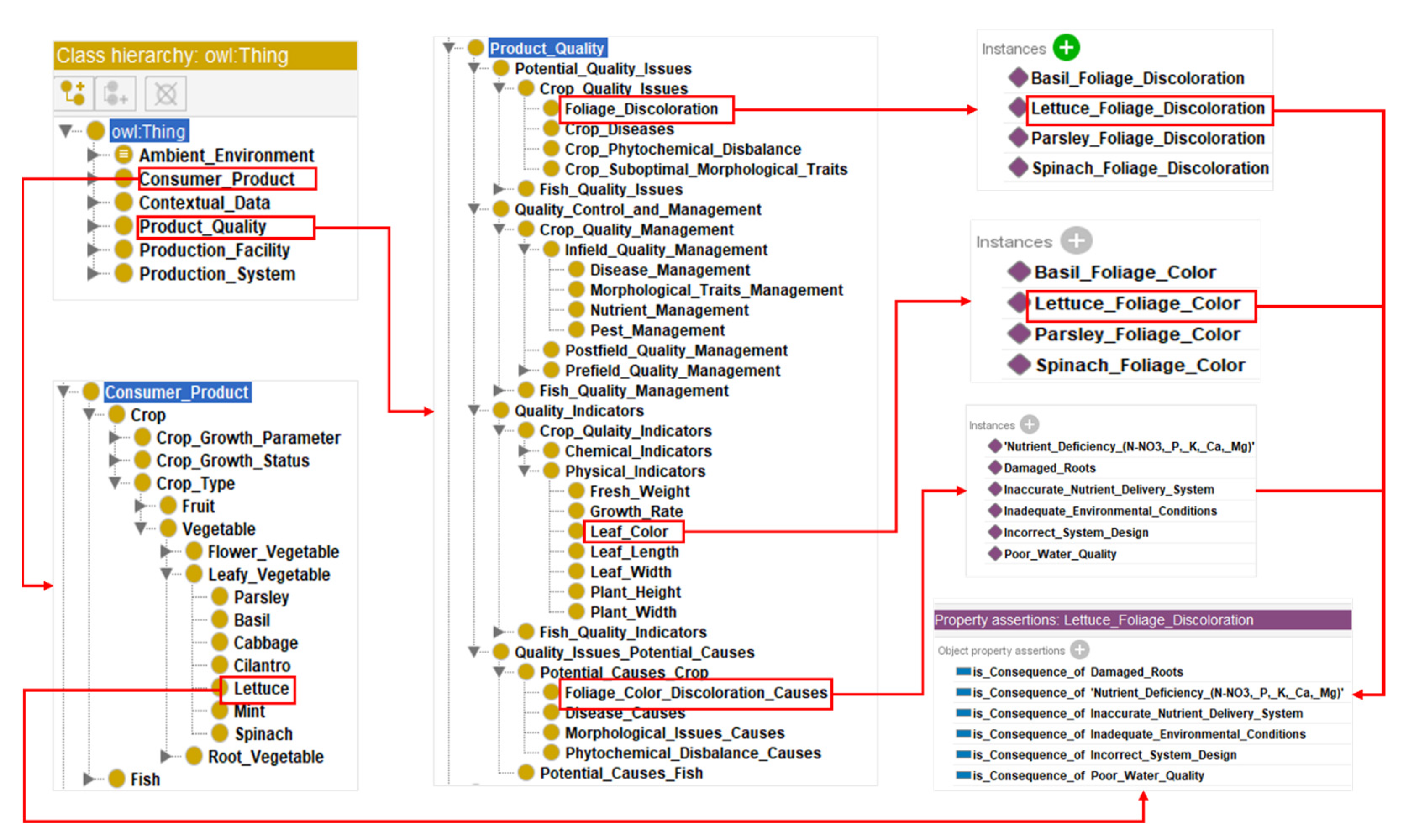
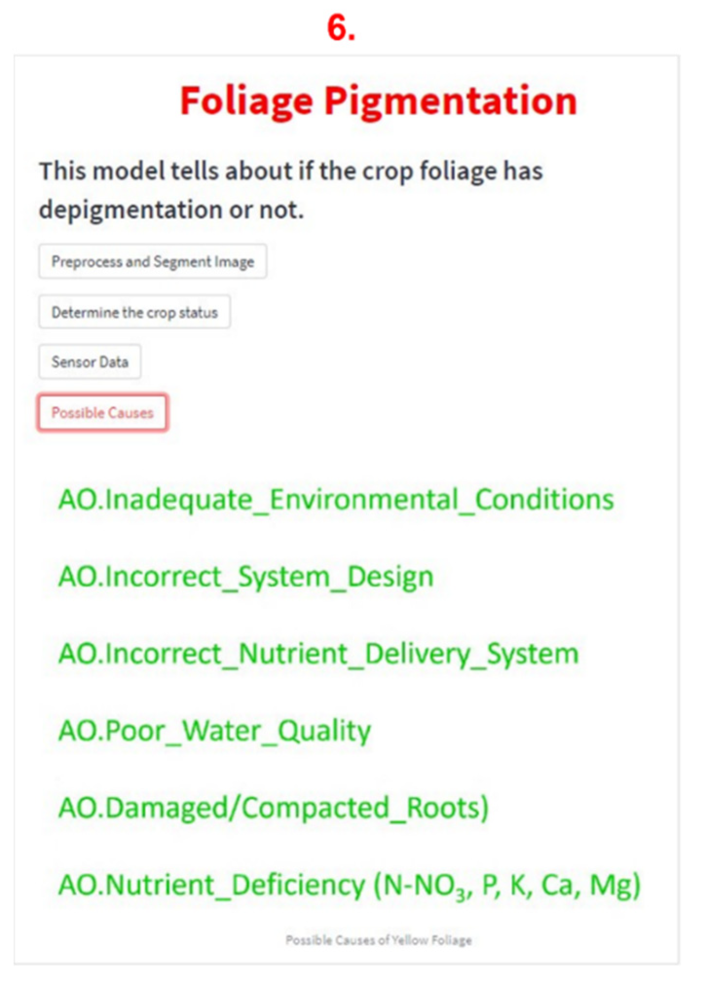
The R, G, and B values of the lettuce foliage (foreground) are extracted from the segmented images. These images are represented as ($i$) and ($j$) for two classes: ($g$) (green foliage—no chlorosis) and ($y$) (yellow foliage—leaf chlorosis), respectively. The mean value of each color channel: red (${\mu }_R$), green (${\mu }_G$), and blue (${\mu }_B$) for the two classes is computed using Equations (1) and (2). The elements of Equations (7) and (8) are determined using Equation (9) through to Equation (14).

$${\mu }_{g,i}=\left[{\mu }_{R,i},{\mu }_{G, i},{\mu }_{B,i}\right]$$

(7)

$${\mu }_{y, j}=\left[{\mu }_{R,j},{\mu }_{G,j},{\mu }_{B,j}\right]$$

(8)

where (${\mu }_{g,i}$) and (${\mu }_{y,j}$) represent the mean values of the three-color channels of the foreground (lettuce foliage) of two classes. Equations (9)–(14) are used for computing the mean values of the channels.

$$R_{i/j}={\sum }_1^{n_{R,i/j}}{R}_{n,i/j}$$

(9)

$$G_{i/j}={\sum }_1^{n_{G,i/j}}{G}_{n,i/j}$$

(10)

$$B_{i/j}={\sum }_1^{n_{B,i/j}}{B}_{n,i/j}$$

(11)

$${\mu }_{R,i/j}=\frac{R_{i/j}}{n_{R,i/j}}$$

(12)

$${\mu }_{G,i/j}=\frac{G_{i/j}}{n_{G,i/j}}$$

(13)

$${\mu }_{B,i/j}=\frac{B_{i/j}}{n_{B,i/j}}$$

(14)

where ($R_{i/j}$), ($G_{i/j}$), and ($B_{i/j}$) refer to the sum of the red, green, and blue values of lettuce foliage in two classes; ($i/j$) refers to either image belonging to the ($g$) class or ($y$) class; and ($n_{R,i/j}$), ($n_{G,i/j}$), and ($n_{B,i/j}$) represent the R, G, and B counts of lettuce foliage, respectively.

The obtained background in segmented images is black. Hence, the R, G, and B counts and values of the background are not included while determining the mean value of the R, G, and B channels for the foreground. The process of calculating the mean values of the R, G, and B channels was, again, automated to save time. The values for each channel were automatically saved in an Excel file. While saving the results, it is ensured that the mean values of R, G, and B are saved for their respective image label and class category, ($g$) and ($y$).

Next, the reference or threshold values (($g_{ref}$) and ($y_{ref}$)) were determined for both ($g$) and ($y$) classes, using Equations (15) and (16). To compute ($g_{ref}$), three average values are calculated, which are related to the mean red, mean green, and mean blue values of the images saved in the Excel file for the ($g$) category. The total number of mean values for each channel is ($m$). The first average value is obtained by summing all the green channel values and dividing the results by the total number of green values ($m$). Similarly, the second and third average values are obtained by summing all the red channel values and all blue channel values of all images in the ($m$) category and dividing the results by the number of red ($m$) and blue values ($m$), respectively. A similar computation is done for ($y_{ref}$) while considering the channel values and their count ($l$) for images in the ($y$) category. Equations (17)–(22) are used to calculate ($g_{ref}$) and ($y_{ref}$).

$$g_{ref}=\left[{\overline{x}}_{R,m},{\overline{x}}_{G, m},{\overline{x}}_{B,m}\right]$$

(15)

$$y_{ref}=\left[{\overline{x}}_{R,l},{\overline{x}}_{G, l},{\overline{x}}_{B,l}\right]$$

(16)

$${\overline{x}}_{R,m}=\frac{{\sum }_1^m{R}_m}{m}$$

(17)

$${\overline{x}}_{G,m}=\frac{{\sum }_1^m{G}_m}{m}$$

(18)

$${\overline{x}}_{B,m}=\frac{{\sum }_1^m{B}_m}{m}$$

(19)

$${\overline{x}}_{R,l}=\frac{{\sum }_1^l{R}_l}{l}$$

(20)

$${\overline{x}}_{G,l}=\frac{{\sum }_1^l{G}_l}{l}$$

(21)

$${\overline{x}}_{B,l}=\frac{{\sum }_1^{l=}{B}_l}{l}$$

(22)

where $({\overline{x}}_{R,m})$, $({\overline{x}}_{G,m})$, and (${\overline{x}}_{B,m})$ are the averages of three channel values in the ($g$) category and $\left(R_m\right)$, $\left(G_m\right)$, and $\left(B_m\right)$, are the values of three channels in the ‘g’ category. Likewise,$({\overline{x}}_{R,l})$, $({\overline{x}}_{G,l})$, and (${\overline{x}}_{B,l})$ are the averages of three channel values in the ($y$) category and $\left(R_l\right)$, $\left(G_l\right)$, and $\left(B_l\right)$, are the values of three channels in the ($y$) category.

After determining the reference or threshold values, the color distance model was used to compute the foliage color difference from the threshold values. The Euclidean distance (ED) model was used in this study, and its general equation is presented below [4].

$$d=\sqrt{\Delta R^2+\Delta G^2+\Delta B^2}$$

(23)

where $\Delta R=R_2-R_1$, $\Delta G=G_2-G_1$, and $\Delta B=B_2-B_1$. Based on the ED model, two distances $\left(d_1\right)$ and $\left(d_2\right)$, were computed using two threshold values: ($g_{ref}$) and ($y_{ref}$), respectively. $\left(d_1\right)$ determines the distance from the green color threshold, whereas $\left(d_2\right)$ determines the distance from the yellow color threshold. For single foliage, both $\left(d_1\right)$ and $\left(d_2\right)$ are determined. A lower value of $\left(d_1\right)$ and a higher value of $\left(d_2\right)$ suggests that the color patterns of foliage are closer to ($g_{ref}$) or, in other words, green tones. Conversely, a lower value of $\left(d_2\right)$ and a higher value of $\left(d_1\right)$ suggests that color patterns of foliage are closer to ($y_{ref}$) or, in other words, yellow tones. The governing equations for $\left(d_1\right)$ and $\left(d_2\right)$ are given below.

$$d_1=\sqrt{{(x_R-{\overline{x}}_{R,m})}^2+{(x_G-{\overline{x}}_{G,m})}^2+{(x_B-{\overline{x}}_{B,m})}^2}$$

(24)

$$d_2=\sqrt{{(x_R-{\overline{x}}_{R,l})}^2+{(x_G-{\overline{x}}_{G,l})}^2+{(x_B-{\overline{x}}_{B,l})}^2}$$

(25)

where $\left(x_R\right)$, $\left(x_G\right)$, and $\left(x_B\right)$ are the mean values of three channels (R, G, B) of the foreground in the segmented image of the test samples.

Lastly, the quality indicator $\left(Q\right)$ is defined as a function of $\left(d_1\right)$ and $\left(d_2\right)$ for evaluating the plants’ quality based on their foliage color. In this context, when green foliage with no leaf depigmentation is detected, the value of $\left(Q\right)$ is equal to 1, which implies that the crop is healthy. On the other hand, when yellow foliage with leaf depigmentation is detected, the value of $\left(Q\right)$ is equal to 0, suggesting that the crop is unhealthy. $\left(Q\right)$ is represented as below:

$$Q=f\left(d_1,d_2\right)=\{\begin{array}{c}1 if d_1<d_2\\ 0 if d_2<d_1\end{array}$$

(26)

3.4. Ontology Model

The complete development and details of all concepts and instances of an ontology model, ‘AquaONT’, is available in previous work by the authors [17]. AquaONT is a unified ontology model that represents and stores the essential knowledge of an aquaponic 4.0 system. It comprises six concepts: Consumer_Product, Ambient_Environment, Contextual_Data, Production_System, Product_Quality, and Production_Facility. In this study, two classes, ‘Consumer_Product’ and ‘Product_Quality’, are used for knowledge extraction. The ‘Consumer_Product’ class provides an abstract view of the type, growth status, and growth parameters of ready-to-harvest crops in an aquaponics system. Whereas the ‘Product_Quality’ class provides knowledge on the crop attributes related to pathology (abiotic and biotic stresses, causes, and the ways and means by which these can be managed or controlled), morphology (canopy dimensions, such as area, length, width, etc.) and foliage color. The lettuce crop is considered in this study. The crop growth and quality attributes are defined as instances of respective classes, which are extracted once the crop foliage is detected as yellow (or leaf chlorosis is detected). Figure 5 shows the hierarchical architecture of the ‘Consumer_Product’ and ‘Product_Quality’ classes, with their instances for the lettuce crop in Protégé7 (an open-source ontology editor and framework developed at Stanford University) environment.

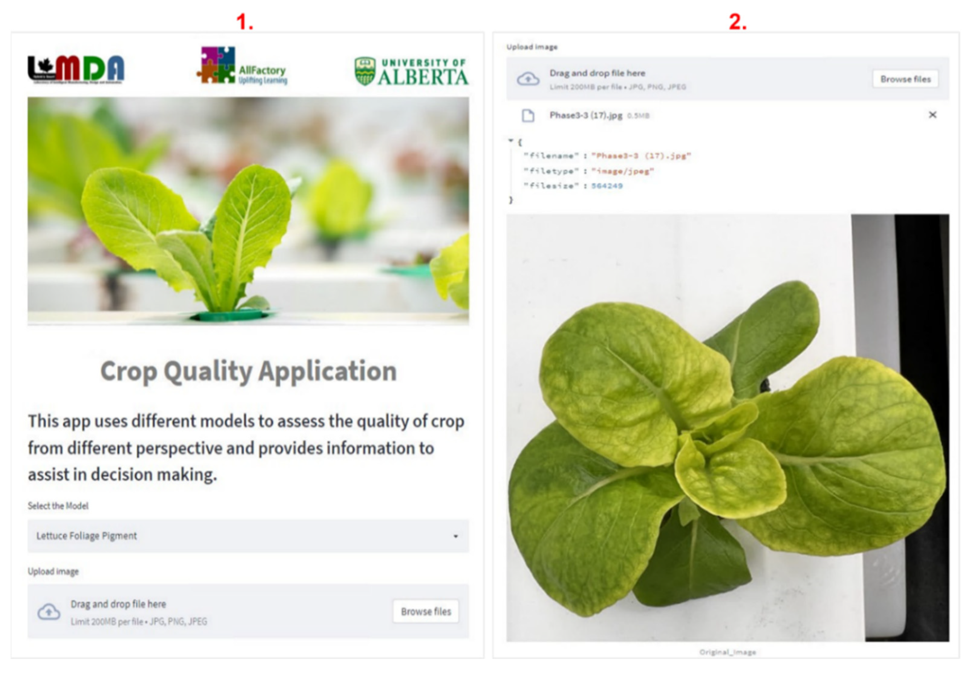
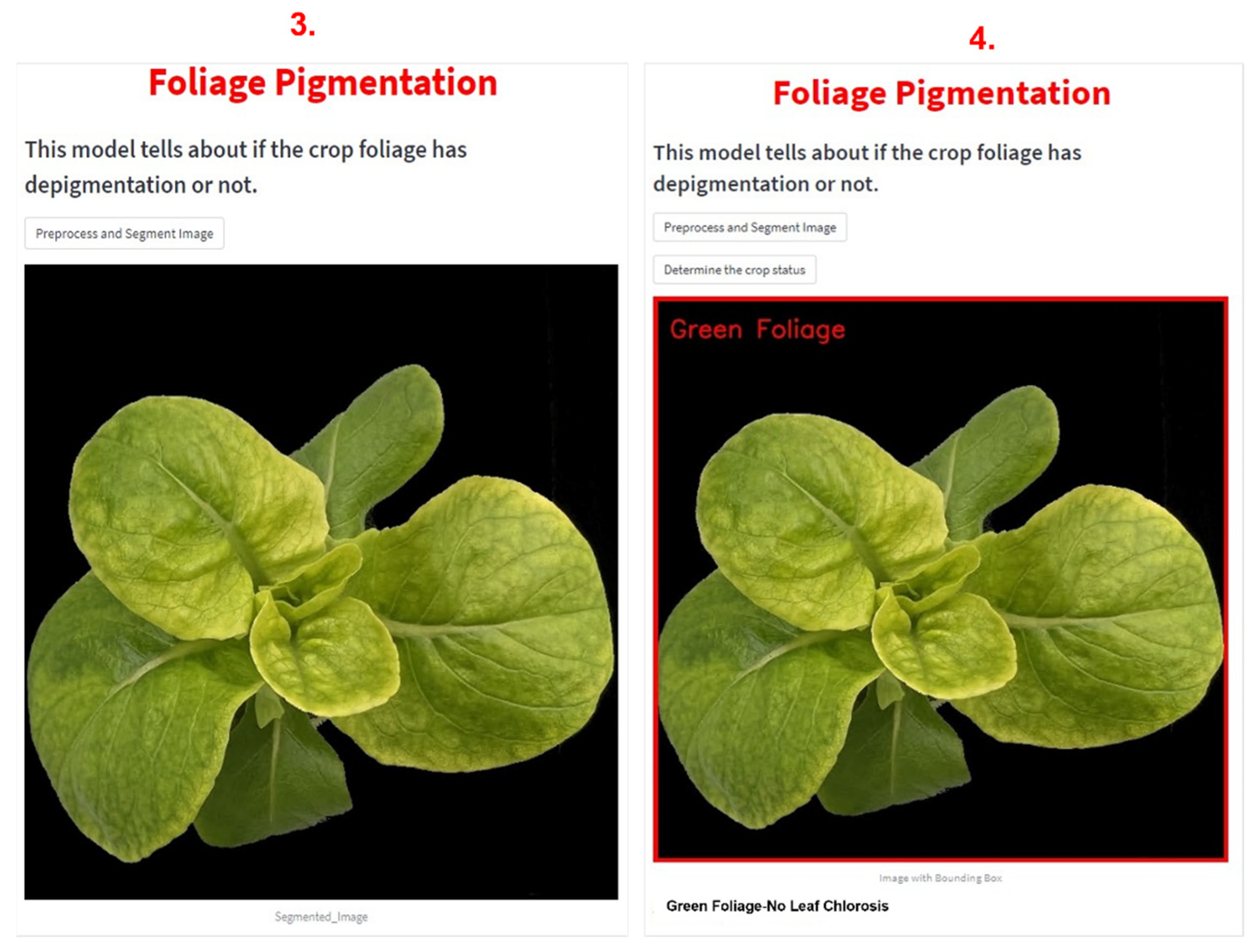
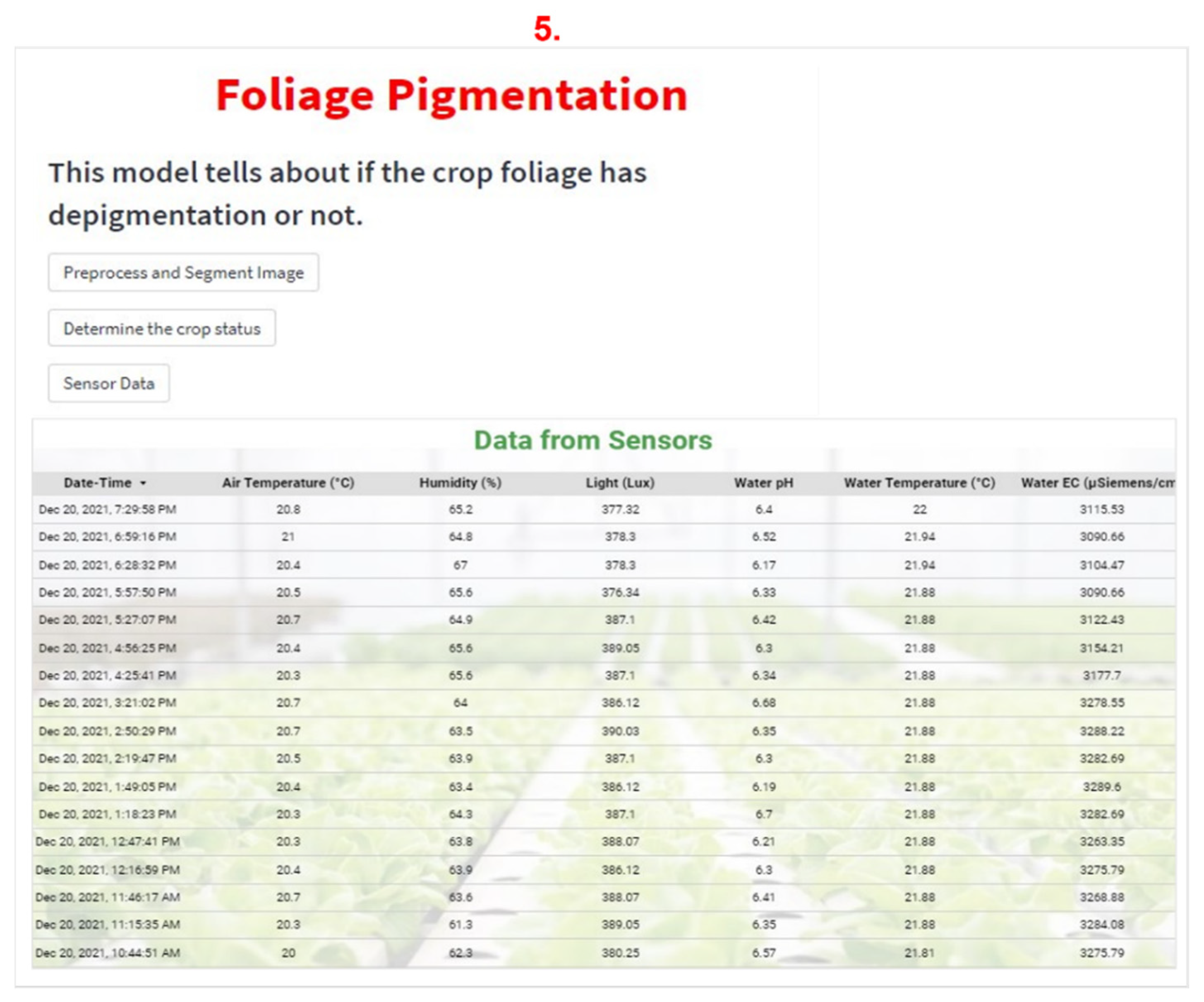
3.5. Cloud-Based Application

The proposed foliage detection and ontology models are deployed on a cloud-based application built on Streamlit. The app’s layout is shown in Figure A1, Figure A2, Figure A3 and Figure A4 in Appendix A. The app works in six stages. The first and second stages are associated with two user inputs, “Select the Model” and “Upload Image”, as shown in Figure A1 in Appendix A. The first input allows the user to select a relevant quality evaluation model. This app has other quality models integrated into it, which are out of the scope of this study. In this study, the relevant model is “Lettuce Foliage Pigment”. After selecting the model, the image is selected using the second input. The third and fourth stages are linked with two widgets, “Preprocess and Segment Image” and “Determine the Crop Status”, respectively, shown in Figure A2 in Appendix A, that run the sub-processes associated with the model. As the name suggests, the first widget activates the segmentation algorithm, which preprocesses and segments the image selected by the user in the second stage. Likewise, the second widget activates the model developed in the study. The model determines the status of the crop and displays the results on the application panel. In the fifth stage, the sensor data from the dashboard is acquired and displayed to monitor the environmental conditions, as shown in Figure A3 in Appendix A. By clicking ‘Sensor Data’, the most recent data will be displayed. In the sixth stage, a widget is developed, ‘Causes and Treatments’, which is linked with ‘AquaONT’. This widget extracts knowledge from the ontology model related to the possible causes of leaf yellowing in the aquaponics facility. Figure A4 in Appendix A show the sixth stage of the app when yellow foliage is detected.

4. Results and Discussion

This section first presents the validation of the proposed method by a case study. Then, the performance of the proposed method is compared with existing similar methods.

To validate the proposed model, twenty healthy seedings were placed in NFT-based hydroponic systems for five weeks (plantation cycle), after which lettuce was harvested. A 12MP Sony Exmor RS camera sensor was used to capture the crop images during this period. Twenty images of 4032 × 3024 pixels (one image for one lettuce plant) were captured daily at 9:00 am from the top while keeping the distance between the camera and channel at a value of 40 cm throughout the plantation cycle, i.e., five weeks. In total, 700 images of plants were collected over five weeks. During the first three weeks, no significant difference was observed in the color of the foliage. After the third week, foliage chlorosis was observed in eight lettuce plants. Therefore, for further processing, the images captured in the last two weeks of the plantation cycle were considered for model validation. In total, 280 images were divided into two classes based on the color of the foliage: Green Foliage—No Leaf Chlorosis (168 images) and Yellow Foliage—Leaf Chlorosis (112 images). The dataset is complemented with more lettuce images with green (32) and yellow (88) foliage, downloaded from Ecosia. The images were added to their respective classes. All the images were resized to 1000 × 1000 pixels and saved in JPG format. The augmentation process was then performed. In total, 100 images (50 from both classes) were selected randomly for the augmentation, which created 100 new images. The new images were added to their respective classes, increasing the length of the dataset to 500 images. Half of these images belong to the ($g$) class, and half belong to the ($y)$ class and, hence, are saved in two folders named ($g$) and ($y),$ respectively. Out of 500 images, 100 random images (50 from each folder) were extracted and saved in a separate validation folder to be used for the model evaluation. In order to complement the validation data, 20 images were randomly selected (10 from each class), and their R, G, and B values were altered using Adobe Photoshop in a way that the healthy-looking lettuce appears yellow, and the unhealthy lettuce appears green. The validation dataset now had 120 images in total. Figure 6 shows an example of the new images generated for the validation dataset.

The segmentation was then performed on all 520 images in the dataset. Figure 7 shows an example of the segmented images. For the computation of the threshold values, 400 images (g and y folder) were used by following the process mentioned in Section 3.3. The R, G, and B values and their counts were computed for the foreground (lettuce foliage) of 400 segmented images in two classes, ($g$) and ($y$). The mean values of the R, G, and B channels were then computed. Each class has 200 foliage images, so for each class 3 × 200 = 600 mean values (3 refers to 3 channels of an image) were obtained, which were automatically saved in an excel file.

Out of the 600 means values for each class, 200 belong to the red channel, 200 belong to the green channel, and 200 belong to the blue channel. The threshold values ($g_{ref}$) and ($y_{ref}$) were obtained by dividing the mean values of the three channels by 200, which are given below.

$$g_{ref}=\left[{\overline{x}}_{R,m},{\overline{x}}_{G, m},{\overline{x}}_{B,m}\right]=\left[123.4, 138.2, 19.8\right]$$

(27)

$$y_{ref}=\left[{\overline{x}}_{R,l},{\overline{x}}_{G, l},{\overline{x}}_{B,l}\right]=\left[156.6, 155.8, 22.2\right]$$

(28)

The model was validated using a validation dataset comprising 120 different segmented images belonging to two classes, ($g$) and ($y)$. The mean values of the three channels were computed for each image and were inserted into Equations (27) and (28) in place of $\left(x_R\right)$, $\left(x_G\right)$, and $\left(x_B\right)$, along with the reference values ($g$) and ($y)$ computed above. The $\left(d_1\right)$ and $\left(d_2\right)$ were determined for all 120 images in the validation dataset using Equations (17) and (18), respectively. The quality indicator, $\left(Q\right)$, was also determined using Equation (19) for 120 images. The performance of the model on the validation dataset was then evaluated by analyzing the ground truth $\left(Q\right)$ value and predicted $\left(Q\right)$ value. In the validation dataset, 60 images have a ground truth $\left(Q\right)$ value of 1, meaning these images contain healthy and green lettuce foliage, and 60 images have a ground truth value of 0, meaning these Images contain unhealthy and yellow lettuce foliage. The performance is presented in the form of a confusion matrix (CM), shown in Figure 8 [2].

The different values of the CM are interpreted as:

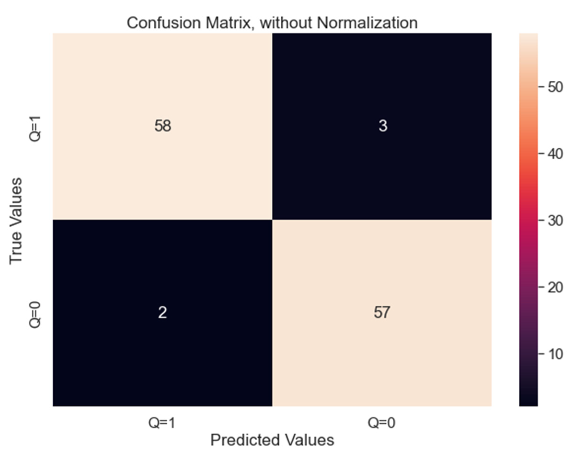
• True Positive (TP) = 58. Thus, 58 plants were healthy, and the model correctly classified them healthy as well.
• True Negative (TN) = 57. Thus, 57 plants were unhealthy, and the model correctly classified them unhealthy as well.
• False Positive (FP) = 3. Thus, 3 plants were unhealthy, but the model incorrectly classified them as healthy.
• False Negative (FN) = 2. Thus, 2 plants were healthy, but the model incorrectly classified them as unhealthy.

The performance metrics based on CM are also computed using the formulae given below and are summarized in

Table 1. Summary of the performance metrics.

Class	N (Truth)	N (Classified)	Accuracy	Precision	Recall	F1-Score
Q = 1	60	61	0.95	0.95	0.97	0.96
Q = 0	60	59	0.95	0.97	0.95	0.96
Average	-	-	0.95	0.96	0.96	0.96

.

$$Accuracy=\frac{TP+TN}{TP+TN+FP+FN}$$

(29)

$$Precision=\frac{TP}{TP+FP}$$

(30)

$$Recall=\frac{TP}{TP+FN}$$

(31)

$$F1-Score=\frac{2\times Precision\times Recall}{Precision+Recall}$$

(32)

In Table 1, N (truth) tells the number of actual cases in a particular class, and N (classified) tells the number of predicted cases belonging to a class. Table 1 shows that the model has achieved an average accuracy of 95%, precision of 96%, recall of 96%, and F1-Score of 96%. The model has correctly classified 115 cases out of a total of 120 cases. Figure 9 shows an example of correctly classified cases.

To further investigate the performance of the proposed methodology, it was compared with the existing vision-based methods mentioned in Section 2. These methods were implemented on the dataset prepared in this study, and their performance was evaluated using the metrics based on CM, which are presented in

Table 2. Performance metrics of existing methods.

Methods	Techniques and Parameters Used	Average Accuracy	Average Precision	Average Recall	Average F1-Score
Yang et al. [18]	SVM (support vector machine) and a* (CIELAB color space), G (green from RGB color space), and H (hue from HSV color space)	0.91	0.92	0.93	0.925
Maity et al. [19]	Otsu’s method and k-means clustering technique	0.92	0.93	0.93	0.93
Yang et al. [20]	HSV (hue, saturation, and value) color space and decision tree method	0.89	0.91	0.90	0.905
Luna-Benoso et al. [21]	Otsu’s method, SVM, k-NN (k-nearest neighbor) and MLP (multi-layer perceptron)	0.90	0.91	0.91	0.91
Hasan et al. [25]	L*a*b* color histogram, k-NN, and random forest	0.94	0.95	0.94	0.945
-	Proposed model	0.95	0.96	0.96	0.96

. The results show that the proposed method has outperformed the similar existing methods, achieving an average accuracy of 96%, precision, recall, and F1-score of 96%. The method proposed by Sharad et al. has shown appreciable performance when implemented on the dataset prepared in this study by achieving an average accuracy of 94%, a precision of 94%, a recall of 95%, and an F1-score of 94.45% [25]. Whereas, with their apple leaf dataset, they have achieved an accuracy of 98.63%.

The final model was then deployed in the aquaponics facility through a cloud-based application. This time, instead of manually taking the images, four ELP 1080P webcams (2.8–12 mm HD Varifocal Lens) were installed at a distance of 40 cm from the channels for image acquisition. Each camera is programmed through a Raspberry Pi 4 (Model B Rev 1) controller to take one image per day at 9:00 am, which along with the sensor values from WSM, are wirelessly uploaded to the ‘IoT enabled Aquaponics Dashboard’ developed by the authors in previous work [26]. The images and sensor data are available on the cloud as well as locally, and the app developed in this study can access them. The ontology model discussed in Section 3.4 was also integrated with the proposed model and deployed on a cloud-based application. Once the health status of the lettuce crop was identified as ‘Yellow Foliage—Leaf Chlorosis’, the potential causes were automatically extracted from the ontology model and displayed on the application panel. Figure A1, Figure A2, Figure A3 and Figure A4 in Appendix A show an example of the working of the proposed method and application for a lettuce crop when its foliage was detected to be yellow. The primary causes of lettuce foliage chlorosis could be inadequate environmental conditions (humidity, air temperature), poor water quality (inadequate pH or EC), nutrient deficiency, etc. By analyzing sensor data and the possible causes of leaf chlorosis, it is possible to reach the specific cause of the problem. For instance, if sensor data show that all the parameters are within their optimal ranges, then the problem could be related to nutrient delivery or the design of the system. A reasonable treatment can be suggested after problem identification.

The proposed model was developed using open-source frameworks, and, hence, it can easily be expanded or adjusted as per the requirement by adjusting the threshold values. The significance of the model is that it is fully automated and offers a non-destructive, low-cost and reliable approach to identifying leaf chlorosis and determining the quality of lettuce plants along with the possible causes. In contrast to the computer vision and machine learning-based models, the proposed methodology requires less data.

5. Conclusions

This study discusses the major problem of lettuce foliage chlorosis in an aquaponics context. The ‘HSV Color Segmentation’ image processing approach was used to segment the lettuce images obtained from various resources. The segmented images were divided into two classes, ‘Green Foliage-No Leaf Chlorosis’ and ‘Yellow Foliage-Leaf Chlorosis’. Then, the foliage color detection model was developed, and a quality indicator was defined to identify leaf chlorosis and determine the quality of the lettuce crop. The model is validated, achieving an overall accuracy of 95%. The performance of the model was also compared with existing similar methods. The results show that the proposed method has outperformed these existing methods. A cloud-based application was then developed, where the final model was deployed. The ontology model that contains knowledge related to the causes of lettuce crop chlorosis was also integrated with the final model. The proposed system proves to be accurate and flexible enough to be used in real scenarios and, hence, is not limited to being disturbed by potentially changing conditions and environments.

For future work, the system will be extended to include other crops. Moreover, images with complex backgrounds and multiple objects will also be added to the dataset. The ontology model will also be extended to include the specific treatments for potential causes of leaf chlorosis.

References

1. Abbasi, R.; Martinez, P.; Ahmad, R. An ontology model to support the automated design of aquaponic grow beds. Procedia CIRP 2021, 100, 55–60. [Google Scholar] [CrossRef]
2. Reyes-Yanes, A.; Martinez, P.; Ahmad, R. Real-time growth rate and fresh weight estimation for little gem romaine lettuce in aquaponic grow beds. Comput. Electron. Agric. 2020, 179, 105827. [Google Scholar] [CrossRef]
3. Lin, K.H.; Huang, M.Y.; Huang, W.D.; Hsu, M.H.; Yang, Z.W.; Yang, C.M. The effects of red, blue, and white light-emitting diodes on the growth, development, and edible quality of hydroponically grown lettuce (Lactuca sativa L. var. capitata). Sci. Hortic. 2013, 150, 86–91. [Google Scholar] [CrossRef]
4. Haider, T.; Farid, M.S.; Mahmood, R.; Ilyas, A.; Khan, M.H.; Haider, S.T.A.; Chaudhry, M.H.; Gul, M. A Computer-Vision-Based Approach for Nitrogen Content Estimation in Plant Leaves. Agriculture 2021, 11, 766. [Google Scholar] [CrossRef]
5. Taha, M.F.; Abdalla, A.; Elmasry, G.; Gouda, M.; Zhou, L.; Zhao, N.; Liang, N.; Niu, Z.; Hassanein, A.; Al-Rejaie, S.; et al. Using Deep Convolutional Neural Network for Image-Based Diagnosis of Nutrient Deficiencies in Plants Grown in Aquaponics. Chemosensors 2022, 10, 45. [Google Scholar] [CrossRef]
6. Matysiak, B.; Ropelewska, E.; Wrzodak, A.; Kowalski, A.; Kaniszewski, S. Yield and Quality of Romaine Lettuce at Different Daily Light Integral in an Indoor Controlled Environment. Agronomy 2022, 12, 1026. [Google Scholar] [CrossRef]
7. Abbasi, R.; Martinez, P.; Ahmad, R. The digitization of agricultural industry—A systematic literature review on agriculture 4.0. Smart Agric. Technol. 2022, 2, 100042. [Google Scholar] [CrossRef]
8. Kowalczyk, K.; Sieczko, L.; Goltsev, V.; Kalaji, H.M.; Gajc-Wolska, J.; Gajewski, M.; Gontar, Ł.; Orliński, P.; Niedzińska, M.; Cetner, M.D. Relationship between chlorophyll fluorescence parameters and quality of the fresh and stored lettuce (Lactuca sativa L.). Sci. Hortic. 2018, 235, 70–77. [Google Scholar] [CrossRef]
9. Song, J.; Huang, H.; Hao, Y.; Song, S.; Zhang, Y.; Su, W.; Liu, H. Nutritional quality, mineral and antioxidant content in lettuce affected by interaction of light intensity and nutrient solution concentration. Sci. Rep. 2020, 10, 2796. [Google Scholar] [CrossRef] [Green Version]
10. Cook, S.E.; Bramley, R.G.V. Coping with variability in agricultural production -implications for soil testing and fertiliser management. Commun. Soil Sci. Plant Anal. 2000, 31, 1531–1551. [Google Scholar] [CrossRef]
11. Kjeldahl, J. Neue Methode zur Bestimmung des Stickstoffs in organischen Körpern. Z. Anal. Chem. 1883, 22, 366–382. [Google Scholar] [CrossRef] [Green Version]
12. Yang, W.H.; Peng, S.; Huang, J.; Sanico, A.L.; Buresh, R.J.; Witt, C. Using Leaf Color Charts to Estimate Leaf Nitrogen Status of Rice. Agron. J. 2003, 95, 212–217. [Google Scholar] [CrossRef]
13. Markwell, J.; Osterman, J.C.; Mitchell, J.L. Calibration of the Minolta SPAD-502 leaf chlorophyll meter. Photosynth. Res. 1995, 46, 467–472. [Google Scholar] [CrossRef]
14. Zheng, H.; Cheng, T.; Li, D.; Zhou, X.; Yao, X.; Tian, Y.; Cao, W.; Zhu, Y. Evaluation of RGB, Color-Infrared and Multispectral Images Acquired from Unmanned Aerial Systems for the Estimation of Nitrogen Accumulation in Rice. Remote Sens. 2018, 10, 824. [Google Scholar] [CrossRef] [Green Version]
15. Tao, M.; Ma, X.; Huang, X.; Liu, C.; Deng, R.; Liang, K.; Qi, L. Smartphone-based detection of leaf color levels in rice plants. Comput. Electron. Agric. 2020, 173, 105431. [Google Scholar] [CrossRef]
16. Burdescu, D.D.; Brezovan, M.; Ganea, E.; Stanescu, L. A new method for segmentation of images represented in a HSV color space. In Proceedings of the Advanced Concepts for Intelligent Vision Systems: 11th International Conference, ACIVS 2009, Bordeaux, France, 28 September–2 October 2009; Springer: Berlin/Heidelberg, Germany, 2009; pp. 606–617. [Google Scholar] [CrossRef]
17. Abbasi, R.; Martinez, P.; Ahmad, R. An ontology model to represent aquaponics 4.0 system’s knowledge. Inf. Process. Agric. 2022, 9, 514–532. [Google Scholar] [CrossRef]
18. Yang, R.; Wu, Z.; Fang, W.; Zhang, H.; Wang, W.; Fu, L.; Majeed, Y.; Li, R.; Cui, Y. Detection of abnormal hydroponic lettuce leaves based on image processing and machine learning. Inf. Process. Agric. 2021, 10, 1–10. [Google Scholar] [CrossRef]
19. Maity, S.; Sarkar, S.; Vinaba Tapadar, A.; Dutta, A.; Biswas, S.; Nayek, S.; Saha, P. Fault Area Detection in Leaf Diseases Using K-Means Clustering. In Proceedings of the 2018 2nd International Conference on Trends in Electronics and Informatics (ICOEI), Tirunelveli, India, 11–12 May 2018; pp. 1538–1542. [Google Scholar] [CrossRef] [Green Version]
20. Yang, W.; Wang, S.; Zhao, X.; Zhang, J.; Feng, J. Greenness identification based on HSV decision tree. Inf. Process. Agric. 2015, 2, 149–160. [Google Scholar] [CrossRef] [Green Version]
21. Luna-Benoso, B.; Martínez-Perales, J.C.; Cortés-Galicia, J.; Flores-Carapia, R.; Silva-García, V.M. Detection of Diseases in Tomato Leaves by Color Analysis. Electronics 2021, 10, 1055. [Google Scholar] [CrossRef]
22. Streamlit • The Fastest Way to Build and Share Data Apps [WWW Document], n.d. Available online: https://streamlit.io/ (accessed on 7 June 2022).
23. Buslaev, A.; Iglovikov, V.I.; Khvedchenya, E.; Parinov, A.; Druzhinin, M.; Kalinin, A.A. Albumentations: Fast and flexible image augmentations. Information 2020, 11, 125. [Google Scholar] [CrossRef] [Green Version]
24. Loresco, P.J.M.; Valenzuela, I.C.; Dadios, E.P. Color Space Analysis Using KNN for Lettuce Crop Stages Identification in Smart Farm Setup. In Proceedings of the TENCON 2018-2018 IEEE Region 10 Conference, Jeju, Republic of Korea, 28–31 October 2018; pp. 2040–2044. [Google Scholar] [CrossRef]
25. Hasan, S.; Jahan, S.; Islam, M.I. Disease detection of apple leaf with combination of color segmentation and modified DWT. J. King Saud Univ.-Comput. Inf. Sci. 2022, 34, 7212–7224. [Google Scholar] [CrossRef]
26. Abbasi, R.; Martinez, P.; Ahmad, R. Data acquisition and monitoring dashboard for IoT enabled aquaponics facility. In Proceedings of the 2022 10th International Conference on Control, Mechatronics and Automation (ICCMA), Luxembourg, 9–12 November 2022; IEEE: Piscataway, NJ, USA, 2022. [Google Scholar] [CrossRef]
Figure 1. Research methodology outline.
Agriculture 13 00615 g001
Figure 2. Image dataset: (a,b) acquired from aquaponics facility, and (cf) are downloaded from ecosia.org.
Agriculture 13 00615 g002
Figure 3. Data augmentation was performed on different images.
Agriculture 13 00615 g003
Figure 4. Illustration of image, its HSV channels, and color bar format.
Agriculture 13 00615 g004
Figure 5. Ontology model showing classes, instances, and relationships between them.
Agriculture 13 00615 g005
Figure 6. Example of images generated in Adobe Photoshop (left original images, right for the altered images).
Agriculture 13 00615 g006
Figure 7. Example of segmented images ((a,c): segmented green lettuce; (b,d): segmented altered yellowed lettuce).
Agriculture 13 00615 g007
Figure 8. Confusion Matrix.
Agriculture 13 00615 g008
Figure 9. Example of correctly classified cases.
Agriculture 13 00615 g009