1. Introduction
As the concept of competitiveness is highly controversial, it is often described as “confusing and unclear” [
1]. An examination of recent developments in regional industrial policy in the United Kingdom reveals that competitiveness is synonymous with productivity growth [
2]. As per an integrated concept of competitiveness, a competitiveness strategy is “right and useful” as long as it is effective in providing a practical function for industry [
3].
The OECD suggested that “competitiveness” be understood as: “…the ability of companies, etc., to generate while being and remaining exposed to international competition, relatively high factor income, and factor employment levels on a sustainable basis.” [
4]. The World Economic Forum has defined “competitiveness” as “the set of institutions, policies, and factors that determine the level of productivity of a country, in an effort to understand and measure the drivers of economic prosperity”. Blanke, et al. [
5] expanded sustainable competitiveness (SCI) to make competitiveness sustainable over the longer run, in economic, social, and environmental terms.
Adopting sustainable management has been considered a critical way for companies to operate in the current business environment [
6,
7]. Lacy, et al. [
8] survey of 766 Global Compact member CEOs from nearly 100 countries showed that 96% of CEOs believe that sustainability issues should be fully integrated into the strategy and operations of a company. There is a positive relationship between sustainable innovation and corporate competitiveness, which can create a win–win situation for companies [
9].
The competitive strategy of a firm that is active only in local marketplaces, is affected by its competitive environment naturally [
10]. It requires sufficient resources to effectively enforce competition law [
11]. The challenge of sustainable competitiveness is not only in designing an analytical framework but also in selecting a suitable measurement approach [
12]. In short, The most important issue is to find out the factors which create the complex competitive advantage of the region regarding economic, performance, social goals, or different geographies, etc. [
13].
Many successful and innovative companies now formulate their strategic business models with conventional operations such as “At Zara, the supply chain is the business model” [
7]. Bublyk, et al. [
14] used cluster analysis and the fuzzy C-means (FCM) clustering approach to group economic activities and identified two groups of industries in Ukraine, namely, mining, and quarrying industries and electricity, natural gas, steam, and air conditioning supply industries, as environmentally unfriendly industries, given the high degree of damage they cause to resources during the production process. Based on the findings, timely problem management was proposed as a solution for these industries. Battermann, et al. [
15] analyzed the differences and conflicts among residents concerning the developmental direction during the development process in the rural areas of Lower Saxony, Germany. They confirmed the existence of cluster structures through the analysis of agricultural structures and production differences, and then recombined their findings through a discussion about the clusters to propose viable economic alternatives.
Business models are not a completely new concept [
16], but are included in strategy theory [
17]. Maintaining the profits of those who are connected in the supply chain is the key element to maintain long-term business success [
18]; for this reason, the competitiveness reports published by the World Competitiveness Center at the International Institute for Management Development are widely used in different fields as a key to examining the enhancement of the competitiveness of countries or companies. Cluster analysis can also be used to understand the differences between technological innovation and competitiveness to develop strategic policies [
19].
Rural policies in many countries have undergone major shifts over the past two decades. Agricultural policy objectives focus more on improving the competitiveness of agricultural businesses in rural areas, diversifying economic activities and finding niche markets for local products [
20]. Therefore, policy is required to be effective and transferable to prompt the local farming organization to face environmental changes by improving performance [
21]. If supply chain performance is an expression of national competitiveness, the businesses that finance and manage supply chains are important, especially in agriculture when it comes to food supply and quality [
22].
Taiwan Farmers’ Associations (TFAs) constitute the most important nonprofit organizations influencing agricultural development in Taiwan, with a history of 120 years since the first farmers’ association was established in 1900. A TFA is divided into three levels according to the administrative hierarchy, each operating independently. In 2022, there were 302 associations, including 279 local TFAs (LTFAs) at the township/city/district level, with a total membership of approximately 1.7 million. However, because of the lack of a fair assessment basis and feasible guidelines to objectively diagnose the performance of local TFAs, the agricultural administration divisions are often unable to make reasonable judgments on relevant guidance and related funding subsidies, making it difficult to deal with problems in a timely and effective manner, which affects the effectiveness of the policies significantly. Accordingly, there exists an urgent need to propose an appropriate set of competitiveness indicators and locally suitable business strategies to enhance competitiveness.
Research on performance measurements are mainly divided into two categories: independent performance measurements and benchmarking [
23]. Although quantitative analysis methods such as the balanced scorecard (BSC), mathematical programming [
10] and data envelopment analysis (DEA) [
24] are widely used in industry and research fields, they are often limited in determining the weight of individual indicators and [
24,
25] establishing a causal relationship with indicators [
23,
26,
27]. The PLS-SEM method has received considerable attention in empirical research as it allows examining hypothesized associations between specific observation items and corresponding latent structures. It provides additional information on the components of organizational competitiveness by utilizing the use of hierarchical latent variable models [
23,
28,
29].
To this end, we refer to the relevant research and use the “government-organization” interdependence framework to establish a model for diagnosing the competitiveness of farmers’ organizations and the variable indicators [
17]. Considering that value creation and acquisition are the key principles of business model construction, exploring external interdependencies becomes particularly important in examining the extent of critical influences on economic supply chains [
17,
21,
30].
2. Materials and Hypothesis Development
2.1. Organization Performance (OP)
Organization performance refers to the degree of superiority in the performance of an organization relative to its competitors in terms of environmental performance, financial performance, competitiveness, and corporate reputation [
31].
Organization performance can be developed and maintained through competitive advantages to explain the effectiveness of business policies. Among many studies, the resource-based view is considered to be the most rigorous method for analyzing how an organization achieves its operational goals through the use and deployment of existing resources [
32]. This study examines how farmers’ organizations with different resource conditions can present their competitive advantages through business policies to implement activities such as departmental business integration and execution coordination [
33].
TFAs are organizations that provide economic and social services to Taiwanese farmers, who are the main members. Influenced by the Japan Agricultural Cooperatives and the American 4-H Club, LTFAs’ legal missions cover almost all services, such as agricultural production technology counseling, rural life, rural industrial development, and marketing, among others. As financially autonomous nonprofit organizations, LTFAs often help to implement and promote agricultural policies and have a significant influence on rural areas. Through their role as a social enterprise, the quality of LTFA marketing activities is different from that of general profit-oriented organizations. Thus, they must maintain the necessary performance in their original services.
With societal development and the establishment of public–private partnerships, nonprofit organizations also need to have a strong service performance to respond to the competition in the external environment. Therefore, individual organizations need to demonstrate their organizational strengths through appropriate guidelines for public supervision and mutual evaluation. Several studies have summarized, from the perspective of the government’s administrative guidance on the operation of TFAs, that the performance of TFAs can be formed by three main components: “operational competitiveness”, “social service capability”, and “policy and environmental sustainability [
34,
35,
36]”.
The sustainable operations management (SOM) model can provide a method for an organization to review process-level improvement drivers and allocate revenue sources through a financial and operational measurement system [
7], allowing for the implementation of business policy goals. Through the organization’s internal resource utilization capabilities and the implementation of economic undertakings, financial and operational indicators must effectively demonstrate the specific capabilities of farmers’ associations as social enterprises to support related services with economic undertakings. This research invites the directors-general of farmers’ associations and agricultural experts to jointly select 11 indicators that effectively constitute the firm performance of Taiwan Farmers’ Associations after reviewing the business and financial assessment indicators of the existing organizations to evaluate competitiveness [
31].
2.2. Main Services and Resource Orchestration
According to the existing law, LTFAs not only have to provide business services, such as credit and finance, welfare insurance, product storage, processing, and sales, but also need to cooperate with government projects to promote economic and social activities, such as farming affairs, home economics, and community services. When compared with commercial enterprises, whose main business objective is to make profits, LTFAs, though functioning as nonprofit organizations, need to engage in business or adopt revenue strategies to earn income from their public service mission through the efficient application of business models [
36].
How to effectively manage resources becomes a challenge. Organizations should determine the allocation of internal and external resources and how to use these resources to achieve the goals required by business owners, society, and government [
31]. According to research, the stronger a company’s business capability is, the higher its ability to utilize and allocate assets and personal assets will be, helping it to stand out from the competition and establish a sustainable competitive advantage through performance improvement. Resource orchestration is a necessary factor for organizations to present competitiveness [
37].
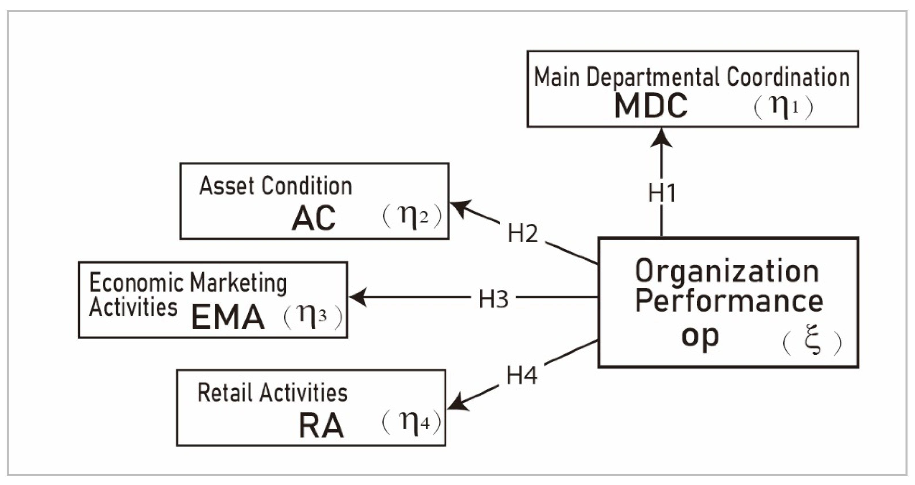
As mentioned earlier, the main departments of LTFAs include promotion, credit, marketing, and insurance. Therefore, the main departmental coordination of the four departments in the organization becomes its core strategy for competitiveness. Therefore, from the perspective of organizational departments, this study examines how the competitiveness of farmers’ associations is reflected by the main departmental coordination and asset condition and allocation. Accordingly, two hypotheses are proposed as follows:
H1. The organization performance of LTFAs can be represented by the main departmental coordination.
H2. The organization performance of LTFAs can be represented by asset condition and allocation.
2.3. Economy Implementation
In the face of increasingly diversified markets and organizational changes over time, the business orientation of LTFAs needs to be adjusted to meet the needs of agricultural development and farmers. Although LTFAs are positioned as social enterprises, they are still responsible for their own profits and losses. In addition to helping promote the government’s agricultural policies, improving the rural economy, and taking care of farmers’ welfare, the operation of their economic business departments plays a pivotal role in the local economy. Subsidies from government departments and project implementation by farmers’ organizations are often seen as affirmative results for organizational competitiveness, and thus this financial assistance from the government will also affect the performance of the economic departments [
38].
In addition, because of their long history and numerous assets, the allocation and revitalization of assets are very important [
6,
18]. In addition, after the COVID-19 pandemic, local consumers’ preferences regarding sales channels and consumption methods of agricultural products have gradually changed from shopping at a wet market to shopping at supermarkets and TFA stores, where they can buy low-temperature products. Therefore, retail channels belonging to TFAs have become an important source of revenue and can meet the needs of TFAs to display and sell agricultural products.
This study proposes the following two hypotheses on whether the competitiveness of TFAs can be demonstrated with two outcomes: business marketing activities and retail activities from a business perspective.
H3. The organization performance of LTFAs can be presented in terms of their economic marketing activities.
H4. The organization performance of LTFAs can be presented in terms of their retail activities.
2.4. Clustering of Local TFAs
Agriculture is the main industry in rural areas. The development of industry, population migration, and the transformation of rural land use have changed the relationship between farmers and the land, which, in turn, has driven the development of organizational models and promoted rural development [
39]. Human behavior is considered one of the direct drivers that influences and changes regional agricultural development, while industrial activity is the endogenous driving force that connects population and land and is the facilitating force for urban–rural development [
39]. The boom in agritourism can lead farmers to adjust their farming activities [
40].
In areas with developed industry and commerce, rural labor outflow is affected by push and pull factors, and rising land prices significantly influence rural development. Thus, the core objective of rural spatial governance is to optimize the structure of rural spatial benefits through equitable distribution while considering the development of all sectors [
39,
41].
The analysis of rural development from the perspective of “population, land, industry” has been widely applied to the classification and spatial governance of rural areas [
39,
42]. Battermann, Deimel and Theuvsen [
15] adopted this viewpoint to analyze the cluster structure of rural areas in Lower Saxony, Germany. The research results support that the clearer the rural classification criteria, the easier the identification of rural clusters, especially for making decisions about economic alternatives in rural areas.
Existing studies on TFAs are mostly divided into different clusters based on geographical location, the urbanization degree of the location, and the level of profitability of the credit department. As they fail to consider the membership structure and industrial conditions of individual TFAs, they are unable to fully reflect the agriculturalization degree in their regions, making it difficult to effectively provide a basis for classification and guidance and creating a problem around financial orientation in policy guidance and competitiveness.
In other words, to demonstrate the physical performance of LTFAs through competitiveness, an appropriate clustering method can help the government develop a feasible strategy for LTFAs in response to the existing operating conditions and resource constraints of each LTFA. Only by clustering LTFAs under different conditions can the importance of each business be adjusted to improve performance.
4. Empirical Results
4.1. Fuzzy C-Means Clustering
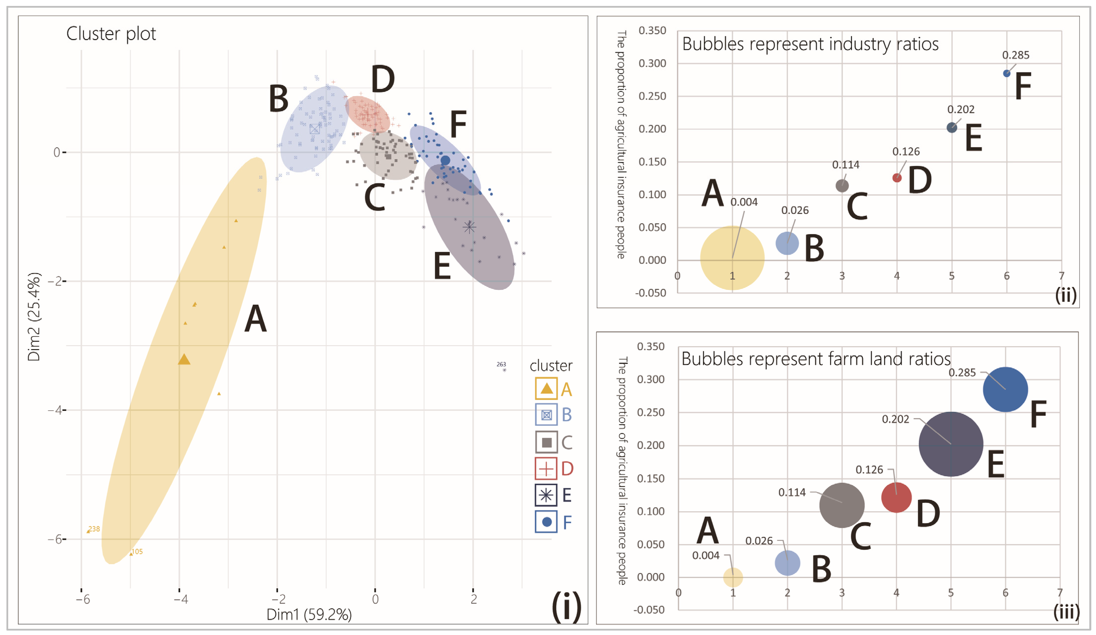
As mentioned earlier, it is difficult to reflect the actual conditions of society and the current times on the basis of existing indicators when classifying the agriculturalization degree in townships and urban areas where LTFAs are located, leading to the dilemma that the analysis results do not fit well with practice. To reflect the conditions of LTFAs in terms of industry and natural resources, this study used the fuzzy C-means (FCM) clustering algorithm to calculate the probability of the distribution of agricultural labor (expressed as the number of people insured by agricultural insurance) and number of industrial and commercial registered households (the non-agriculturalization degree) in each township. We used “agricultural population–agricultural land–industrial activities” as the criterion for clustering. The results were then used to classify LTFAs into six clusters: A, B, C, D, E, and F (
Figure 2i).
To illustrate the differences between the subsets and their characteristics, after determining the attributes of the subsets of individual LTFAs in the above manner, the number of insured farmers in the six clusters was taken as the vertical axis. The series of six classifications was taken as the horizontal axis. The size of the bubble was used to represent the ratio of industry and commerce in the area corresponding to the classification. The larger the bubble, the higher the degree of non-agriculturalization in the area. It can be seen that the industrialization degree in Clusters A and B near the vertical axis is much higher than that in the other groups, indicating that these two clusters are quite urbanized, where Cluster A belongs to the metropolitan area, and the number of farmers and agricultural land resources is not high (
Figure 2ii). Clusters C and D are close to each other in terms of the number of insured farmers, but Cluster C has a higher industrialization degree than Cluster D. Cluster F, on the other hand, has a significantly higher proportion of insured farmers than the other clusters, which also indicates a fairly significant agriculturalization degree.
When considering the resource conditions of agricultural operations and replacing the proportion of industrial and commercial sectors with the proportion of agricultural land in the region, it is clear that Clusters C and E seem to have more favorable conditions for agricultural operations than Clusters D and F. This clearly divides the different clusters (
Figure 2iii). The FCM results veritably provide a clear distinction over the previous classification basis, effectively and clearly clustering the 279 LFAs into six subsets to facilitate subsequent analysis.
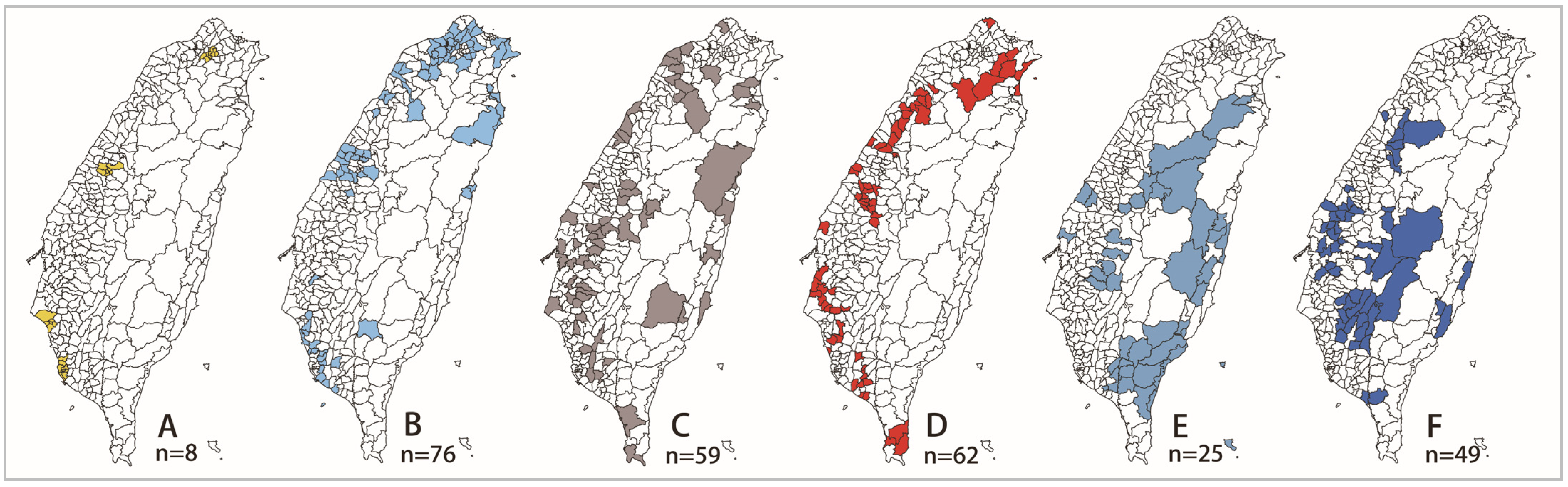
According to the classification of practical organizations based on the six clusters, the two clusters near the left, A and B, are deeply influenced by industrial and commercial development, as they contain a very high proportion of the industrial and commercial sectors but a low proportion of the farming population. Thus, they are named as follows: Cluster A is the urban farming group, and Cluster B is the suburban farming group, indicating that the agricultural business of the area is set for consumption and environmental leisure, respectively. Clusters E and F on the right have the larger agricultural area and a higher proportion of insured farmers. They can be defined as traditional agricultural areas and belong to the farming cluster. There is a clear overlap between the two clusters, indicating that several TFAs may meet their respective conditions in terms of subcluster indicators. Clusters C and D, on the other hand, are between the urban farming cluster and the crop farming cluster and can be defined as the transition farming clusters. Cluster C has more agricultural land resources but a lower proportion of insured farmers, whereas Cluster D has fewer agricultural land resources but a higher proportion of insured farmers. The spatial distribution of the six subsets can be represented in
Figure 3.
4.2. Assessment of the Measurement Model
In the PLS-SEM model, the reliability of the measurement model is assessed as indicator reliability and construct reliability [
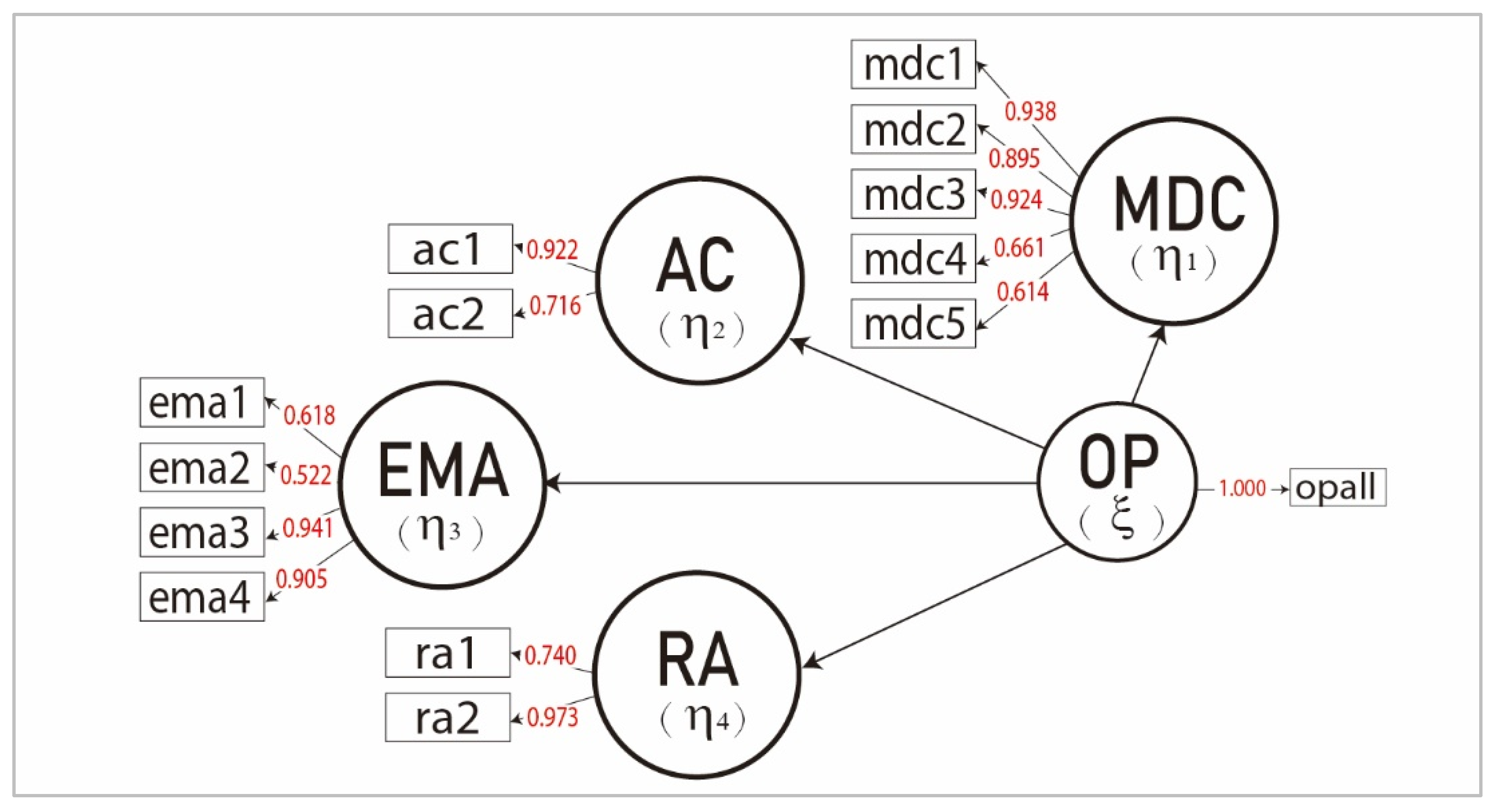
59]. To examine the explanatory power of factors, the standardized factor loading (SFL) of each observed variable needs to be higher than 0.4 and generally reach a threshold value of no less than 0.7. The SFL values of all the observed variables in this study ranged from 0.522 to 0.973 [
54], which are in accordance with the indicator reliability, as shown in
Figure 4. The composite reliability (CR) values of the variables measured in the model ranged from 0.853 to 0.908, and were all higher than the threshold value of 0.7 [
60]. Therefore, the internal consistency reliability is confirmed (
Table 2). The results indicate that the average variance extracted (AVE) values that range from 0.590 to 0.748 for all observed variables are above the recommended threshold of 0.5, indicating that the model has convergent validity.
The discriminant validity was assessed by the Fornell–Larcker criterion, and the square root of the AVE of the target variable was compared with the correlation coefficient of the latent variables. The results indicated that the square root of the AVE of individual components was higher than the correlation coefficient values of other latent variables [
59,
60], indicating that the model in this study has discriminant validity (
Table 3). Then, by using the Heterotrait–Monotrait ratio (HTMT) of correlations proposed through the Monte Carlo simulation, the four conformational values were found to be between 0.348 and 0.792, which were in accordance with the recommendation that the check threshold value needed to be less than 0.85, and thus passed the discriminant validity.
4.3. Assessment of the Structural Model
The hypothesis test of path coefficients of the PLS model can be realized by assessing model fitness through the bootstrap resampling procedure. In this study, after bootstrapping 10,000 times, the path analysis indicates that all four hypotheses are significantly valid in
Table 4. The results clearly support that the main departmental coordination positively influences OP (H1: γ = 0.736), the economic asset condition positively influences OP (H2: γ = 0.476), and economic marketing activities positively influence OP (H3: γ = 0.653). The study on retail activities (H4: γ = 0.465,) also confirms their positive influence on OP, whereas for the competitiveness, it is mainly represented by the quality of the main departmental coordination (MDC), followed by economic marketing activities (EMA). Although retail activities (RA) are important, an unsatisfactory channel sales performance does not mean that a given TFA is less competitive.
4.4. Result of Clustering
This study endeavored to understand the response of LTFAs with different resource conditions in terms of their OP and departmental performance. The study classified 279 LTFAs into six clusters using the classification of “agricultural population–farming land–industrial activities,” which separated 8 LTFAs into Cluster A. Due to an insufficient sample size, the paths of 76 LFTAs in Cluster B, 59 in Cluster C, 62 in Cluster D, 25 in Cluster E, and 49 in Cluster F were examined. The path coefficients (γ) of each cluster were estimated separately. The results are shown in
Table 5 and
Figure 5.
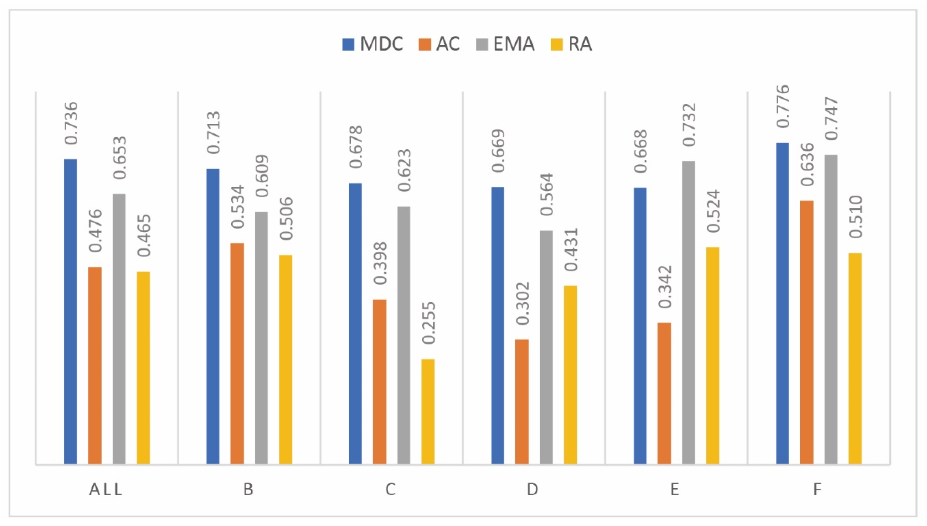
All four hypotheses in Cluster B were valid, with the highest path values for departmental coordination ( = 0.713) and economic marketing activities ( = 0.609), and the explanatory power of departmental coordination is 50%. All four hypotheses in Cluster C were valid, with the highest path values for departmental coordination ( = 0.678) and economic marketing activities ( = 0.623), but retail activities were significant only at the 10% level. Cluster D had the highest path value for economic marketing activities ( = 0.732) and the second highest for departmental coordination ( = 0.669). The hypothesis of the economic asset condition does not hold. In Cluster E, the highest path values were for departmental coordination ( = 0.776) and economic marketing activities ( = 0.732). Hypothesis 2 on the relationship between organization performance (OP) and asset condition (AC) was rejected.
All four hypotheses in Cluster F were valid, with the highest path values for departmental coordination ( = 0.777) and economic marketing activities ( = 0.747), and the explanatory power of departmental coordination was 60%.
To understand the relative degree of the four main facets affected by competitiveness in different groups,
Figure 5 shows the structure coefficients of OP for the four facets of the five groups of LTFAs. Results from all LTFAs (ALL) show that MDC (0.736) and EMA (0.653) were more significantly affected by OP than AC (0.476) and RA (0.465). The figure shows that there was a highly positive relationship between the competitiveness of farmers’ associations that is represented by 11 performance indicators, the functional income of all departments, and the operating income of economic undertakings, whereas its relationship to economic asset conditions and entity sales channel revenue was weaker.
If we examine the structure coefficients of the individual facets of the five groups, it can be seen that except for in Cluster E, OP had a higher influence on EMA than MDC; in the other four groups, OP had a significant influence on MDC and EMA, and MDC was greater than EMA. This shows that OP is reflected in the functional performance of all departments. When OP is improved, it will result in the progress of department services, including financial, insurance, and agricultural extension services. As Cluster E belongs to a traditional farming area with characteristic agricultural products, the operation of economic business departments that provide processing and storage services often play a key function in a region; thus, EMA is an important aspect representing the competitiveness of LTFAs in the group.
In addition, the impact of OP on RA in Clusters D and E was higher than that of AC, which is obviously different from the other three groups. The results show that compared with other groups, OP had a close relationship with marketing and sales services in Clusters D and E. Overall, Cluster F had the highest total value of structure coefficients. Except for RA (0.510), where its value was slightly lower than that of Cluster E, Cluster F’s MDC, EMA, and AC were all higher than those of other groups, indicating that through the corresponding value of organizational performance, this group can effectively show good results for LTFAs in sectoral functions, economic performance, and economic asset conditions. In addition, for Cluster C, the improvement of OP was limited in helping improve marketing and sales; additionally, for Cluster D it can be seen that there is room for improvement in the use of economic assets. Relevant results can provide reference for the decision makers when adjusting resource allocation or planning competitive business policies.
5. Discussion
A hypothesis model was developed to understand the relationship between LTFAs’ OP and the main departmental coordination of their business operations. The results of the study confirmed that the organization performance (OP) of LTFAs is represented by their main departmental coordination (MDC) and is directly and significantly related to their economic asset condition (AC), economic marketing activities (EMA), and retail activities (RA). In other words, the results also indicated that the OP established by the research team can effectively identify and clearly reflect the relative performance differences among LTFAs and help them to establish their own business policy to implement various economic and social goals. Our results are consistent with those previously published in the literature.
The first contribution of this study is the categorization of the separated departmental services of LFTAs into four business constructs. The OP of LTFAs has been shown to consist of two major categories, business and finance, which demonstrates the ability and role of LTFAs in providing farmers with rural and agricultural services as social enterprises through economic undertakings. Each LTFA can understand and master the key points of OP based on 11 indicators, which are conducive to the subsequent adjustment and learning in regard to their business policy.
Another contribution of this study is the classification of “agricultural population–farming land–industrial activity,” which helped divide the 279 LTFAs into six clusters. Cluster B was more influenced by industrial and commercial development, whereas Cluster F had the largest agricultural population ratio (>28.5%) and had the highest explanatory power in terms of OP and the functions of each department. Cluster C had fewer industrial activities than Cluster B and a smaller agricultural population than Cluster D.
Considering that farmers’ associations have the attributes of social enterprises, the public sector can refer to the classification basis of this study and provide financial subsidies or sales assistance to those who are relatively lacking according to the conditions of farmers’ associations. Farmers’ associations can adjust their organizational business policies and the allocation of manpower and resources in various service departments according to their own individual business advantages and organizational competitiveness to effectively meet local needs.
The objective clustering condition of “agricultural population–farming land–industrial activity” revealed that the business orientation of LTFAs in different subsets presents various competitive responses and performance levels under different environmental conditions.
The influence of the physical sales channels of TFA stores and supermarkets was relatively small, which means that the consumption habits related to market shopping need more analysis and attention. In terms of economic marketing activities, the indicators for Clusters B and D indicated that government-subsidized project plans are more important than the net value of machinery. This can probably be explained by the small amount of agricultural land and the small number of people working in agriculture, as well as by the business model that operates better with plans than it does with machinery. There will be a total of 790,000 hectares of farmland in Taiwan in 2021. Among the six groups of LTFAs, the ratio of arable land area to the national area will range from 0.09% to 0.94% on average. Cluster E had the largest area of agricultural land (>1%) among all the subsets, but the agricultural population ratio was lower than that of Cluster F. The assumption of economic AC was not valid, indicating that the competitiveness of such TFAs should be more prudent if the AC is adopted. The OP indicator objectively describes the current year’s status, grasps the differences in various indicators between OP and the natural conditions of the same group of LTFAs, and identifies the strengths through subindicators to break through operational constraints in order to have a positive influence on future operations. A complete business strategy and stable business policies are essential for not-for-profit organizations. There is no best business model, but there is a most suitable business model.
6. Conclusions
This study demonstrated that sustainable competitiveness reflects the operation and financial performance of social enterprise with diversified portfolios. By considering the data of 279 Taiwanese local farmers associations, this context examined organization competitiveness by considering their main departmental coordination, economic asset condition, economic marketing activities, and retail activities. The FCM method was conducted with regional consideration to classify the organization into six clusters with industrial development, population migration and farmland transfer as indicators.
This study results verified that the clusters established an effective classification basis to facilitating financial assistance for government. Moreover, departmental business reflects that organizational competitiveness was expected to serve the decision maker of LTFAs as a reference for adjusting the staffing and funding allocation of various services. Evidently, the complex and multivariate data from annual yearbook was effective measured and established by the FCM.
The empirical results of this paper successfully established that competitiveness indeed is related to its own operating and financial conditions and provides a diversified response to business policies. According to the results, concerns about the departmental services are crucial to the competitiveness. Therefore, considerations of the stakeholder response and cross-year comparisons should be adopted for analysis from a performance aspect.


