1. Introduction
Price volatility is one of the major risks in agricultural markets. Volatile commodity prices may increase policy uncertainty, expose smallholder farmers to higher risks, alter land use, worsen the forecast accuracy of future supply and demand of agricultural commodities, and increase speculative activity in agricultural production [
1]. Therefore, considerable attention has been paid to understanding price volatility in an agricultural context [
2]. One strand of such in the literature has examined the factors that contribute to price volatility in agricultural commodities [
3,
4]. The most discussed are the effects of domestic market conditions, which include: (1) supply shortage due to changing weather conditions, (2) strong growth in domestic demand, (3) surge in energy prices, and (4) implementation of government policy [
5,
6,
7,
8].
While the extensive literature has considered the supply and demand conditions in the domestic market as a potential factor contributing to the volatile agricultural price [
9,
10], the importance of the trade situation has been relatively neglected. Given the surge in trading volumes of agricultural products during the last several decades, the trade volume of agricultural products may contribute to the volatility in prices [
11]. Thus, it is important to examine the agricultural price volatility in the context of international trade. Nevertheless, only a few attempts have yet been made to analyze the importance of trade conditions in explaining agricultural price volatility, to the best of our knowledge [
12,
13,
14,
15]. Most of these studies mainly focus on the impact of levies-related trade policies on price fluctuations [
13,
14,
15], rather than trade volumes. Therefore, we attempt to measure the effects of factors on agricultural price volatility, taking into account the trade volume.
Our model builds upon Armed and Bernard’s [
16] framework to analyze the factors that contribute to price volatility in the agricultural market. Our model differs from the original one in that we consider not only the domestic market conditions but also trade volumes as possible sources of price volatility.Specifically, we assume that the equilibrium price is determined by the structural equation representing the correlation between the amount of production, consumption, export, and import. Furthermore, considering that the existing models are highly dependent on the price elasticity of supply and demand, we also conduct a numerical simulation based on the price elasticity to generalize our results.
We studied the vegetable market in South Korea for empirical analysis. The Korean market provides a suitable setting for our investigation, since the country has nationally promoted a vegetable price stabilization policy to stabilize vegetable prices [
17]. Thus, in this study, we examine the factors that affect the price volatility of vegetable crops in South Korea with a particular focus on the effects of trade situations. Five main vegetables (cabbage, radish, dried red pepper, garlic, and onion) were selected as research objects because they are subject to higher risks and are the main targets of the government price stabilization policy in Korea.
Our contributions are two-fold. First, we expand the literature by exploring the effect of trade conditions on price volatility in the agricultural market. Second, our findings can bring implications for the vegetable price stabilization policy.
The remaining sections are organized as follows:
Section 2 introduces a brief overview of the Korean vegetable market background,
Section 3 proposes the model,
Section 4 describes the data,
Section 5 presents the results, and
Section 6 discusses the conclusion.
2. Vegetable Production and Price Fluctuations in South Korea
Price volatility in agricultural commodities is a major issue in South Korea, and it has been pronounced in the vegetable market. Due to the weather-sensitive and cyclical nature of vegetable production, vegetable crops have been characterized by relatively high price volatility [
18].In response, the South Korean government has established and implemented several treasury support programs since the 1970s to control the vegetable market situation, including (1) a price stabilization system, (2) a production contract, and (3) a reserve program [
19,
20]. Among them, the vegetable price stabilization, enacted in 2017, is the latest policy change to stabilize vegetable prices and support farm households [
21]. The main elements of the price stabilization program are as follows: the program is targeted at seven major field crops—cabbage, radish, garlic, onion, red pepper, green onion, and potato. Among them, cabbage, radish, dried red pepper, garlic, and onion were set as the five main targets from 2018, while green onion and potato were expanded until 2020. For each crop, crisis-control manuals are constructed and mandated to help agricultural producers and stakeholders respond to various risks, such as yield variability [
19]. For example, if the price falls below a threshold, farmers are subject to a partial price subsidy that guarantees 80% of the wholesale price in a normal year. Moreover, if the price drops extremely, mandates are imposed on farmers to manage excess supply, which includes: (1) export, (2) stockpiling, and (3) disposing of the oversupply.
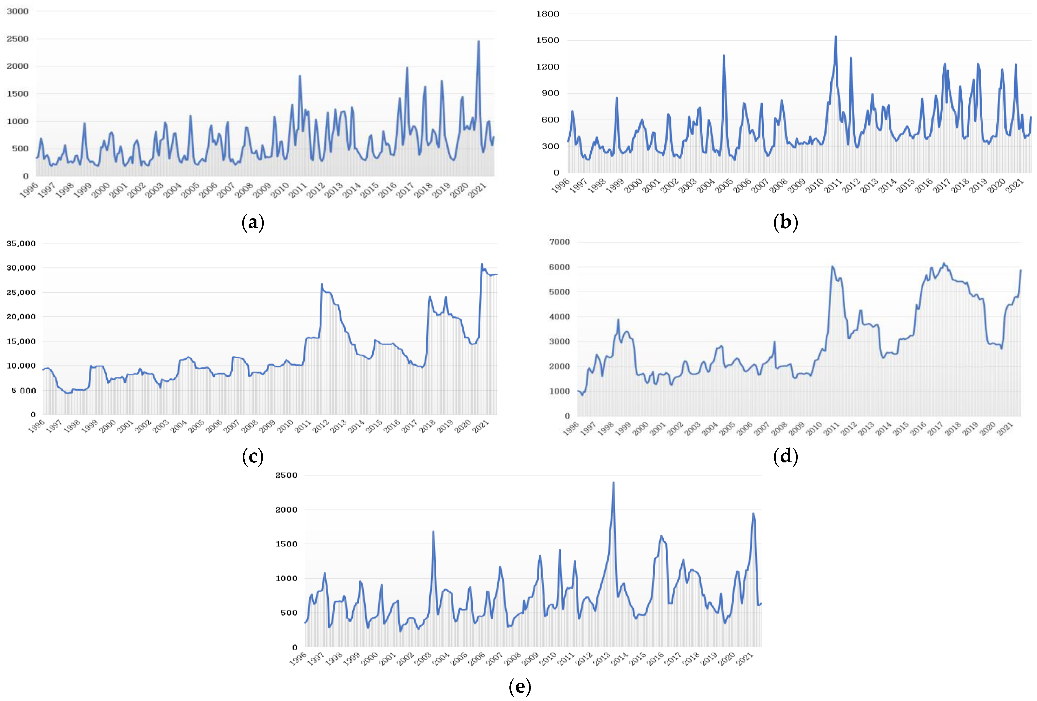
Despite policy efforts, price fluctuations in the vegetable market persist in South Korea. As shown in
Figure 1, which plots the monthly wholesale prices of five major vegetable crops in South Korea—cabbage, radish, dried red pepper, garlic and onion—from 1996 to 2020. Overall, all vegetable crops have witnessed an upward trend in wholesale prices. Furthermore, the magnitude of fluctuation in price series has been enlarged during the last decade. There has been a modest increase in the price series of cabbage and radish, and their seasonal pattern has become more extreme over the last decade. Moreover, there has been a stronger increase in prices for dried red pepper and garlic. Onion has observed a large deviation in price movements during the last decade, contrary to the past trend. Thus, it has been pointed out that the present policy should be evaluated and corrective plans should be established. Hence, revisiting the factors influencing price volatility in the vegetable market has been highlighted.
Figure 2 shows the annual production of five major vegetable crops in South Korea from 1990 to 2020. We presented the detailed trends of yields for cabbage and radish with respect to the harvesting season. Cabbage is classified into four types: namely, Spring Cabbage (harvested between May and June), Highland Cabbage (harvested between July and October), Fall Cabbage (harvested between November and December), and Winter Cabbage (harvested between January and May). Radishes are divided into four types: Spring Radish (harvested between June and July), Highland Radish (harvested between August and October), Fall Radish (harvested between November and December), and Winter Radish (harvested between January and May). From the figure, the annual production of onion has increased over time, while that of dried red peppers and garlic has gradually declined. Cabbage and radish have shown decreasing production trends, except for the slight temporary increase in yields for Spring Cabbage and Spring Radish during the early 2000s.
We examined the correlation between vegetable price volatility (measured by variance) and its production in the following year.
Table 1 represents the result of the correlation analysis. The result revealed an inverse relationship between the two factors, except for onion. The magnitude of correlation is the largest in dried red pepper (−0.27), followed by garlic (−0.26), cabbage (−0.25), and radish (−0.17). The negative relationship between these two values implies that an increase in vegetable price volatility results in a decrease in production in the following year. This can be attributed to farmers’ risk aversion, as they may take measures to mitigate their exposure to price risk, such as reducing production.
3. Methodology
3.1. A Price Fluctuation Analysis Model
In order to examine the factors affecting vegetable price fluctuations in Korea, this paper establishes a new structural model based on the price fluctuation analysis model of Armed and Bernard [
19]. This model was first used by Piggott [
22] and subsequently improved by Myers and Runge [
23]. However, unlike the model of Armed and Bernard, the present study considers the factors that affect vegetable price fluctuations as four factors, including demand, production, imports and exports. Specifically, our model assumes that the equilibrium price of the vegetable market is determined by the structural equations consisting of demand, production, import, and export functions and the market equilibrium equation. In addition, it is assumed that imports and exports are determined exogenously in the structural model (we have attempted to fit equations of imports and exports on price, respectively, for each vegetable, but the results show no significant relations).
Our structural model is specified as follows:
where
denotes vegetable demand,
denotes vegetable supply and
is the vegetable price.
and
denote import and export.
,
,
and
are the demand intercept, supply intercept, import intercept, and supply intercept, respectively (all exogenous demand and supply shift variables, such as agricultural product futures prices, etc., are reduced to net intercept terms of demand and supply functions in order to reduce data and computational needs). Equation (5) is the market equilibrium equation, where the total supply is the sum of domestic supply (domestic production) and imports, and the total demand is the sum of domestic demand and exports.
and
are the constant slope parameters of the demand and supply equation, which can be rewritten as follows:
where
and
represent the price elasticities of demand and supply, representatively.
is the mean price, and
and
are the mean demand and the mean supply. Thus,
and
can be calculated by using the prior estimated elasticities and mean data of price and quantity [
23].
Equations (1)–(4) can be rearranged as:
The system of Equations (8)–(11) and Equation (5) can be expressed as a matrix as follows:
Let
be the vector of
and
be a vector of net intercepts,
. Equation (12) can be written as
Thus, the variance of
,
, is derived as
The variance of equilibrium price
can finally be calculated as the following Equation (15):
where the variance of price
consists of the variances of
, which are the intercepts of the supply function, the demand function, the import function, and the export function, and their covariances. It implies that the price variance is directly attributable to the demand, supply, import, export and their interactions. In other words,
in Equation (15) represent the direct effects of production, demand, import and export, respectively, and the covariance part can be interpreted as the interaction effects of production, demand, import and export. Thus, the ratio obtained by dividing each variance term of production, demand, import and export by the price variance represents the contribution of each factor to the price fluctuation (notably, since our model is not a structural econometric model, it is difficult to separately estimate the impact of other exogenous variables on price fluctuations or volatility clustering effects such as time series models, for example the GARCH model, which can be regarded as a limitation of our study. In addition, our model is limited in its ability to explore seasonality due to its characteristic features, which can be considered to be another limitation).
3.2. A Numerical Simulation
From the above model, it can be easily identified that the variance of price is directly affected by the demand elasticity and the supply elasticity. Therefore, in order to more accurately grasp the influencing factors of vegetable price fluctuation, we conduct a numerical simulation based on these two parameters. We vary the magnitude of these two important parameters to examine the impact of different factors on price fluctuations. Specifically, we proceed with numerical simulations by appropriately scaling up or scaling down the available price elasticity data that have been widely used.
4. Data
This paper takes Korea as an example and uses the annual production, wholesale price, import and export data to analyze the main influencing factors of vegetable price fluctuation during the past 20 years (2001–2020). As mentioned, we select five main vegetables—cabbage, radish, dried red pepper, garlic and onion—as research objects. Cabbage and radish are analyzed separately by crop type. That is, cabbages are classified into spring cabbage, highland cabbage, fall cabbage, and winter cabbage, and radish is classified into spring radish, highland radish, fall radish, and winter radish. The production data were collected from the Crop Production Survey of Statistic Korea, and the wholesale price data were collected from the KAMIS (Korea Agricultural Marketing Information Service) website [
24] of the Korea Agro-Fisheries and Food Trade Corporation. KAMIS contains agricultural wholesale market information, where all wholesale price information includes prices for two qualities of vegetables: high-grade and middle-grade. The price used in this study is the calculated average of these two qualities of vegetable prices. All vegetable import and export data were collected through the “Korea Customs Service Trade Statistics” website [
25].
Table 2 shows descriptive statistics of the variables used in our model. For production, fall cabbage is the highest, followed by onions, spring cabbage, and winter radish. The average wholesale price is highest in order of dried red pepper, garlic, onion and fall radish. In terms of import volume, dried red peppers are the most imported, and spring cabbage is the least. In terms of export volume, onions with the largest production also have the largest exports, and dried red peppers are hardly exported.
Table 3 provides the supply and demand elasticities of five main vegetables used in this study. All supply and demand elasticities used in this study were obtained from the Korea Agricultural Simulation Model (KASMO) developed by the Korea Rural Economic Institute (KREI) in 2020 (more details about KASMO can be found in Seo et al. [
26]). The KASMO is a simultaneous, non-spatial, partial equilibrium model and it is constructed to be generally used as an official tool for analyzing various policy issues related to agriculture and forecasting future prices of commodities in Korea [
27]. It was first developed in 2008 and has been re-estimated and re-specified every year to reflect changes in the Korean agricultural sector. In particular, the supply and demand elasticities estimated from the KASMO are currently used for the annual outlook of Korean agriculture.
5. Results
This study analyzed the direct and interaction effects of supply (production), demand, import and export of five main Korean vegetables. In order to better grasp the effects in different periods, we analyzed the influencing factors of the vegetable price fluctuation in the last 20 years (2001–2020), the 2010s (2011–2020), and the last 5 years (2016–2020), respectively. The results are presented in
Section 5.1. Afterward, considering those direct and interaction effects directly attributable to demand and supply elasticities, we performed a numerical simulation. By varying the magnitude of the elasticity, we simulated different results in the influence of different factors on price fluctuations. The results are presented in
Section 5.2.
5.1. Price Fluctuation Analysis Results
5.1.1. Cabbage
Table 4 reports the price fluctuation analysis results of cabbage, including the direct and interaction effects of production, demand, import and export on cabbage price fluctuation. The results show that, except for the fall cabbage, the other three types of cabbage price fluctuations of the last 20 years are all characterized by a large positive direct effect and a relatively small negative interaction effect. However, for all four types of cabbage, the direct effects of production, demand, import and export are all greater than the interaction effects in all three periods.
From the results of direct effects, supply variability has the largest contribution to the price fluctuations of all types of cabbage in the last 20 years. In other words, supply variability was the dominant force behind Korean cabbage price volatility, especially fall cabbage. The results also show that fluctuations in supply and demand can explain almost all price variations of cabbage in recent years, since trade fluctuations have very little effect. However, in terms of the influencing factors of cabbage price fluctuations in the past 10 years and the past five years, except for fall cabbage, the effect of supply of other types of cabbage has weakened to a certain extent. The price fluctuations of fall cabbage in the past five years were almost entirely affected by supply variations. Furthermore, our results indicate that price fluctuations of different types of cabbage are affected differently by supply and demand, and these effects vary over time, which is also worthwhile to note.
5.1.2. Radish
Table 5 summarizes the price fluctuation analysis results of four types of radishes. The results show that, except for the winter radish, the other three types of radish price fluctuations of the last 20 years are all characterized by a large positive direct effect and a small negative interaction effect. For all four types of radish, the direct effects of production, demand, import and export are all greater than their interaction effects in all periods.
From the results of direct effects, supply variability has the largest contribution to the price changes of all types of cabbage in the past 20 years. Especially for fall radish and winter radish, the supply variation is found to be able to explain 91.99% and 83.27% of its price fluctuation, respectively. However, the effect of supply changed in the 2010s and the last five years. Surprisingly, the price fluctuations of spring radishes over the last five years have been more affected by demand variations, while in the last 10 and 20 years they have been more affected by supply. Highland radishes were also found with similar results. In addition, the impact of import variation was also found in the price fluctuations of highland cabbage, albeit a small proportion. Moreover, like cabbage, the price fluctuations of different types of radishes are affected by different factors. Such results are helpful for the government to formulate corresponding price stabilization policies.
5.1.3. Dried Red Pepper
Table 6 shows the results of the price fluctuation analysis of dried red pepper, including the direct and interaction effects of supply, demand, import and export on dried red pepper price variation. The results show that, for all three periods, dried red pepper price fluctuation is characterized by a large positive direct effect and a comparably small negative interaction effect. This direct effect is the largest in the period of last 20 years and smallest in the last five years.
From the results of direct effects, demand contributed most to the dried red pepper price variation in three periods, especially in the 2010s. Considering the storability of dried red pepper, it can be said to reflect the characteristics of the market by the result that the main influencing factor of price fluctuations is demand. In addition, compared with the 2010s, the proportion of price fluctuations explained by demand is found to be higher in the past five years. Moreover, it is worth noting that the contribution of import variability to dried red pepper price fluctuations is relatively higher than that of supply. It can be explained by the relatively high import dependence on dried red pepper. In Korea, imports of dried red pepper are higher than domestic production.
5.1.4. Garlic
Table 7 shows the results of the price fluctuation analysis of garlic. The results show that garlic price fluctuations of two periods, the last 20 years and the 2010s, are characterized by a large positive direct effect, and a small positive interaction effect. However, in the last five years, the interaction effect has a negative sign, which indicates that the negative interaction effects of supply, demand, import and export on garlic price variation became larger in recent years.
From the results of direct effects, the contribution of supply variability to the price fluctuation of garlic is largest in all three periods, followed by demand, import and export. This effect of domestic production has increased strongly in recent years. In particular, 94.89% of the direct effects of garlic price fluctuations in the last five years can be explained by factors of domestic production. The price volatility of garlic has increased over the past decade in Korea. Therefore, considering our results, it can be suggested that managing domestic production would be the most effective policy to stabilize garlic prices in Korea.
5.1.5. Onion
Table 8 shows the results of the price fluctuation analysis of onion. Onion price fluctuation of the last 20 years is characterized by a large positive direct effect of demand, domestic production, import and export, and a comparably small negative interaction effect. However, in the 2010s and the last five years, onion price fluctuation is characterized by a large positive direct effect and a small positive interaction effect.
For the direct effects of onion price variation, the results over the last 20 years differ significantly from those in the 2010s and the last five years. In recent years, supply and demand play important roles in price fluctuations, whereas trade plays a smaller role. However, over the last 10 years, especially in the last five years, domestic production has played the most important role and the effect of trade has also slightly increased. This indicates that the explanatory power of domestic production for onion price fluctuation in the last five years has reached 91.8%. Thus, like garlic, in order to stabilize the ever-increasing price fluctuations of onions, it would be more effective for the government to formulate supply-side policies.
5.2. Numerical Simulation Results
We performed numerical simulations based on the demand and supply elasticities of five main vegetables. For each vegetable, we increased and decreased the price elasticity by 10%, 20%, and 30% to examine the change of direct effects of demand, supply, import and export on the price fluctuation. We only compared the simulation results for the last 20 years in this subsection.
Figure 3 presents the simulation results of four types of cabbage. It shows the results of the direct effects of demand, supply, import and export using the existing demand and supply elasticities of cabbage, and the results using the 10%, 20%, and 30% increase and decrease in the price elasticities. For spring cabbage, the direct effect of demand on price fluctuation caused by varying the price elasticity ranges from 33.65% to 35.35%, and the effect of supply ranges from 64.75% to 66.34%. The effects of import and export are small and hardly vary with elasticities. However, for highland cabbage, the direct effect of demand on price fluctuation ranges from 24.86% to 35.86% and the effect of supply ranges from 64.04% to 75.57%. It can be seen that the direct effects of demand and supply vary greatly when price elasticities change. However, the contribution of supply variability to price fluctuations is still higher than that of demand and trade volume. In addition, for fall cabbage and winter cabbage, the change of the simulated elasticity has little effect on the change of the proportion of the influencing factors of price fluctuation. It indicates that supply variability explains more price fluctuations of these two types of cabbage.
Figure 4 presents the simulation results of four types of radish. For spring radish, the direct effect of demand on price fluctuation ranges from 32.27% to 39.1%, and the effect of supply ranges from 60.90% to 67.73%. The effects of import and export are almost close to zero in all simulations. For highland radish, the contribution of supply and demand variabilities to price fluctuations are similar and barely changed in all simulations. In addition, for fall radish, although the direct effects of demand and supply on price fluctuations vary with the change of elasticities, the influence of demand is the largest among the four factors, ranging from 87.96% to 93.32%. For winter radish, supply variability plays the most important role in price fluctuations, ranging from 81.64% to 83.84 in all simulations, which is similar to fall radish.
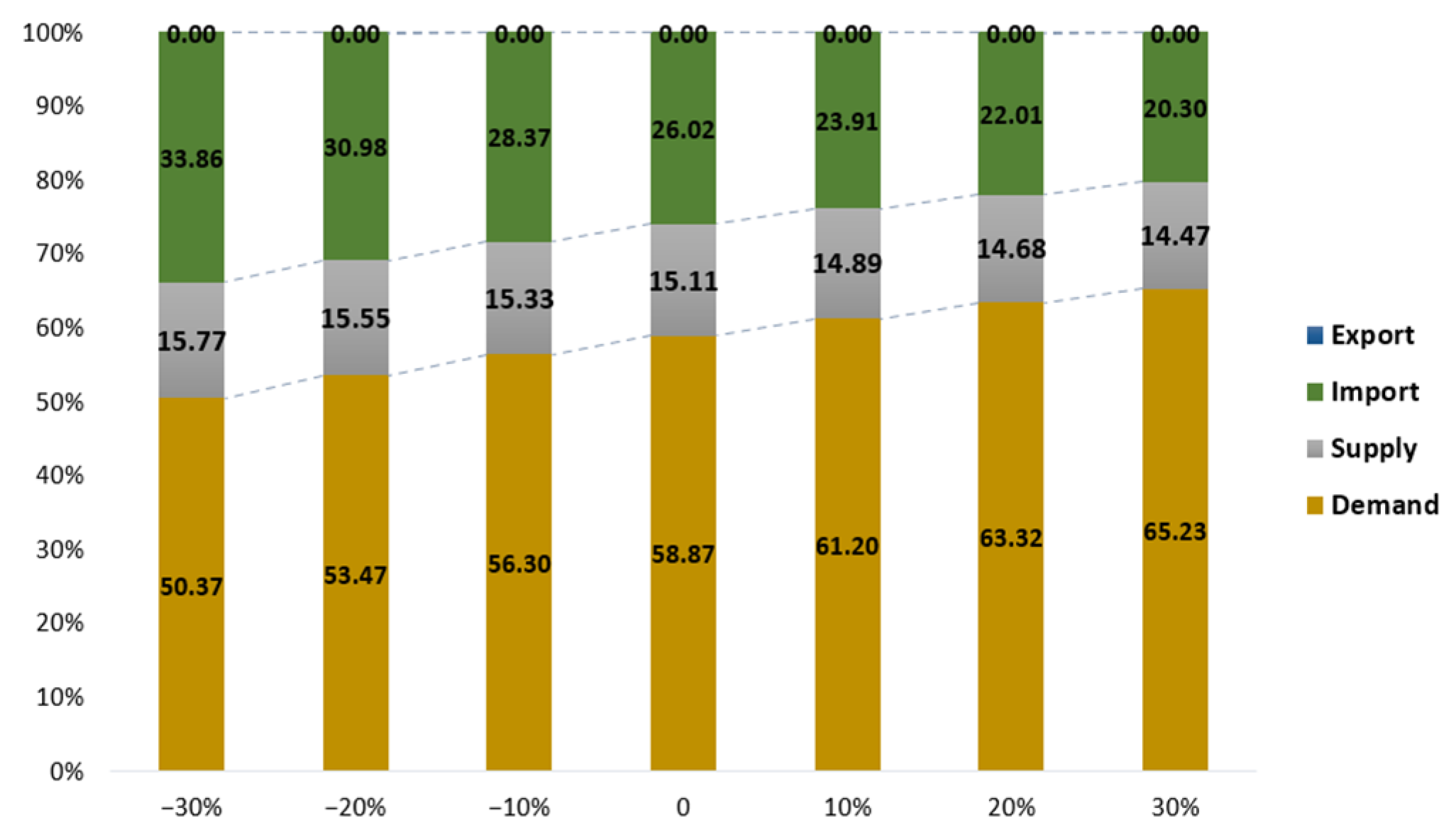
Figure 5 shows the simulation results of dried red pepper. In all simulations, the direct effect of demand on price fluctuation ranges from 50.37% to 65.23%, which is higher than that of the other three factors. It indicates that demand contributed most to the dried red pepper price variation, although price elasticities change. In addition, it should be noted that the contribution of import variation can reach a maximum of 33.86% with the change in price elasticity. Thus, import variation can explain the price fluctuations of dried red pepper better than supply variation.
Figure 6 depicts the simulation results of garlic. The results show that the direct effect of supply on price fluctuation ranges from 82.39% to 87.15%, which is the largest among the four influencing factors. It indicates that supply variability was the dominant force behind the price fluctuations of garlic in the past. Secondly, the contributions of demand and import variation to garlic price fluctuations were found to range from 11.53% to 17.13% and 0.47 to 1.27%, respectively. In addition, the effect of export on price variation is the smallest among all the simulation results.
Figure 7 depicts the simulation results of onion. From these results, the contributions of supply and demand variabilities to price fluctuations are barely changed in all simulations, although demand plays a slightly more important role. In addition, the direct effects of import and export variations on the onion price fluctuation are less than 1%; relatively small.
6. Summary and Conclusions
Price volatility in the vegetable market is a significant global concern. This paper takes South Korea as an example to study the factors affecting price fluctuations of major vegetables—cabbage, radish, dried red pepper, garlic, and onion. We took three time periods, the last 20 years (2001–2020), the 2010s, and the last 5 years, to analyze the effect of demand, supply, import and export factors on the price fluctuations of vegetables in different periods by using a structural price fluctuation analysis model. We further conducted numerical simulations on the elasticity of supply and demand of different vegetables to examine the changes in the factors that affect price fluctuations. Our results are summarized as follows:
First, fluctuations in vegetable prices can be attributed to the direct and interaction effects of demand, supply, import and export, and the direct effect is generally positive and larger than the interaction effect. Second, except for dried red pepper and onion, the direct effect of production fluctuations contributed most to the price fluctuations of vegetables of the last 20 years, while the effects of demand, import and export had relatively low explanatory power regarding price fluctuations. However, for dried red pepper and onion, of which the storage period is, relatively, longer, demand variations play more important roles in price fluctuations than production fluctuations. Specifically, for dried red pepper, import contributed more than production in the last 20 years. Third, compared to the 2010s, except for spring/winter cabbage, spring/winter radish and dried red pepper, the proportion of price fluctuations explained by the production fluctuations of other vegetables was found to have increased in the last five years. This suggests that, in recent years, due to the intensified variation in domestic production, vegetable prices have fluctuated more significantly.
Our results are expected to provide evidential support for the government to formulate policies to stabilize vegetable prices and provide a reference for adjusting the content of existing policies. The following policy recommendations can be drawn in light of our findings. First, in stabilizing vegetable prices, it is relatively efficient to formulate supply-side policies. In specific, it is suggested to formulate a manual on yield and production area to monitor and regulate production accordingly. Second, since there are differences in the characteristics of different vegetables, and the contributions of the influencing factors of price fluctuations are also different, different production management is required for different vegetables. Especially for crops with obvious seasonal characteristics like cabbage and radish, corresponding policies must be formulated according to the type. Third, it would be more effective to implement parallel measures of import and supply management for dried red pepper to stabilize its prices, since its price fluctuations are greatly affected by import variation.
Author Contributions
Conceptualization, Y.Q.; methodology, Y.Q. and B.-i.A.; formal analysis, Y.Q.; resources, M.K.; writing—original draft preparation, Y.Q. and M.K.; writing—review and editing, Y.Q. and M.K.; supervision, B.-i.A.; project administration, B.-i.A. All authors have read and agreed to the published version of the manuscript.
Funding
This research received no external funding.
Institutional Review Board Statement
Not applicable.
Data Availability Statement
The data presented in this study are available on request from the corresponding author.
Conflicts of Interest
The authors declare no conflict of interest.
References
- Gardebroek, C.; Hernandez, M.A. Do energy prices stimulate food price volatility? Examining volatility transmission between US oil, ethanol and corn markets. Energy Econ. 2013, 40, 119–129. [Google Scholar] [CrossRef] [Green Version]
- Mitra, S.; Boussard, J.M. A simple model of endogenous agricultural commodity price fluctuations with storage. Agric. Econ. 2012, 43, 1–15. [Google Scholar] [CrossRef]
- Qu, G.; Lou, Y.; Wu, S.; Deng, X.; Feng, J. Impact of Novel Coronavirus Pneumonia on Agricultural Products Prices: A Case Study of Chengdu. Agriculture 2022, 12, 1688. [Google Scholar] [CrossRef]
- Li, Y.; Zhang, M.; Liu, J.; Su, B.; Lin, X.; Liang, Y.; Bao, Y.; Yang, S.; Zhang, J. Research on the Disturbance Sources of Vegetable Price Fluctuation Based on Grounded Theory and LDA Topic Model. Agriculture 2022, 12, 648. [Google Scholar] [CrossRef]
- McPhail, L.L.; Du, X.; Muhammad, A. Disentangling corn price volatility: The role of global demand, speculation, and energy. J. Agric. Appl. Econ. 2012, 44, 401–410. [Google Scholar] [CrossRef] [Green Version]
- Haniotis, T.; Baffes, J. Placing The 2006/08 Commodity Price Boom into Perspective; Policy Research Working Papers; The World Bank: Washington, DC, USA, 2010. [Google Scholar]
- Kunimitsu, Y.; Sakurai, G.; Iizumi, T. Systemic risk in global agricultural markets and trade liberalization under climate change: Synchronized crop-yield change and agricultural price volatility. Sustainability 2020, 12, 10680. [Google Scholar] [CrossRef]
- Kim, K.S. Decomposition of Factors in Vegetable Price Changes: Changes in Cultivation Area vs. Changes in Yield, NEWMA Form 92; Agrofood New Marketing Research Institute: Los Baños, Philippines, 2015. [Google Scholar]
- Xie, H.; Wang, B. An empirical analysis of the impact of agricultural product price fluctuations on China’s grain yield. Sustainability 2017, 9, 906. [Google Scholar] [CrossRef] [Green Version]
- Rezitis, A.N.; Pachis, D.N. Investigating the price volatility transmission mechanisms of selected fresh vegetable chains in Greece. J. Agribusiness Dev. Emerg. Econ. 2020, 10, 587–611. [Google Scholar] [CrossRef]
- Anderson, K.; Nelgen, S. Trade barrier volatility and agricultural price stabilization. World Dev. 2012, 40, 36–48. [Google Scholar] [CrossRef]
- Loginova, D.; Portmann, M.; Huber, M. Assessing the Effects of Seasonal Tariff-rate Quotas on Vegetable Prices in Switzerland. J. Agric. Econ. 2021, 72, 607–627. [Google Scholar] [CrossRef]
- Yan, W.; Cai, Y.; Lin, F.; Ambaw, D.T. The Impacts of Trade Restrictions on World Agricultural Price Volatility during the COVID-19 Pandemic. China World Econ. 2021, 29, 139–158. [Google Scholar] [CrossRef]
- Berger, J.; Dalheimer, B.; Brümmer, B. Effects of Variable EU Import Levies on Corn Price Volatility. Food Policy 2021, 101, 102063. [Google Scholar] [CrossRef]
- Sun, T.T.; Su, C.W.; Mirza, N.; Umar, M. How does trade policy uncertainty affect agriculture commodity prices? Pac.-Basin Financ. J. 2021, 66, 101514. [Google Scholar] [CrossRef]
- Ahmed, R.; Bernard, A. Rice Price Fluctuation and an Approach to Price Stabilization in Bangladesh; The International Food Policy Research Institute: Washington, DC, USA, 1989; pp. 35–36. [Google Scholar]
- Moon, H.P.; Kim, K.P.; Eo, M.G.; Lee, J.Y. Factors Influencing the Export of Agricultural Products and Effects of Export Support Programs in Korea. J. Rural Dev. 2012, 35, 69–90. [Google Scholar]
- Stulec, I.; Petljak, K.; Bakovic, T. Effectiveness of weather derivatives as a hedge against the weather risk in agriculture. Agric. Econ. 2016, 62, 356–362. [Google Scholar] [CrossRef] [Green Version]
- Kim, W.T.; Han, E.S.; Shin, S.C.; Kook, S.Y.; Seo, H.S. A Study on Calculating the Standard Supply and Demand Quantity for Efficient Operation of the Vegetable Price Stabilization Policy; Korea Rural Economic Institute: Naju, Republic of Korea, 2020; Available online: https://repository.krei.re.kr/bitstream/2018.oak/26461/1/P267.pdf (accessed on 5 August 2022). (In Korean)
- Choi, B.O. A Study on Efficiency Improvement of Nozig Vegetable Supply and Demand Stabilization Project; Korea Rural Economic Institute: Naju, Republic of Korea, 2013. (In Korean) [Google Scholar]
- Ryu, S.; Han, S.; Jang, H.; Kim, D. Improvement plan for vegetables by introducing the production and shipment stabilization policy. Korean J. Agric. Sci. 2019, 46, 813–825. [Google Scholar]
- Piggott, R.R. Decomposing the variance of gross revenue into demand and supply components. Aust. J. Agric. Econ. 1978, 22, 145–157. [Google Scholar] [CrossRef] [Green Version]
- Myers, R.J.; Runge, C.F. The relative contribution of Supply and demand to instability in the US corn market. North Cent. J. Agric. Econ. 1985, 7, 70–78. [Google Scholar]
- Korea Agro-Fisheries & Food Trade Corporation. Korea Agricultural Marketing Information Service (KAMIS). Available online: https://www.kamis.or.kr/customer/main/main.do (accessed on 5 August 2022).
- Korea Customs Service. Korea Customs Service Trade Statistics Website. Available online: https://unipass.customs.go.kr/ets/index_eng.do (accessed on 5 August 2022).
- Seo, H.; Kim, C.; Kim, J. A Study on Development of Korea Agricultural Outlook Model, KREI-KASMO 2020; Korea Rural Economic Institute: Naju, Republic of Korea, 2021. [Google Scholar]
- Han, S.H.; Lee, D.S. Impacts of the Korea-US FTA: Application of the Korea agricultural simulation model. J. Int. Agric. Trade Dev. 2010, 1556, 41. [Google Scholar]
| Disclaimer/Publisher’s Note: The statements, opinions and data contained in all publications are solely those of the individual author(s) and contributor(s) and not of MDPI and/or the editor(s). MDPI and/or the editor(s) disclaim responsibility for any injury to people or property resulting from any ideas, methods, instructions or products referred to in the content. |
© 2023 by the authors. Licensee MDPI, Basel, Switzerland. This article is an open access article distributed under the terms and conditions of the Creative Commons Attribution (CC BY) license (https://creativecommons.org/licenses/by/4.0/).


