Multi-Granularity Feature Aggregation with Self-Attention and Spatial Reasoning for Fine-Grained Crop Disease Classification

Abstract

Combining disease categories and crop species leads to complex intra-class and inter-class differences. Significant intra-class difference and subtle inter-class difference pose a great challenge to high-precision crop disease classification tasks. To this end, we propose a multi-granularity feature aggregation method for accurately identifying disease types and crop species as well as better understanding the disease-affected regions implicitly. Specifically, in order to capture fine-grained discriminating clues to disease categories, we first explored the pixel-level spatial self-attention to model the pair-wise semantic relations. Second, we utilized the block-level channel self-attention to enhance the feature-discriminative ability of different crop species. Finally, we used a spatial reasoning module to model the spatial geometric relationship of the image patches sequentially, such that the feature-discriminative ability of characterizing both diseases and species is further improved. The proposed model was verified on the PDR2018 dataset, the FGVC8 dataset, and the non-lab dataset PlantDoc. Experimental results demonstrated our method reported respective classification accuracies of 88.32%, 89.95%, and 89.75% along with F1-scores of 88.20%, 89.24%, and 89.13% on three datasets. More importantly, the proposed architecture not only improved the classification accuracy but also promised model efficiency with low complexity, which is beneficial for precision agricultural applications.

1. Introduction

Crop disease is one of the major agricultural disasters, and the harmful effect of a wide spread of crop disease usually manifests itself in a significant reduction in crop yield and quality. Previously, farmers and agricultural experts identified crop diseases based on personal experience, suffering limited scope and deteriorating disease identification accuracy. Since there are numerous disease categories and crop types that are influenced by outdoor environments such as light, occlusion, and jitter, different types of crop diseases show significant intra-class differences. However, different subcategories of the same disease have similar disease appearances and can only be discriminated by capturing distinguishing features in subtle regions, which poses a great challenge to high-precision crop disease classification tasks. Therefore, it is critical to design a high-performance crop disease identification model and adopt timely and effective control measures for improving crop yield and quality.

Crop disease is characterized by significant intra-class differences and subtle inter-class differences. Consequently, the crop disease classification problem belongs to the fine-grained classification problem. In the early stage, manual identification methods mainly relied on expert experience to identify crop diseases, which was time-consuming and laborious, and the misdiagnosis rate was high for diseases with a similar appearance. With the development and improvement of computer vision technology, machine learning-based methods and deep learning-based methods have promoted accurate crop disease identification. Machine learning-based methods firstly preprocess the acquired leaf images [1,2,3,4,5], such as denoising, image conversion, and image enhancement. Secondly, the region of interest is segmented from the background. In [6,7,8,9,10,11,12], researchers segmented the crop disease area and background through canny edge detection, Grabcut segmentation, Otsu segmentation, and K-means segmentation methods. Then, features of the region of interest are extracted, which are usually color, texture, and shape features [13,14,15]. Studies have shown that texture features work best for disease identification. In [13], the gray level co-occurrence matrix was used to extract corn disease texture features. In [14], disease texture features are extracted by a spatial grayscale dependency matrix. Pires et al. [15] compared scale-invariant feature transform (SIFT), dense scale-invariant feature transform (DSIFT), pyramid histograms of visual words (PHOW), speeded-up robust features (SURF), histogram of oriented gradients (HOG), and other feature extraction methods, the results showed that the best model performance was achieved by using PHOW to extract soybean disease characteristics. Finally, the extracted features are sent to the classifier for training [16,17,18,19,20]. In [16], three different methods of Patternnet neural network, support vector machine, and k-nearest neighbor (KNN) are used to train the extracted features, and KNN achieves the best results through experiments. [17] utilized SVM and grid search-based SVM to train on the PlantVillage dataset. The SVM classifier model achieved 80% accuracy, and the grid search-based SVM classifier model achieved 84% accuracy. Hlaing et al. [18] used SIFT to extract the texture features of tomato diseases and then sent them to the SVM classifier for training, and achieved an accuracy of 84%. Based on the analysis of the above studies, it could be seen that machine learning-based disease identification methods have major limitations, such as the hyperparameters’ selection in segmentation methods, which can have a large impact on model performance; segmentation is particularly difficult in the complex backgrounds; hand-crafted feature extraction method is less optimized, etc.

In contrast, deep learning-based methods can automatically extract image features, reduce the workload of image segmentation and feature extraction in machine learning methods, and enable end-to-end training. This has led to the widespread application of deep learning-based methods in the field of crop disease classification and has become a research hotspot. Convolutional neural networks (CNN) [21,22,23,24,25,26,27,28,29,30,31,32], a representative algorithm of deep learning, perform the best in crop disease classification. Mohanty et al. [21] trained the PlantVillage dataset using AlexNet [31] and GoogleNet [32] and achieved an accuracy of 99.35%, which validated the feasibility of this method. Ferentinos et al. [22] explored several convolutional neural networks using 25 different types of plants and found that VGG achieved the best performance with an accuracy of 99.53%. Sladojevic et al. [23] proposed a deep convolutional network-based plant disease recognition model that was able to distinguish between healthy leaves and 13 types of diseases with an overall accuracy of 96.3%. Grinblat et al. [24] utilized deep convolution neural networks to classify three bean species and experimentally demonstrated that the accuracy monotonically improved with increasing model depth. Ma et al. [25] proposed a deep convolution neural network to identify cucumber diseases and compared it with traditional classifiers using random forests and support vector machines as well as AlexNet and proved its effectiveness in identifying cucumber diseases in real scenarios. This method achieved 93.4% and 92.2% accuracy on the balanced and unbalanced datasets, respectively. However, a large amount of training data are required for deep convolutional neural networks to achieve excellent performance, for which researchers have used the idea of transfer learning [33,34,35,36] to further improve model classification accuracy using CNN models pre-trained on ImageNet datasets. For example, Kaya et al. [33] studied four different transfer learning methods on four public datasets and experimentally showed that transfer learning models based on fine-tuning are more beneficial in improving model classification performance. Too et al. [34] fine-tuned several state-of-the-art deep CNN models on the PlantVillage dataset and obtained a model with an accuracy of 99.75%. Cruz et al. [35] recognized grape diseases with ResNet50 [37] backbone, obtaining balanced training time and accuracy. Numerous experiments have demonstrated that transfer learning can effectively improve the classification performance of deep convolution networks.

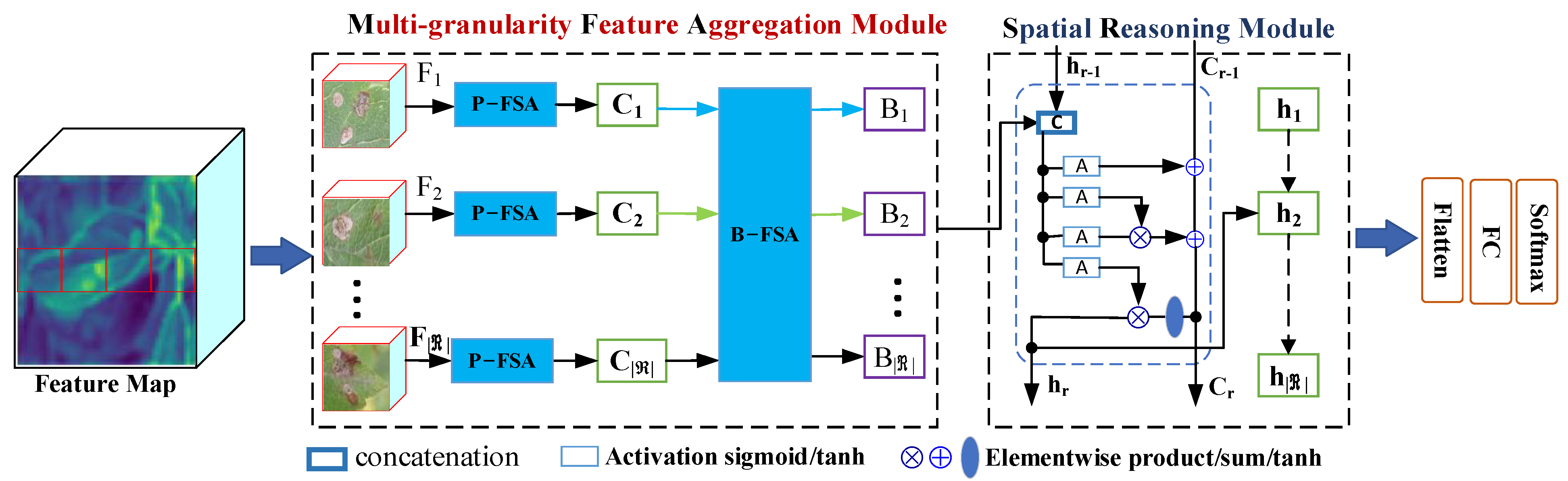
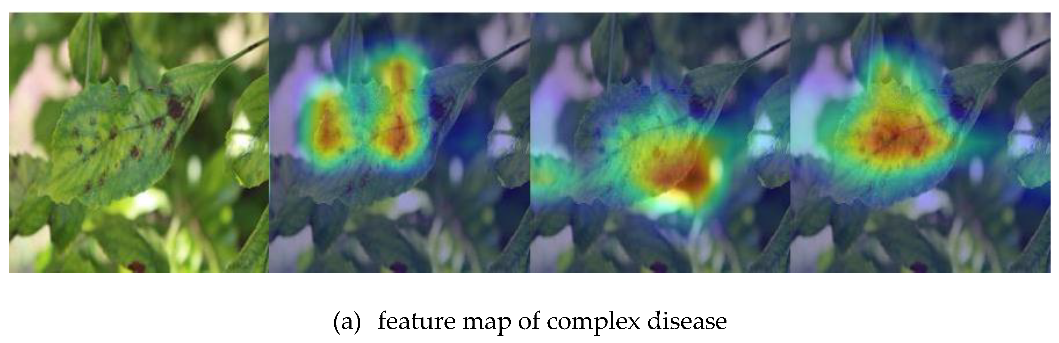
In the above studies, the models can achieve good classification results when the intra-class differences are large. However, the model performance is not satisfactory when the inter-class differences are small. To this end, a multi-granularity feature aggregation method was proposed to better capture discriminative features of subtle regions to differentiate crop diseases with similar appearances. Firstly, we utilized a pre-trained CNN to extract the feature of the input images, which were divided into several non-overlapping patches. Secondly, we explored the pixel-level spatial self-attention module to capture fine-grained discriminative cues for each disease category. Subsequently, we further investigated the block-level coarse-grained channel self-attention module for improving the discrimination of different crop species features. In addition, taking into account that the diseases are randomly distributed over distinct locations of the leaves, we exploited the spatial reasoning module to model the spatial geometric relationships between image blocks sequentially to further enhance the feature representation of the diseases for improving the discriminatory ability of disease and species characteristics. The main contributions of this paper are as follows:

(1)

A multi-granularity feature aggregation method is proposed to strengthen the connection between different granularity features by exploring multiple regions and hierarchically learning the discriminative disease feature from pixel level to block level.

(2)

Considering that subtle changes in the overall region and its spatial arrangement can better refine the learning process, a spatial reasoning module is introduced to improve the model’s performance.

(3)

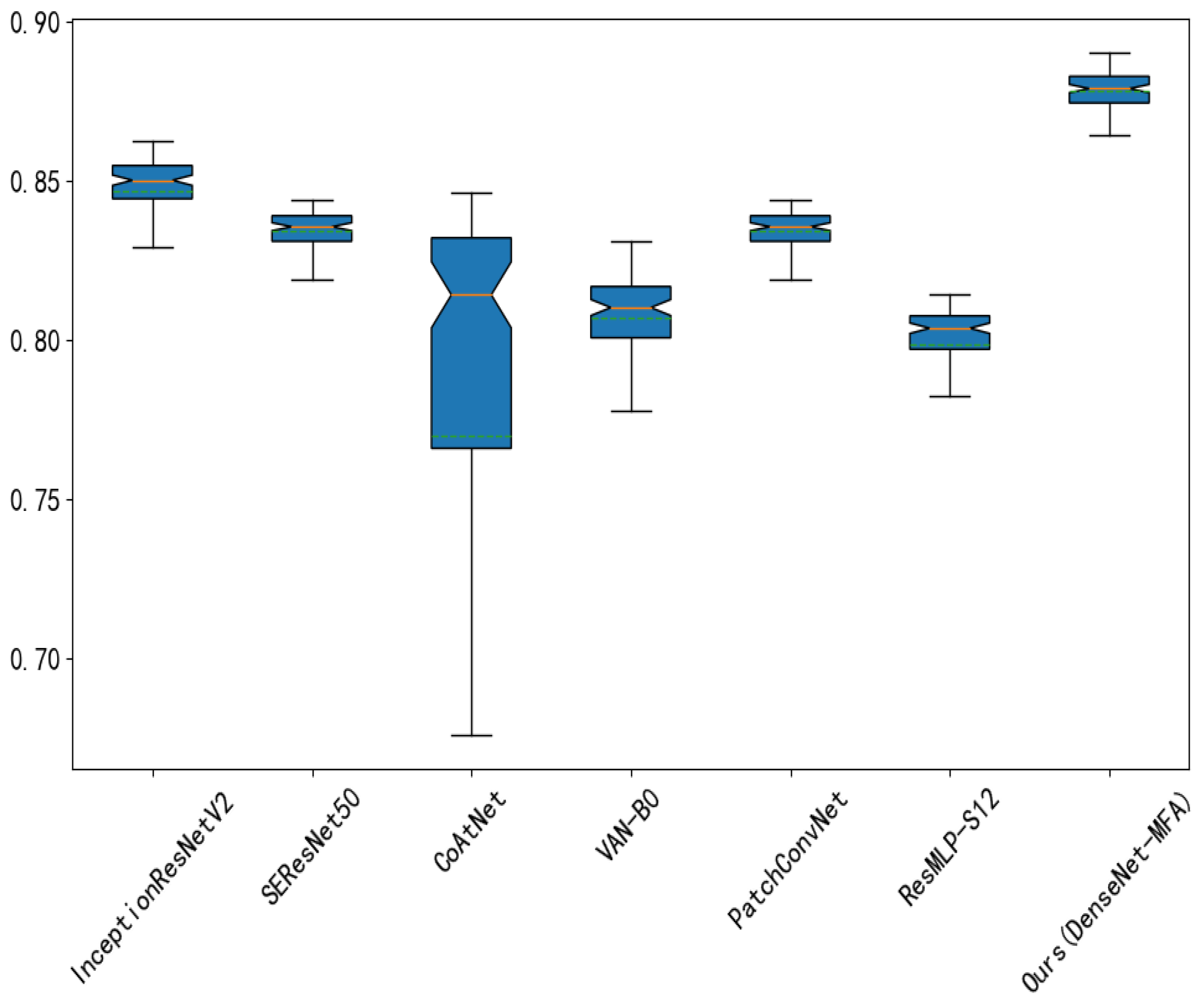
The experimental results of PDR2018, FGVC8 and non-lab PlantDoc datasets show that the method not only effectively improves the classification accuracy, but also has low complexity.

The sections of this paper are organized as follows: In Section 2, the dataset is introduced. Section 3 describes the method proposed in this paper. The experimental results and analysis are given in Section 4. Discussion of the method of this paper is given in Section 5. Conclusions are given in Section 6.

2. Materials

As shown in

Table 1. Overview of the three datasets.

Dataset	Class	Number of Training Sets	Number of Validation Sets
PDR2018	59	31,716	4539
FGVC8	12	14,901	3731
PlantDoc	27	2340	236

, our proposed method was validated on the PDR2018, FGVC8, and PlantDoc datasets. The PDR2018 dataset with 61 disease categories was provided by the AI Challenger 2018 Crop Disease Detection Competition. The dataset was extremely unbalanced in terms of categories, with only 2 and 1 images for diseases in categories 44 and 45, respectively. Hence, these two categories were removed during the experiments. The detailed name of disease types can be found in Guan et al. [38].

The FGVC8 dataset was provided by the Kaggle competition Plant Pathology 2021-FGVC8, and the image size was 4000 × 2672 pixels, taken by high-resolution cameras with different angles, lighting, and backgrounds. Each image had one or more labels indicating leaf disease. The training and validation sets were divided into a ratio of 8:2. The short names of the disease are shown in

Table 2. Abbreviation of the name of disease category on the FGVC8 dataset.

Number	Disease Name	Number	Disease Name
F1	complex	F7	rust
F2	frog eye leaf spot	F8	rust complex
F3	frog eye leaf spot complex	F9	rust frog eye leaf spot
F4	healthy	F10	scab
F5	powdery mildew	F11	scab frog eye leaf spot
F6	powdery mildew complex	F12	scab frog eye leaf spot complex

.

The PlantDoc dataset covered disease images of 13 species in real scenarios with 27 classes. The authors removed inappropriate images such as leafless plants, laboratory-controlled, out-of-scope, and duplicate images. The detailed name of disease types can be found in Singh et al. [39].

As shown in Figure 1, the sample crop disease images of different categories on the three datasets were also provided. It is clear that the images in the PDR2018 dataset have less background interference, but also that the images in the FGVC8 and PlantDoc datasets are much more challenging.

3. The Proposed Method

As shown in Figure 2, the proposed multi-granularity feature fusion network mainly comprised four modules. Firstly, the feature maps $F_B$ of the input images were extracted with a backbone, such as DenseNet121 [40]. Secondly, obtaining processed feature maps $F_{MFA}$ by the multi-granularity feature aggregation module (MFA), which captured both local and global spatial relationships. Thirdly, the sequential spatial reasoning (SSR) module was used to capture the spatial geometry relationships between different feature blocks. Finally, the crop disease identification results were obtained using the classical classification head based on the $F_{SSR}$. Each of the modules will be detailed in the following sections.

3.1. Feature Extraction

In recent years, convolution neural networks have excelled in the field of computer vision, capturing both high-level semantic features in deep layers and low-level spatial features in shallow layers. The ResNet [37] proposed by He et al. solves the network degradation and gradient disappearance problems by utilizing the residual module, which speeds up the network training. DenseNet [40] enhances feature propagation through feature reuse and bypass settings, greatly reducing the number of parameters and making it more efficient than other networks. More recently, MobileNetV2 [41] introduced inverted residuals and a linear bottleneck structure to preserve feature diversity when enhancing gradient propagation and greatly reducing the computation. Motivated by this, all three models mentioned above were evaluated and the best model was selected for subsequent experiments. It was experimentally validated that Densenet121 [40] was slightly better than the other two models. A more detailed description will be provided in the experimental Section 4.3.1.

3.2. Multi-Granularity Feature Aggregation (MFA)

The MFA module was designed to address the problem of high intra-class and low inter-class variability in crop diseases. The output feature map $F_B$ was delivered to the MFA module in order to enhance feature representation with both local and global spatial relationships. Since the resolution of the feature map in the last layer was too low to identify the appearance of the lesion information, the feature map was upsampled to 28 × 28 with bilinear interpolation before feeding into the MFA module.

The proposed MFA module comprised pixel-level feature self-attention (P-FSA) module and block-level feature self-attention (B-FSA) module, as shown in Figure 3. The P-FSA module and B-FSA module were connected to each other.

3.2.1. P-FSA Module

Firstly, as shown in Figure 3, the input feature map was divided into K × K feature blocks, and the feature block set was denoted as ${\left\{F_i\right\}}_{i=1}^{\left|R\right|}$, where $\left|R\right|$ was the total number of blocks. Secondly, each feature block $F_i$ went through the P-FSA module, which captured the pixel-level relationship in each block. The output of each P-FSA module was denoted as ${\left\{C_i\right\}}_{i=1}^{\left|R\right|}$. The detailed architecture of the P-FSA module is depicted in Figure 4.

The P-FSA module we explored could mine and enhance the discriminative features from different disease regions. In this paper, $\left|R\right|=4\times 4=16$. The module captured long-range dependencies by directly calculating the spatial relationship between two locations to implicitly discover the location of the disease area.

3.2.2. B-FSA Module

Different from the P-FSA module, the B-FSA module was utilized to model the long-range relationship among the block-level features. Similarly, all the $\left|R\right|$ blocks were delivered to the B-FSA module as shown in Figure 5, and the output was represented as ${\left\{B_i\right\}}_{i=1}^{\left|R\right|}$. Based on these operations, the MFA module fused both pixel-level and block-level features in this framework.

The B-FSA module we introduced could improve the model’s ability to discriminate the characteristics of different crop species. After the image blocks passed through the pixel-level feature self-attention module, fine-grained discriminative cues of disease classes were captured and a series of feature vectors $C_r$, $r\in \left|R\right|$ were generated. However, there were some similarities in appearance features among the subclasses, which formed subtle inter-class differences that were difficult to distinguish, which was the challenge in fine-grained crop disease classification. In response, we proposed a block-level feature self-attention module that enabled the model to selectively focus on more relevant regions by calculating the similarity between itself and its neighboring environment, and thus extract discriminative features.

3.2.3. FSA Module

The P-FSA module and the B-FSA module utilized the feature self-attention module shown in Figure 6 to capture local discriminative features. It is worth mentioning that all the FSA modules shared the same parameters. It was similar to the classical non-local module, but with a difference in calculating the self-attention matrix with reduced channels for computational efficiency. The flow of the FSA module is described as follows.

(1)

The input feature $X\in {ℝ}^{H\times W\times C}$ used three $1\times 1$ convolutions $W_{\varphi }$,$W_{\theta }$,$W_{\gamma }$, and obtained three features $\varphi \in {ℝ}^{H\times W\times \raisebox{1ex}{$C$}\!\left/ \!\raisebox{-1ex}{$2$}\right.}$, $\theta \in {ℝ}^{H\times W\times \raisebox{1ex}{$C$}\!\left/ \!\raisebox{-1ex}{$2$}\right.}$, $\gamma \in {ℝ}^{H\times W\times C}$.

$$\varphi =W_{\varphi }\left(X\right),\theta =W_{\theta }\left(X\right),\gamma =W_{\gamma }\left(X\right)$$

(1)

(2)

Calculate the similarity matrix $S\in {ℝ}^{\left(H\times W\right)\times \left(H\times W\right)}$.

$$S=\mathrm{transpose}\left(\varphi \right)\times \theta$$

(2)

(3)

Use softmax to normalize the similarity matrix $S$.

$$\overrightarrow{S}=softmax\left(S\right)$$

(3)

(4)

Weighted summation based on the similarity of feature vectors.

$$O=\overrightarrow{S}\times {\gamma }^T$$

(4)

(5)

Use the $1\times 1$ convolution $W_O$ and sum with the input feature, obtain the final output $X^{\prime }\in {ℝ}^{H\times W\times C}$.

$$X^{\prime }=cat\left(W_O\left(O^T\right),X\right)$$

(5)

3.2.4. Sequential Spatial Reasoning (SSR)

As shown in Figure 3, the SSR module captured the spatial geometric relationships of different feature blocks. It could pass useful information learned in the previous moment to help the current moment of learning, and output the desired information after selective filtering. The output was represented as ${\left\{h_i\right\}}_{i=1}^{\left|R\right|}$. The spatial reasoning module we explored was capable of enhancing the global representation of features and further improving the recognition of disease and species features. After the MFA module, the model captured the multi-granularity features and generated the feature vector $B_r$, $r\in \left|R\right|$. The module first decided what information from the previous moment could be passed to the current moment. Then the information was updated based on the output of the previous moment and the current input. Finally, information filtering was performed to get the required information. The specific steps are shown in Equations (6)–(11).

$$f_r=sigmoid\left(W_f·\left[h_{r-1},B_r\right]+{\alpha }_f\right)$$

(6)

$$i_r=sigmoid\left(W_i·\left[h_{r-1},B_r\right]+{\alpha }_i\right)$$

(7)

$$\widetilde{C_r}=tanh\left(W_c·\left[h_{r-1},B_r\right]+{\alpha }_c\right)$$

(8)

$$C_r=f_r\times C_{r-1}+i_r\times \widetilde{C_r}$$

(9)

$$o_r=sigmoid\left(W_o\left[h_{r-1},B_r\right]+{\alpha }_o\right)$$

(10)

$$h_r=o_r\times \tanh \left(C_r\right)$$

(11)

where $B_r$ represents the input of the current moment, $h_{r-1}$ represents the output of the previous moment, $f_r$ determines the useful information at the previous moment, $i_r$ determines the important valid information of the current input, $\widetilde{C_r}$ saves the valid important information,$C_r$ updates the valid important information,$o_r$ determines whether the information from the current moment is added to $h_r$, and $h_r$ represents the final output information. $W_{*}$ are the weight matrices, and ${\alpha }_{*}$ are the biases.

4. Experiments and Results

4.1. Experimental Setting

The experiment was conducted on an Ubuntu 18.04 64-bit system with TensorFlow 1.13 [42]. The input image was uniformly resized to 224 × 224 pixels. The batch size was set to 32, and the network was trained by the SGD optimization method with the initial learning rate of 0.0001 and the momentum with 0.99. Data augmentation methods such as random clipping, random zooming, horizontal flipping, and random rotation were used during the model training.

4.2. Metrics

We adopted accuracy, precision, recall and F1-score as the model performance evaluation metrics in this paper, which are demonstrated in Equations (12)–(15).

$$accuracy=\frac{TP+TN}{TP+TN+FP+FN}$$

(12)

$$Precision=\frac{TP}{TP+FP}$$

(13)

$$Recall=\frac{TP}{TP+FN}$$

(14)

$$\text{F1-score}=2\times \frac{\left(Precision\times Recall\right)}{\left(Precision+Recall\right)}$$

(15)

where TP denotes positive samples with correct classification, FP denotes negative samples misclassified as positives, TN denotes negative samples with correct classification, and FN denotes positive samples misclassified as negatives.

4.3. Ablation Study

4.3.1. Comparison with Different Backbones

In order to select the best performing backbone network, comparison results of ResNet50, MobileNetV2, and DenseNet121 in terms of accuracy, precision, recall, and F1-score are shown in

Table 3. Results of the baseline model on PDR2018, FGVC8, and PlantDoc datasets.

Dataset	Backbone	Accuracy	Precision	Recall	F1-Score
PDR2018	ResNet50	85.37%	85.74%	85.37%	85.55%
	MobileNetV2	83.94%	84.88%	83.94%	84.41%
	DenseNet121	85.59%	86.07%	85.59%	85.83%
FGVC8	ResNet50	86.64%	85.34%	86.64%	85.99%
	MobileNetV2	85.21%	85.13%	85.21%	85.17%
	DenseNet121	87.04%	86.79%	87.04%	86.91%
PlantDoc	ResNet50	85.08%	86.04%	85.08%	85.56%
	MobileNetV2	85.05%	85.54%	85.05%	85.29%
	DenseNet121	86.36%	87.30%	86.36%	86.83%

respectively. It was clear that DenseNet121 achieved the best result on PDR2018, FGVC8, and PlantDoc datasets. More specifically, in terms of accuracy, it improved by 0.22% and 1.65% over ResNet50 and MobileNetV2 for the PDR2018 dataset. Besides, the F1-score of DenseNet121 was about 0.28% and 1.42% higher than ResNet50 and MobileNetV2.

On the FGVC8 dataset, DenseNet121 improved 0.4% and 1.83% over ResNet50 and MobileNetV2 in accuracy, and also 0.92% and 1.74% higher in F1-score respectively.

On the PlantDoc dataset, DenseNet121 improved 1.28% and 1.31% over ResNet50 and MobileNetV2 in accuracy, and also 1.27% and 1.54% higher in F1-score respectively. DenseNet121 was therefore chosen as the baseline backbone for the following experiments.

4.3.2. Comparison between Different Modules

Ablation studies were performed to validate the effectiveness of the proposed module as shown in

Table 4. Ablation studies of different modules on PDR2018 dataset.

	P-FSA	B-FSA	SSR	Accuracy	Precision	Recall	F1-Score
1				85.59%	86.07%	85.59%	85.83%
2	√			85.92%	86.52%	85.92%	86.22%
3		√		85.78%	86.27%	85.78%	86.02%
4			√	85.71%	86.60%	85.71%	86.15%
5	√		√	86.96%	87.01%	86.96%	86.98%
6		√	√	87.01%	87.05%	87.01%	87.03%
7	√	√		87.21%	87.56%	87.21%	87.38%
8	√	√	√	88.32%	88.08%	88.32%	88.20%

,

Table 5. Ablation studies of different modules on FGVC8 dataset.

	P-FSA	B-FSA	SSR	Accuracy	Precision	Recall	F1-Score
1				87.04%	86.79%	87.04%	86.91%
2	√			87.40%	87.09%	87.40%	87.24%
3		√		87.36%	86.98%	87.36%	87.17%
4			√	87.34%	86.91%	87.34%	87.12%
5	√		√	88.43%	87.24%	88.43%	87.83%
6		√	√	88.62%	87.33%	88.62%	87.97%
7	√	√		88.64%	87.57%	88.64%	88.10%
8	√	√	√	89.95%	88.54%	89.95%	89.24%

and

Table 6. Ablation studies of different modules on PlantDoc dataset.

	P-FSA	B-FSA	SSR	Accuracy	Precision	Recall	F1-Score
1				86.36%	87.30%	86.36%	86.83%
2	√			87.14%	88.92%	87.14%	88.02%
3		√		86.86%	88.28%	86.86%	87.56%
4			√	86.51%	87.84%	86.51%	87.20%
5	√		√	87.78%	89.45%	87.78%	88.61%
6		√	√	87.02%	89.14%	87.02%	88.07%
7	√	√		88.39%	89.41%	88.39%	88.90%
8	√	√	√	89.75%	89.95%	89.75%	89.85%

, respectively. It is clear that the P-FSA module has a better performance than the baseline, among all the three individual modules, about 0.33%, 0.36%, and 0.78% higher in accuracy on the PDR2018, FGVC8, and PlantDoc datasets respectively. The B-FSA module is slightly better than the SSR module in both datasets, which indicates the effectiveness of capturing the global relationship of each feature block with the self-attention module. It also finds that the combination of both P-FSA and B-FSA modules is better than the other two options, about 1.62%, 1.6%, and 2.03% higher in accuracy on the PDR2018, FGVC8, and Plant-Doc datasets respectively, which proves the effectiveness of complementary for both local and global feature relationship modeling with the self-attention mechanism. Finally, the combination of three modules can also further improve the performance in all metrics, about 2.73%, 2.91%, and 3.39% higher in accuracy on the PDR2018, FGVC8, and PlantDoc datasets respectively, which indicates that the sequential modeling of feature blocks for the SSR model can capture the spatial geometry relationship of feature blocks.

4.4. Comparison Experiments on Different Methods

The comparison results of different methods are shown in

Table 7. Comparison results on the PDR2018, FGVC8, and PlantDoc datasets.

Dataset	Methods	Accuracy	Precision	Recall	F1-Score	Params	Time
PDR2018	Inception-ResNetV2 [45]	86.1%	86.26%	86.1%	86.18%	51.91 M	9.4 h
	SEResNet50	84.34%	85.07%	84.34%	84.70%	26.16 M	8.5 h
	CoAtNet [46]	84.73%	84.90%	84.73%	84.81%	17.02 M	9.1 h
	VAN-B0 [43]	82.99%	83.98%	82.99%	83.48%	3.86 M	7.5 h
	PatchConvNet [44]	84.45%	84.91%	84.45%	84.68%	24.80 M	13.3 h
	ResMLP-S12 [47]	85.36%	86.02%	85.36%	85.69%	14.96 M	9.9 h
	Ours	88.32%	88.08%	88.32%	88.20%	9.64 M	9.6 h
FGVC8	Inception-ResNetV2	85.90%	86.30%	85.90%	86.10%	51.83 M	4.8 h
	SEResNet50	86.57%	85.04%	86.57%	85.80%	26.06 M	4.1 h
	CoAtNet	87.43%	86.53%	87.43%	86.98%	16.99 M	4.4 h
	VAN-B0	88.53%	88.63%	88.53%	88.56%	3.85 M	3.7 h
	PatchConvNet	81.96%	80.07%	81.96%	81.00%	24.78 M	6.5 h
	ResMLP-S12	85.35%	84.17%	85.35%	84.76%	14.94 M	4.5 h
	Ours	89.95%	88.54%	89.95%	89.24%	9.45 M	4.5 h
PlantDoc	Inception-ResNetV2	89.15%	88.81%	89.15%	88.98%	51.87 M	1.4 h
	SEResNet50	81.36%	85.62%	81.36%	83.44%	26.09 M	2 h
	CoAtNet	84.75%	88.56%	84.75%	86.61%	17.00 M	2 h
	VAN-B0	84.41%	88.01%	84.41%	86.19%	3.85 M	2 h
	PatchConvNet	86.27%	88.82%	86.27%	87.53%	24.78 M	2.4 h
	ResMLP-S12	86.78%	86.29%	86.78%	86.53%	14.95 M	1.8 h
	Ours	89.75%	88.51%	89.75%	89.13%	9.51 M	1.3 h

. The PDR2018 dataset was divided into 59 categories according to species-disease-severity, which narrowed the gap between classes and increased the difficulty of disease classification. However, the method in this paper still achieved better classification accuracy compared with other models. This method improved by 5.33% over the VAN-B0 [43] model, and the F1-score was 4.72% higher than that of the VAN-B0 model. It is fully proved that the method in this paper can better capture the subtle inter-class differences and can effectively improve the classification accuracy of the model.

The FGVC8 dataset was captured by a high-resolution camera at different angles, illumination, and backgrounds. Therefore, compared with the PDR2018 dataset, the FGVC8 dataset had various background noises, making the selection of lesion regions more challenging. However, the method in this paper was still able to achieve a better performance, with a 7.99% improvement over PatchConvNet [44] and a 8.24% improvement in F1-score over PatchConvNet. It was proved that the method in this paper could better discover the location of disease regions and enhance the disease feature representation.

To verify the effectiveness of the method in this paper in a real environment, experiments were conducted on the non-lab dataset PlantDoc. It can be seen that the method in this paper improved 8.39% over the SEResNet50 model, and the F1-score was 5.69% higher than that of SEResNet50. It indicated that the attention mechanism proposed in this paper could effectively calibrate the saliency of channel features and thus enhance the model characterization ability.

In addition, in terms of the model parameters, the proposed method had relatively fewer parameters. As can be seen from Table 7, the model parameters are about 5.5 times less than that of InceptionResNetV2 [45], about 2.7 times less than that of SEResNet50, nearly 2.6 times less than that of PatchConvNet [44], about 1.8 times less than that of CoAtNet [46], and about 1.6 times less than that of ResMLP-S12 [47]. Although the model parameters are still higher than the VAN-B0 model, the classification accuracy and F1-score are higher than the VAN-B0 model.

The boxplots of the accuracy of the models on the three datasets are shown in Figure 7, Figure 8 and Figure 9. A sawtooth box is used, and the five solid horizontal lines from the top to the bottom of the graph indicate the upper limit, upper quartile, median, lower quartile, and lower limit, and the dashed line indicates the mean value. As shown in Figure 7, Figure 8 and Figure 9, the median accuracy of the proposed model was higher than that of the other models, and the overall range of disease identification accuracy was higher, between 87% and 90%. In summary, the method in this paper could not only effectively improve the classification accuracy of the model but also had relatively low complexity.

4.5. Quantitative Analysis

4.5.1. FGVC8 Dataset

Due to various background noises in the disease images of real scenes, our method tended to confuse several classes, leading to poor performance.

Table 8. Classification accuracy on the FGVC8 dataset (%).

Class	DenseNet121	DenseNet121-MFA
F1	61.99	71.96
F2	91.68	94.66
F3	18.18	29.71
F4	97.95	100.00
F5	93.25	96.62
F6	97.95	99.03
F7	91.68	93.67
F8	12.50	16.67
F9	50.00	25.00
F10	90.27	96.27
F11	80.37	86.03
F12	92.46	96.89

shows the classification accuracy of the baseline model and the method proposed in this paper for each class. The reason for this is that the rust, frog eye leaf spot (F9) class is a mixture of the rust disease class and the frog eye leaf spot disease class, and the number of trainings for the frog eye leaf spot (F2) was much more than that for the rust, frog eye leaf spot (F9).

4.5.2. PDR2018 Dataset

The PDR2018 dataset has a simple background of disease images, but the number of samples in each category was unbalanced, resulting in a poor performance of our model for disease recognition with a small number of categories.

Table 9. Classification accuracy on the PDR2018 dataset (%) (D121 is short for Densenet121).

Class	D121	D121-MFA	Class	D121	D121-MFA
0	97.63	98.22	30	100.00	100.00
1	63.33	73.33	31	80.00	92.50
2	68.18	72.73	32	88.89	90.74
3	100.00	100.00	33	100.00	100.00
4	100.00	100.00	34	86.21	89.66
5	50.00	66.67	35	89.04	91.78
6	100.00	100.00	36	94.44	88.89
7	91.67	100.00	37	87.5	98.44
8	88.89	94.44	38	100.00	100.00
9	98.15	100.00	39	70.37	100.00
10	66.67	70.37	40	97.59	98.80
11	75.00	100.00	41	98.84	100.00
12	79.71	91.30	42	56.52	84.78
13	82.35	88.24	43	92.03	93.48
14	51.72	62.07	46	75.00	77.78
15	85.92	87.32	47	74.60	76.19
16	100.00	100.00	48	60.53	65.79
17	100.00	100.00	49	94.94	95.57
18	85.19	88.89	50	76.09	84.78
19	62.12	90.91	51	91.67	96.84
20	85.14	91.89	52	75.00	100.00
21	89.83	93.22	53	20.00	40.00
22	22.22	33.33	54	76.67	98.33
23	98.89	100.00	55	93.04	95.65
24	100.00	100.00	56	77.92	87.01
25	73.98	75.09	57	69.23	87.18
26	70.61	95.80	58	75.74	91.09
27	91.67	95.69	59	88.39	92.63
28	83.61	89.34	60	91.89	93.48
29	94.55	97.69

shows the classification accuracy of the baseline model and the method proposed in this paper for each class. The accuracy of the model in identifying potato late blight general (36) was reduced, since potato late blight general (36) is very similar to potato early blight general (34). One possible reason is that both potato late blight fungus general (36) class and potato early blight fungus general (34) class exhibit black spot phenotypes, which the P-FSA model does not distinguish when capturing discriminative features, and thus potato early blight fungus general (36) was often misclassified as potato early blight fungus general (34).

4.5.3. PlantDoc Dataset

Due to various problems such as occlusion and overlap in the datasets collected in real scenarios, our method tended to confuse several classes, leading to poor performance. Table 9 shows the classification accuracy of the baseline model and the method proposed in this paper for each class.

Table 10. Classification accuracy on the PlantDoc dataset (%).

Class	D121	D121-MFA	Class	D121	D121-MFA
0	88.89	100.00	14	37.50	56.86
1	90.00	95.06	15	85.71	94.12
2	70.00	80.00	16	75.00	83.33
3	100.00	100.00	17	83.33	100.00
4	77.78	88.89	18	100.00	100.00
5	100.00	100.00	19	77.78	55.56
6	50.00	75.00	20	50.00	75.00
7	25.00	50.00	21	44.44	51.85
8	41.67	66.67	22	80.00	91.68
9	90.00	92.73	23	30.00	50.00
10	91.67	94.83	24	66.67	83.33
11	100.00	100.00	25	66.67	78.95
12	77.78	88.89	26	72.73	82.05
13	25.00	50.00

shows the classification accuracy of the baseline model and the method proposed in this paper for each class. The accuracy of the model is reduced on the potato early blight (19) category. The model performance is reduced in the potato early blight (19) class. There are two possible reasons for this, one being the high background noise and the other being that the potato early blight (19) class and potato late blight (22) class have the same location and are both dark brown in color, and the SSR module confused the two classes of diseases when modeling the spatial geometric relationships.

4.5.4. Qualitative Analysis

We randomly selected five disease samples from the test set of the FGVC8 dataset and visualized the disease identification results using the class activation map (CAM), where the red highlighted areas represent the main basis for model judgments. Figure 10 shows the results of the disease characteristics captured by each module of the proposed method. By comparing columns 2–4 of Figure 10, it can be seen that the method in this paper first discovered the location of crop disease regions, and then gradually enhanced the disease feature representation for the regions of interest. The region of interest finally presented is extremely close to the region of interest for man-made disease judgment. As a result, the self-attention module of this paper can effectively complement each other in modeling local and global feature relationships, and the P-SR module can capture the spatial geometric relationships of feature blocks. If the method in this paper is applied to actual crop disease identification, it can not only better discover disease regions and extract subtle features, but also enhance feature representation and improve the accuracy of disease identification.

4.5.5. Comparison of Accuracy and Loss Curves

We also compared the accuracy/loss plots of the model before and after adding the MFA module, and we saw that the model with the MFA module performed better than the baseline model, which came at the cost of consuming more time. The results are shown in Figure 11, Figure 12 and Figure 13.

5. Discussion

The combinations of disease and crop species make large intra-class differences and small inter-class differences, which poses a great challenge to fine-grained crop disease classification. In response, we proposed a multi-granularity feature aggregation method in this paper, with DenseNet121 as the backbone network. The method could more closely focus on the location of crop disease regions and enhance feature representation. The method first utilized a pixel-level spatial self-attention module to model the semantic relationships to capture fine-grained discriminative cues for disease categories. Then a coarse-grained block-level channel self-attention mechanism was used to enhance the model’s ability to discriminate features of different crop species. Finally, the spatial geometric relationships between image blocks were modeled sequentially using the spatial inference module to further improve the model’s discriminative power for disease and species features. The models were trained on the PDR2018 and FGVC8 datasets. The classification accuracy of the method in this paper reached 88.32% and 89.95%, and the F1-score was 88.20% and 89.24%, respectively. In addition, to verify the effectiveness of the method in this paper, the model was trained on the real-world dataset PlantDoc; its classification accuracy reached 89.75% and the F1-score was 89.13%. According to the data in Table 7, it can be seen that the proposed model had a relatively small number of parameters, which is beneficial to precision agriculture applications.

6. Conclusions

Nowadays, crop diseases pose a major threat to the global food supply. Since crop diseases exhibit dramatic intra-class variances and subtle inter-class differences, it increases the difficulty of accurately classifying fine-grained crop diseases. In this study, we proposed a multi-granularity feature aggregation method for accurate crop disease recognition. Firstly, the fine-grained features of disease images were extracted by pixel-level spatial self-attention module and block-level channel self-attention module. Then, they were coupled with the spatial reasoning module to model the spatial relationships of different feature blocks. Thus, the localization and recognition of disease regions were strengthened and the feature representation was enhanced. Experimental results on the PDR2018, FGVC8 and PlantDoc datasets demonstrated the effectiveness of the method. In practical applications, in particular, the proposed method could not only serve farmers with timely and effective disease diagnosis, guiding them to carry out correct control activities, and minimizing the number of pesticide applications, but could also effectively protect the environment and reduce costs.

Although the proposed method could better capture the subtle features of crop diseases and enhance the descriptive capability of the disease feature, there was still much room for improvement. Firstly, our method used only a single network, and the effective features extracted were limited to disease images with complex background noise. Secondly, the classification accuracy for a few disease categories was reduced for datasets with unbalanced categories. Therefore, we will consider optimizing the network structure and extracting discriminative features by explicitly locating disease locations in our future work. In addition, we will expand the dataset by combining data augmentation methods such as GAN, so as to further improve the model classification accuracy.

References

1. Islam, M.N.; Kashem, M.A.; Akter, M.; Rahman, M.J. An Approach to Evaluate Classifiers for Automatic Disease Detection and Classification of Plant Leaf. In Proceedings of the International Conference on Electrical, Computer and Telecommunication Engineering, RUET, Rajshahi, Bangladesh, 1–2 December 2012; pp. 626–629. [Google Scholar]
2. Hlaing, C.S.; Zaw, S.M.M. Tomato Plant Diseases Classification Using Statistical Texture Feature and Color Feature. In Proceedings of the 2018 IEEE/ACIS 17th International Conference on Computer and Information Science (ICIS), Singapore, 6–8 June 2018; IEEE: Piscataway, NJ, USA, 2018; pp. 439–444. [Google Scholar]
3. Huang, W.; Guan, Q.; Luo, J.; Zhang, J.; Zhao, J.; Liang, D.; Huang, L.; Zhang, D. New optimized spectral indices for identifying and monitoring winter wheat diseases. IEEE J. Sel. Top. Appl. Earth Obs. Remote Sens. 2014, 7, 2516–2524. [Google Scholar] [CrossRef]
4. Es-saady, Y.; El Massi, I.; El Yassa, M.; Mammass, D.; Benazoun, A. Automatic Recognition of Plant Leaves Diseases Based on Serial Combination of Two SVM Classifiers. In Proceedings of the 2016 International Conference on Electrical and Information Technologies (ICEIT), Tangiers, Morocco, 4–7 May 2016; IEEE: Piscataway, NJ, USA, 2016; pp. 561–566. [Google Scholar]
5. Almadhor, A.; Rauf, H.T.; Lali, M.I.U.; Damaševičius, R.; Alouffi, B.; Alharbi, A. AI-driven framework for recognition of guava plant diseases through machine learning from DSLR camera sensor based high resolution imagery. Sensors 2021, 21, 3830. [Google Scholar] [CrossRef] [PubMed]
6. Shinde, R.C.; Mathew, C.J.; Patil, C. Segmentation technique for soybean leaves disease detection. Int. J. Adv. Res. 2015, 3, 522–528. [Google Scholar]
7. Pujari, J.D.; Yakkundimath, R.; Byadgi, A.S. Image processing based detection of fungal diseases in plants. Procedia Comput. Sci. 2015, 46, 1802–1808. [Google Scholar] [CrossRef]
8. Wang, L.; Dong, F.; Guo, Q.; Nie, C.; Sun, S. Improved Rotation Kernel Transformation Directional Feature for Recognition of Wheat Stripe Rust and Powdery Mildew. In Proceedings of the 2014 7th International Congress on Image and Signal Processing, Dalian, China, 14–16 October 2014; IEEE: Piscataway, NJ, USA, 2014; pp. 286–291. [Google Scholar]
9. Danping, W.; Botao, W.; Yue, Y. The Identification of Powdery Mildew Spores Image Based on the Integration of Intelligent Spore Image Sequence Capture Device. In Proceedings of the 2013 Ninth International Conference on Intelligent Information Hiding and Multimedia Signal Processing, Beijing, China, 16–18 October 2013; IEEE: Piscataway, NJ, USA, 2013; pp. 177–180. [Google Scholar]
10. Rastogi, A.; Arora, R.; Sharma, S. Leaf Disease Detection and Grading Using Computer Vision Technology & Fuzzy Logic. In Proceedings of the 2015 2nd International Conference on Signal Processing and Integrated Networks (SPIN), Noida, India, 19–20 February 2015; IEEE: Piscataway, NJ, USA, 2015; pp. 500–505. [Google Scholar]
11. Prasad, S.; Peddoju, S.K.; Ghosh, D. Multi-resolution mobile vision system for plant leaf disease diagnosis. Signal Image Video Processing 2016, 10, 379–388. [Google Scholar] [CrossRef]
12. Sannakki, S.S.; Rajpurohit, V.S.; Nargund, V.B.; Kulkarni, P. Diagnosis and Classification of Grape Leaf Diseases Using Neural Networks. In Proceedings of the 2013 Fourth International Conference on Computing, Communications and Networking Technologies (ICCCNT), Tiruchengode, India, 4–6 July 2013; IEEE: Piscataway, NJ, USA, 2013; pp. 1–5. [Google Scholar]
13. Kai, S.; Zhikun, L.; Hang, S.; Chunhong, G. A Research of Maize Disease Image Recognition of Corn Based on BP Networks. In Proceedings of the 2011 third International Conference on Measuring Technology and Mechatronics Automation, Shanghai, China, 6–7 January 2011; IEEE: Piscataway, NJ, USA, 2011; Volume 1, pp. 246–249. [Google Scholar]
14. Arivazhagan, S.; Shebiah, R.N.; Ananthi, S.; Varthini, S.V. Detection of unhealthy region of plant leaves and classification of plant leaf diseases using texture features. Agric. Eng. Int. CIGR J. 2013, 15, 211–217. [Google Scholar]
15. Pires, R.D.L.; Gonçalves, D.N.; Oruê, J.P.M.; Kanashiro, W.E.S.; Rodrigues, J.F., Jr.; Machado, B.B.; Gonçalves, W.N. Local descriptors for soybean disease recognition. Comput. Electron. Agric. 2016, 125, 48–55. [Google Scholar] [CrossRef]
16. Mostajer Kheirkhah, F.; Asghari, H. Plant leaf classification using GIST texture features. IET Comput. Vis. 2019, 13, 369–375. [Google Scholar] [CrossRef]
17. Bhagat, M.; Kumar, D.; Haque, I.; Munda, H.S.; Bhagat, R. Plant Leaf Disease Classification Using Grid Search Based SVM. In Proceedings of the 2nd International Conference on Data, Engineering and Applications (IDEA), Bhopal, India, 28–29 February 2020; IEEE: Piscataway, NJ, USA, 2020; pp. 1–6. [Google Scholar]
18. Hlaing, C.S.; Zaw, S.M.M. Model-Based Statistical Features for Mobile Phone Image of Tomato Plant Disease Classification. In Proceedings of the 2017 18th international conference on parallel and distributed computing, applications and technologies (PDCAT), Taipei, Taiwan, 18–20 December 2017; IEEE: Piscataway, NJ, USA, 2017; pp. 223–229. [Google Scholar]
19. Rauf, H.T.; Lali, M.I.U. A Guava Fruits and Leaves Dataset for Detection and Classification of Guava Diseases through Machine Learning. Mendeley Data 2021, 1. [Google Scholar] [CrossRef]
20. Rauf, H.T.; Saleem, B.A.; Lali, M.I.U.; Khan, M.A.; Sharif, M.; Bukhari, S.A.C. A citrus fruits and leaves dataset for detection and classification of citrus diseases through machine learning. Data Brief 2019, 26, 104340. [Google Scholar] [CrossRef]
21. Mohanty, S.P.; Hughes, D.P.; Salathé, M. Using deep learning for image-based plant disease detection. Front. Plant Sci. 2016, 7, 1419. [Google Scholar] [CrossRef] [PubMed]
22. Ferentinos, K.P. Deep learning models for plant disease detection and diagnosis. Comput. Electron. Agric. 2018, 145, 311–318. [Google Scholar] [CrossRef]
23. Sladojevic, S.; Arsenovic, M.; Anderla, A.; Culibrk, D.; Stefanovic, D. Deep neural networks based recognition of plant diseases by leaf image classification. Comput. Intell. Neurosci. 2016, 2016, 3289801. [Google Scholar] [CrossRef] [PubMed]
24. Grinblat, G.L.; Uzal, L.C.; Larese, M.G.; Granitto, P.M. Deep learning for plant identification using vein morphological patterns. Comput. Electron. Agric. 2016, 127, 418–424. [Google Scholar] [CrossRef]
25. Ma, J.; Du, K.; Zheng, F.; Zhang, L.; Gong, Z.; Sun, Z. A recognition method for cucumber diseases using leaf symptom images based on deep convolutional neural network. Comput. Electron. Agric. 2018, 154, 18–24. [Google Scholar] [CrossRef]
26. Ramcharan, A.; Baranowski, K.; McCloskey, P.; Ahmed, B.; Legg, J.; Hughes, D.P. Deep learning for image-based cassava disease detection. Front. Plant Sci. 2017, 8, 1852. [Google Scholar] [CrossRef]
27. Fuentes, A.F.; Yoon, S.; Lee, J.; Park, D.S. High-performance deep neural network-based tomato plant diseases and pests diagnosis system with refinement filter bank. Front. Plant Sci. 2018, 9, 1162. [Google Scholar] [CrossRef]
28. Liu, B.; Ding, Z.; Tian, L.; He, D.; Li, S.; Wang, H. Grape leaf disease identification using improved deep convolutional neural networks. Front. Plant Sci. 2020, 11, 1082. [Google Scholar] [CrossRef]
29. Mostafa, A.M.; Kumar, S.A.; Meraj, T.; Rauf, H.T.; Alnuaim, A.A.; Alkhayyal, M.A. Guava Disease Detection Using Deep Convolutional Neural Networks: A Case Study of Guava Plants. Appl. Sci. 2021, 12, 239. [Google Scholar] [CrossRef]
30. Waheed, H.; Zafar, N.; Akram, W.; Manzoor, A.; Gani, A. Deep Learning Based Disease, Pest Pattern and Nutritional Deficiency Detection System for “Zingiberaceae” Crop. Agriculture 2022, 12, 742. [Google Scholar] [CrossRef]
31. Krizhevsky, A.; Sutskever, I.; Hinton, G.E. Imagenet Classification with Deep Convolutional Neural Networks. In Advances in Neural Information Processing Systems; Curran Associates Inc.: Red Hook, NY, USA, 2012; pp. 1097–1105. [Google Scholar]
32. Szegedy, C.; Liu, W.; Jia, Y.; Sermanet, P.; Reed, S.; Anguelov, D.; Erhan, D.; Vanhoucke, V.; Rabinovich, A. Going Deeper with Convolutions. In Proceedings of the IEEE Conference on Computer Vision and Pattern Recognition, Boston, MA, USA, 7–12 June 2015; pp. 1–9. [Google Scholar]
33. Kaya, A.; Keceli, A.S.; Catal, C.; Yalic, H.Y.; Temucin, H.; Tekinerdogan, B. Analysis of transfer learning for deep neural network based plant classification models. Comput. Electron. Agric. 2019, 158, 20–29. [Google Scholar] [CrossRef]
34. Too, E.C.; Yujian, L.; Njuki, S.; Yingchun, L. A comparative study of fine-tuning deep learning models for plant disease identification. Comput. Electron. Agric. 2019, 161, 272–279. [Google Scholar] [CrossRef]
35. Cruz, A.; Ampatzidis, Y.; Pierro, R.; Materazzi, A.; Panattoni, A.; De Bellis, L.; Luvisi, A. Detection of grapevine yellows symptoms in Vitis vinifera L. with artificial intelligence. Comput. Electron. Agric. 2019, 157, 63–76. [Google Scholar] [CrossRef]
36. Turkoglu, M.; Hanbay, D.; Sengur, A. Multi-model LSTM-based convolutional neural networks for detection of apple diseases and pests. J. Ambient. Intell. Humaniz. Comput. 2019, 13, 3335–3345. [Google Scholar] [CrossRef]
37. He, K.; Zhang, X.; Ren, S.; Sun, J. Deep Residual Learning for Image Recognition. In Proceedings of the IEEE Conference on Computer Vision and Pattern Recognition, Las Vegas, NV, USA, 1–26 July 2016; pp. 770–778. [Google Scholar]
38. Guan, X. A Novel Method of Plant Leaf Disease Detection Based on Deep Learning and Convolutional Neural Network. In Proceedings of the 2021 6th International Conference on Intelligent Computing and Signal Processing (ICSP), Xi’an, China, 9–11 April 2021; IEEE: Piscataway, NJ, USA, 2021; pp. 816–819. [Google Scholar]
39. Singh, D.; Jain, N.; Jain, P.; Kayal, P.; Kumawat, S.; Batra, N. PlantDoc: A Dataset for Visual Plant Disease Detection. In Proceedings of the 7th ACM IKDD CoDS and 25th COMAD, Hyderabad, India, 5–7 January 2020; pp. 249–253. [Google Scholar]
40. Huang, G.; Liu, Z.; Van Der Maaten, L.; Weinberger, K.Q. Densely Connected Convolutional Networks. In Proceedings of the IEEE Conference on Computer Vision and Pattern Recognition, Honolulu, HI, USA, 21–26 July 2017; pp. 4700–4708. [Google Scholar]
41. Sandler, M.; Howard, A.; Zhu, M.; Zhmoginov, A.; Chen, L.C. Mobilenetv2: Inverted Residuals and Linear Bottlenecks. In Proceedings of the IEEE Conference on Computer Vision and Pattern Recognition, Salt Lake City, UT, USA, 18–23 June 2018; pp. 4510–4520. [Google Scholar]
42. TensorFlow. Available online: https://www.tensorflow.org/.
43. Guo, M.H.; Lu, C.Z.; Liu, Z.N.; Cheng, M.M.; Hu, S.M. Visual attention network. arXiv 2022, arXiv:2202.09741. [Google Scholar]
44. Touvron, H.; Cord, M.; El-Nouby, A.; Bojanowski, P.; Joulin, A.; Synnaeve, G.; Jégou, H. Augmenting Convolutional networks with attention-based aggregation. arXiv 2021, arXiv:2112.13692. [Google Scholar]
45. Ai, Y.; Sun, C.; Tie, J.; Cai, X. Research on Recognition Model of Crop Diseases and Insect Pests Based on Deep Learning in Harsh Environments. IEEE Access 2020, 8, 171686–171693. [Google Scholar] [CrossRef]
46. Dai, Z.; Liu, H.; Le, Q.V.; Tan, M. CoAtnet: Marrying convolution and attention for all data sizes. Adv. Neural Inf. Processing Syst. 2021, 34, 3965–3977. [Google Scholar]
47. Touvron, H.; Bojanowski, P.; Caron, M.; Cord, M.; El-Nouby, A.; Grave, E.; Izacard, G.; Joulin, A.; Synnaeve, G.; Verbeek, J.; et al. Resmlp: Feedforward networks for image classification with data-efficient training. arXiv 2021, arXiv:2105.03404. [Google Scholar] [CrossRef]
Figure 1. Some sample images of the three datasets. (The first row belongs to the PDR2018 dataset, the second row belongs to the FGVC8 dataset and the third row belongs to the PlantDoc dataset. The disease name of each image is as follows: (1) potato early blight fungus general; (2) potato early blight fungus serious; (3) potato late blight fungus general; (4) potato late blight fungus serious; (5) apple complex; (6) apple frog eye leaf spot; (7) apple powdery mildew; (8) apple rust; (9) bell pepper bacterial; (10) blueberry healthy; (11) corn gray spots; (12) grape black rot).
Agriculture 12 01499 g001
Figure 2. The pipeline of the proposed method.
Agriculture 12 01499 g002
Figure 3. The detailed architecture of the MFA and SSR modules.
Agriculture 12 01499 g003
Figure 4. The detailed architecture of the P-FSA module.
Agriculture 12 01499 g004
Figure 5. The detailed architecture of the B-FSA module.
Agriculture 12 01499 g005
Figure 6. Feature Self-attention module.
Agriculture 12 01499 g006
Figure 7. Accuracy for different models on the PDR2018 dataset.
Agriculture 12 01499 g007
Figure 8. Accuracy for different models on the FGVC8 dataset.
Agriculture 12 01499 g008
Figure 9. Accuracy for different models on the PlantDoc dataset.
Agriculture 12 01499 g009
Figure 10. Feature map of different crop diseases (The first column shows the diseases original image; the second column shows the feature map of the P-FSA module; the third column shows the feature map of the B-FSA module; the last column shows the feature map after the P-SR module.).
Agriculture 12 01499 g010aAgriculture 12 01499 g010b
Figure 11. Illustration of loss and accuracy curve on PDR2018 dataset. ((a) shows the accuracy of the model with the MFA module; (b) shows the loss plot of the baseline model).
Agriculture 12 01499 g011
Figure 12. Illustration of loss and accuracy curve on FGVC8 dataset. ((a) shows the accuracy/loss of the model with the MFA module; (b) shows the accuracy/loss plot of the baseline model).
Agriculture 12 01499 g012
Figure 13. Illustration of loss and accuracy curve on PlantDoc dataset. ((a) shows the accuracy/loss of the model with the MFA module; (b) shows the accuracy/loss plot of the baseline model).
Agriculture 12 01499 g013