Research and Design of Precision Fertilizer Application Control System Based on PSO-BP-PID Algorithm

Abstract

China has had the highest fertilizer use rate in the world for years, but today a large number of farmlands still use traditional manual fertilizer application methods, which rely entirely on personal experience and not only cause the waste of fertilizer and water resources but also make the local ecological environment polluted. This paper researches and designs a BP neural network PID controller based on PSO optimization to address the above problems. The PSO algorithm is used to optimize the initial weights of the BP neural network, and then optimize the control parameters of the PID to achieve accurate control of the liquid fertilizer flow. A precision fertilizer control system based on the STM32 microcontroller was also developed, and the performance of this controller was verified in tests. The results showed that compared with the conventional PID controller and BP neural network-based PID controller, this controller had good control accuracy and robustness, the average maximum overshoot was 6.35%, and the average regulation time was 41.17 s; when the fertilizer application flow rate was 0.6 m³/h, the shortest adjustment time is 30.85 s, which achieves the effect of precise fertilizer application.

1. Introduction

China has a serious shortage of water resources, and agricultural irrigation water is generally wasted and underutilized. Some remote areas still use the traditional manual fertilization method, which relies solely on personal experience and is a huge waste of fertilizer and may even cause harm to the land. Water-fertilizer integration technology is a highly efficient, water- and fertilizer-saving agricultural technology recognized worldwide today, which can mix liquid fertilizer with irrigation water and deliver it evenly, regularly, and quantitatively to the crop root zone through drip irrigation pipelines, which not only greatly reduces water pollution caused by excessive fertilizer application, but also has many advantages such as improving soil environment and crop quality [1,2].

However, the process of regulating water and fertilizer flow in precision agriculture has volume delays in the transmission pipeline, which leads to time-varying, hysteresis, and non-linear characteristics of the system, so quick and effective regulation of water and fertilizer flow during fertilizer application is a hot issue in water and fertilizer integration technology today. Xiuyun Xue et al. [3] designed a variable-speed liquid fertilizer applicator based on ZigBee technology for deep fertilization. The liquid flow information was collected through a flow meter, and the frequency of the inverter was dynamically adjusted using an incremental PID control algorithm to accurately achieve the set liquid fertilizer flow rate, and field trials were conducted. The results showed that the fertilizer application accuracy could reach 99.52%, and the maximum flow output difference was within 0.2 L/min for fertilizer application depth variation. Yingzi Zhang et al. [4] designed a slave computer control system for applying variable-speed liquid fertilizer, using SMC as the core processor and an electronically controlled pressure regulator as the actuating component, and obtained the characteristic equations of the system using classical control theory and verified the performance of the slave computer by bench testing. The results showed that the fertilizer application error was less than 0.9 and the fertilizer application accuracy was greater than 97%. Zhiyun Zou et al. [5] proposed a new nonlinear Hammerstein MAC algorithm and compared it with linear MAC and PID controllers in simulations. The simulation results showed that the nonlinear Hammerstein MAC algorithm still had good stability and robustness even in the case of large modeling errors. Zhounian Lai et al. [6] used a fuzzy adaptive controller to approximate the system parameters to achieve control in a delay-free model while introducing an extended Smith predictor variable to compensate for the time delay of the system. The effectiveness of the control strategy was verified experimentally, and the results showed that the controller had good control performance.

The emergence of many emerging algorithms and theories also brings more effective solutions for precision fertilization. Yuhong Dong et al. [7] proposed a wavelet-BP neural network-based method for accurate fertilization of maize, which effectively extracted information about soil nutrients, fertilization, and yield from the original signal by wavelet transform, and combined wavelet analysis with an optimized BP neural network to achieve better accuracy of fertilization prediction. Guozeng Feng et al. [8] proposed a BP neural network-based valve-opening prediction model and tested the prediction of the model under different conditions. The results showed that the approximation capability of the neural network model can be used to directly output the position of the demand valve at the VAV terminal, reducing the convergence time and stabilization time. Isabel S. Jesus et al. [9] used Smith-fuzzy fractional order control to solve the time lag of the system. The fuzzy controller was embedded in the Smith predictor structure and its parameters were tuned by a genetic algorithm to evaluate the performance of the algorithm with two different approximation models. The algorithm showed excellent control in nonlinear, time-lagged systems compared to traditional integer-order control schemes. Jinbin Bai et al. [10] proposed a variable-speed fertilizer-application-control system for liquid fertilizer based on the beetle tentacle search algorithm, optimized three parameters of PID using the search algorithm, analyzed the response time and overshoot of the system by software simulation, and experimentally verified the control effect of the control system. The results showed that the actual response time of the variable-speed fertilizer-application-control system based on the beetle tentacle search algorithm could reach 2 s, and the average relative error could reach 1.27%. Qiang Fu et al. [11] used a fuzzy clustering algorithm with Particle Swarm Optimization (PSO) to delineate soil nutrient management areas and analyzed actual sample soil nutrient data from each management area using one-way ANOVA. The delineation results showed that the fuzzy clustering algorithm of PSO optimization had good performance in delineating the management areas and provided a basis for variable fertilization techniques.

In this paper, a BP neural network PID control algorithm based on PSO optimization is designed, which can make fast and effective regulation of fertilizer flow and reduce the influence of time lag and nonlinearity in the flow regulation process.

Section 1 of this paper introduces the current research status of water-fertilizer integration technology; Section 2 introduces the working principle of precision fertilizer application control system and establishes the mathematical model of the system; Section 3 derives the principles of PID algorithm, BP neural network algorithm, and Particle Swarm Optimization algorithm and analyzes their advantages and disadvantages; Section 3 establishes simulation models for each of the above three algorithms using Matlab software and analyzes the simulation results; Section 3 carries out experimental verification of the dynamic performance of the controller; and Section 4 summarizes the conclusions obtained.

2. Materials and Methods

2.1. Precision Fertilization Control System Structure Composition

Figure 1 shows the structure of the precision fertilization control system. The system consists of a reservoir, fertilizer tank, filter, solenoid valve, flow sensor, pressure gauge, hose pump, and other devices, which can be opened and closed by the corresponding solenoid valve to achieve irrigation, or irrigation and fertilization at the same time. Among them, pressure gauges were installed at each end of the filter of the fertilizer tank, and the clogging of the filter is judged by the before and after values of the pressure gauges to regularly clean and replace the filter to prevent solid deposits in the fertilizer from clogging the pipe. The irrigation main was equipped with a pressure regulator to ensure stable pressure in the pipeline during irrigation; one-way valves were installed in the irrigation mains and fertilizer mix output pipes to prevent backflow of irrigation water and fertilizer mix and two flow meters were installed in front of the main valve to monitor the supplied irrigation water flow and the fertilizer application flow. When solenoid valves 13, 14, 16, and 19 are opened, independent irrigation can be performed, and when solenoid valves 13, 14, 16, 17, and 18 are opened, irrigation and fertilization can be performed simultaneously. The hose pump was chosen as the conveying device of the fertilizer application system. The three-phase asynchronous motor was connected with the pump body of the hose pump, and the material to be conveyed is surrounded by the hose without contact with other parts. When the rotor rotates, the hose is compressed and rebounded as the position of the roller changes, causing the pump to produce suction and pressure out effects to achieve the purpose of fertilizer delivery. The system precisely regulates the fertilizer application flow rate at the hose pump outlet by changing the frequency of the inverter connected to the hose pump.

The STM32F103ZET6 microcontroller was selected as the control element, and the BP neural network PID control algorithm based on PSO optimization was written into the microcontroller, with the set fertilizer flow rate as the desired value and the actual flow rate collected by the flow sensor as the feedback value, and the corresponding control quantity was calculated to control the motor speed in the hose pump [12] to finally realize the accurate control of the fertilizer flow rate.

When irrigation and fertilizer application are carried out, the set fertilizer flow rate will be input into the system, the solenoid valve at the reservoir and fertilizer storage tank will be opened at the same time, and the hose pump will pump water and fertilizer into the mixing tank respectively according to the proportion, and in the process of fertilizer mixing, the agitation pump will be used to mix the fertilizer and water evenly, when the flow sensor monitors the deviation of the fertilizer flow rate from the set value, the system will automatically adjust the hose pump flow rate at the outlet of the mixing tank to maintain a stable state.

Since the object of this paper is the fertilization control system, it is necessary to obtain the mathematical model of this system, and according to the fertilization characteristics and the complexity of the system, the first-order inertia plus delay link transfer function was chosen to describe the mathematical model of the fertilization control system [13].

$$\begin{array}{c}G\left(s\right)=\frac{K{e}^{-\tau s}}{Ts+1}\end{array}$$

(1)

The expected value of fertilizer application flow rate was used as the input of the open-loop system with a sampling interval of 1 s to obtain the data on flow rate variation. The first-order approximation method was used to fit the data in Matlab software, the gain coefficient $K$ of the system was obtained as 1, the delay time $\tau$ as 11 s, and the time constant $T$ as 3.63. The mathematical model of the fertilization control system was obtained above.

2.2. BP Neural Network PID Controller Design Based on Particle Swarm Optimization

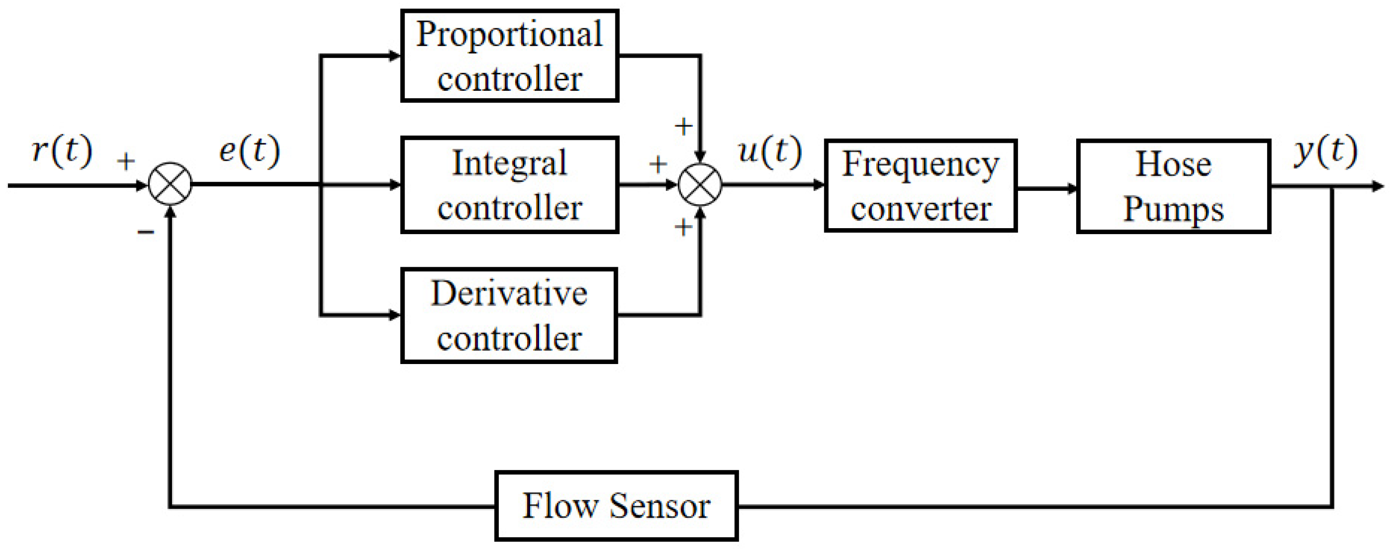
2.2.1. Conventional PID Controller Design

The conventional PID controller consists of three units: proportional, integral, and differential, which have the advantages of simple and reliable operation, high robustness, and can solve most practical applications in the industry [14]. The structure of the PID controller in this paper is shown in Figure 2.

In the controller, the set value $r\left(t\right)$ is compared with the measured value $y\left(t\right)$ to obtain the deviation $e\left(t\right)=r\left(t\right)-y\left(t\right)$. The control law gives the control quantity $u\left(t\right)$ according to the deviation $e\left(t\right)$, and the control quantity $u\left(t\right)$ is applied to the controlled object as a way to correct and regulate the response of the control system. The control quantity $u\left(t\right)$ is specifically expressed as:

$$\begin{array}{c}u\left(t\right)=K_p[e\left(t\right)+\frac{1}{T_i}{\int }_0^{t}e\left(\tau \right)d\tau +T_d\frac{de\left(t\right)}{dt}]\end{array}$$

(2)

where $K_p$ is the scaling factor.

$T_i$ is the integration time constant and $T_d$ is the differential time constant.

The above equation describes a continuous PID control algorithm, but in a real control system, the deviation value $e\left(t\right)$ needs to be obtained by sampling, so Equation (2) needs to be discretized. Assuming that the sampling period is $T$ and a total of $k$ samples are taken, the integral part of the control algorithm can be represented by Equation (3) and the differential part can be represented by Equation (4).

$$\begin{array}{c}{{\displaystyle \int }}_0^{t}e\left(t\right)dt\approx T{\displaystyle {\displaystyle \sum }_{j=0}^k}e\left(j\right)\end{array}$$

(3)

$$\begin{array}{c}\frac{de\left(t\right)}{dt}\approx \frac{e\left(kT\right)-e\left[\left(k-1\right)T\right]}{T}=\frac{e_k-e_{k-1}}{T}\end{array}$$

(4)

Bringing Equations (3) and (4) into Equation (2), the PID control algorithm expression is obtained.

$$\begin{array}{c}u\left(k\right)=K_p{e}_k+K_i{\displaystyle {\displaystyle \sum }_{j=0}^k}{e}_j+K_d\left(e_k-e_{k-1}\right)\end{array}$$

(5)

where $K_p$ is the proportionality factor, $K_i$ is the integration factor and $K_d$ is the differentiation factor; $K_i$ = $K_p\frac{T}{T_i}$, $K_d=K_p\frac{T_d}{T}$.

In this paper, the incremental PID control algorithm is used to operate on the variation of the control quantity $\Delta u\left(k\right)$, which can be obtained recursively according to Equation (5):

$$\begin{array}{c}u\left(k-1\right)=K_p{e}_{k-1}+K_i{\displaystyle {\displaystyle \sum }_{j=0}^{k-1}}{e}_j+K_d\left(e_{k-1}-e_{k-2}\right)\end{array}$$

(6)

Equation (6) is subtracted from Equation (5) to obtain:

$$\begin{array}{c}\Delta u\left(k\right)=K_p\left(e_k-e_{k-1}\right)+K_i{e}_k+K_d\left(e_k-2e_{k-1}+e_{k-2}\right)\end{array}$$

(7)

Thus, the control quantity u(k) can be expressed as:

$$\begin{array}{c}u\left(k\right)=u\left(k-1\right)+\Delta u\left(k\right)\end{array}$$

(8)

The parameter tuning of the PID controller is the core content of control system design, which determines the proportionality coefficient, integration time, and differentiation time of the PID controller according to the characteristics of the controlled process. At present, the main methods are the Cohen–Coon method, critical proportionality method, decay curve method, and other rectification methods. The common point of these methods is that the controller parameters are adjusted by test and then according to the engineering experience formula, which is simple and easy to master.

The Cohen–Coon method is used to initially rectify the three parameters $K_p$, $T_i$, and $T_d$. The Cohen–Coon method is mainly used to obtain the optimal PID parameter rectification value by configuring the dominant pole of the system so that the transition curve of the object decays at a decay rate of 4:1 [15]. The rectification equation is shown in Equation (9).

$$\{\begin{array}{l}{K}_p=\frac{T}{K\tau }\left(\frac{4}{3}+\frac{\tau }{4T}\right)\\ T_i=\tau \left(\frac{32+\frac{6\tau }{T}}{13+\frac{8\tau }{T}}\right)\\ T_d=\tau \left(\frac{4}{11+\frac{2\tau }{T}}\right)\end{array}$$

(9)

The mathematical model of the control object is shown in Equation (1), and the corresponding parameters are brought into Equation (1) to obtain $K_p$ = 0.69, $K_i$ = 0.05, and $K_d$ = 1.78.

Although PID control can solve most engineering problems, it also has shortcomings, for example, the control parameters of conventional PID cannot follow changes dynamically, so it is difficult to obtain better control results when it is applied to complex systems [16].

2.2.2. BP Neural Network-Based PID Controller Design

The BP neural network-based PID controller can dynamically adjust the parameters of the PID through the autonomous learning capability of the neural network, thus replacing the human empirical values and making the parameters achieve the best control according to the changes in the environment [17,18].

According to the characteristics of cooperation and constraints of three parameters $K_p$, $K_i$, and $K_d$ of PID control, the mapping ability of the BP neural network to nonlinear functions is used to obtain the optimal solution for the nonlinear combination of the three parameters. The structure of the BP neural network-based PID controller is shown in Figure 3.

The structure is divided into two parts. Bulleted lists look like this:

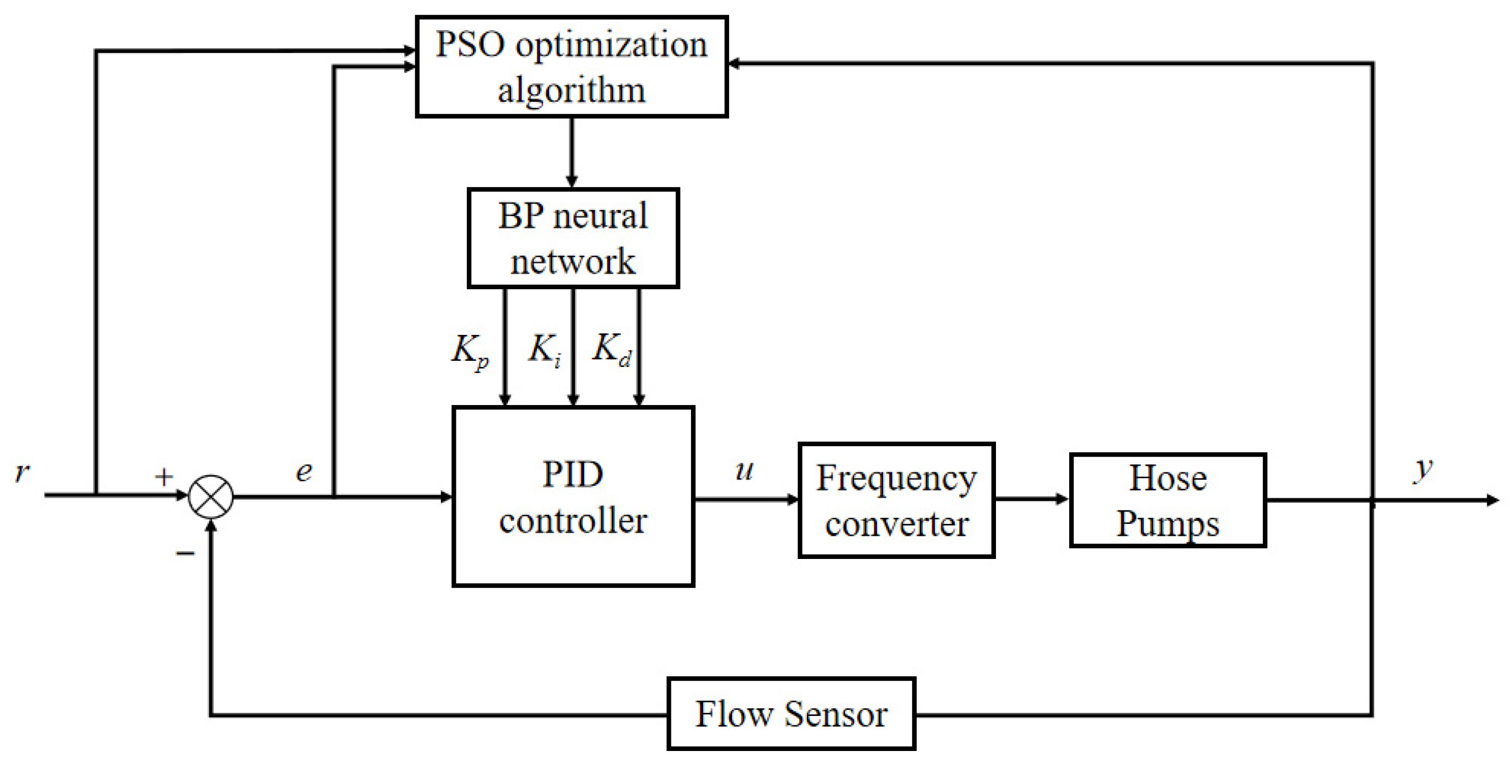
• Conventional PID controller generates control quantities through $K_p$, $K_i$, $K_d$ output from BP neural network to realize feedback control of controlled objects.
• The BP neural network provides optimal parameters for the PID controller based on the system operating state and the learning algorithm.

The network structure is shown in Figure 4.

The input of neurons in the input layer of the neural network is the output:

$$\begin{array}{c}{O}_j{}^{\left(1\right)}=x\left(j\right) \left(j=1,2,\dots ,M\right)\end{array}$$

(10)

where $M$ is the number of input layer variables of the neural network, which can be adjusted according to the complexity of the controlled object, and the input layer variables in this paper are expected value, actual value, error, and network threshold.

The input and output of the implicit layer neurons are:

$$\begin{array}{c}ne{t}_i{}^{\left(2\right)}={{\displaystyle \sum }}_{j=0}^M{w}_{ij}{}^{\left(2\right)}{O}_j{}^{\left(1\right)}\end{array}$$

(11)

$$\begin{array}{c}{O}_i^{\left(2\right)}\left(k\right)=f\left(ne{t}_i^{\left(2\right)}\left(k\right)\right) \left(i=1,2,\dots ,Q\right)\end{array}$$

(12)

where $Q$ is the number of neurons in the hidden layer, which is set to 5 in order to simplify the complexity of the system and accelerate the learning speed. $w_{ij}{}^{\left(2\right)}$ denotes the weight between the $i$th neuron in the hidden layer and the $j$th neuron in the input layer, and the continuous function can be approximated with arbitrary accuracy in the neural network using the Sigmoid function, so the transformation function of the hidden layer is chosen as the positive and negative symmetric Sigmoid function, as in Equation (13).

$$\begin{array}{c}f\left(x\right)=\frac{e^x-e^{-x}}{e^x+e^{-x}}\end{array}$$

(13)

The output layer neuron inputs and outputs are:

$$\begin{array}{c}ne{t}_l{}^{\left(3\right)}\left(k\right)={{\displaystyle \sum }}_{i=0}^Q{w}_{li}{}^{\left(3\right)}{O}_i{}^{\left(2\right)}\left(k\right)\end{array}$$

(14)

$$\begin{array}{c}{O}_l^{\left(3\right)}\left(k\right)=g\left(ne{t}_l^{\left(3\right)}\left(k\right)\right) \left(l=1,2,3\right)\end{array}$$

(15)

where $w_{li}{}^{\left(3\right)}$ denotes the weight between the $l$th neuron of the output layer and the $i$th neuron of the input layer, and the three outputs of the output layer correspond to the three adjustable parameters $K_p$, $K_i$, and $K_d$ of the PID controller, respectively. Since $K_p$, $K_i$, and $K_d$ cannot be negative, the transformation function of the output layer neurons is taken as a non-negative Sigmoid function, as in Equation (16).

$$\begin{array}{c}g\left(x\right)=\frac{e^x}{e^x+e^{-x}}\end{array}$$

(16)

To ensure the real-time performance of the system, the online learning method is used, and the quadratic of the error is used as the performance indicator, so the performance indicator function is chosen as:

$$\begin{array}{c}E\left(k\right)=\frac{1}{2}{\left[r\left(k\right)-y\left(k\right)\right]}^2\end{array}$$

(17)

The gradient descent method is used to adjust the weights of each layer of the BP neural network in the direction of the negative gradient of $E$ [19]. To improve the convergence speed, the inertia term with α as the inertia factor is added.

$$\begin{array}{c}\Delta w_{li}^{\left(3\right)}\left(k\right)=-\eta \frac{\partial E\left(k\right)}{\partial w_{li}^{\left(3\right)}}+\alpha \Delta w_{li}^{\left(3\right)}\left(k-1\right)\end{array}$$

(18)

where $\eta$ is the learning rate and $\alpha$ is the inertia factor, according to the chain rule we get:

$$\begin{array}{c}\frac{\partial E\left(k\right)}{\partial w_{li}^{\left(3\right)}}=\frac{\partial E\left(k\right)}{\partial y\left(k\right)}\times \frac{\partial y\left(k\right)}{\partial \Delta u\left(k\right)}\times \frac{\partial \Delta u\left(k\right)}{\partial O_l^{\left(3\right)}\left(k\right)}\times \frac{\partial O_l^{\left(3\right)}\left(k\right)}{\partial ne{t}_l^{\left(3\right)}\left(k\right)}\times \frac{\partial ne{t}_l^{\left(3\right)}\left(k\right)}{\partial w_{li}^{\left(3\right)}\left(k\right)}\end{array}$$

(19)

After simplification and approximation, the final amount of regulation between the weight of the $l$th neuron in the output layer and the $i$th neuron in the hidden layer after learning is obtained as:

$$\begin{array}{c}\frac{\partial E\left(k\right)}{\partial w_{li}^{\left(3\right)}}=\frac{\partial E\left(k\right)}{\partial y\left(k\right)}\ast \frac{\partial y\left(k\right)}{\partial \Delta u\left(k\right)}\ast \frac{\partial \Delta u\left(k\right)}{\partial O_l^{\left(3\right)}\left(k\right)}\ast \frac{\partial O_l^{\left(3\right)}\left(k\right)}{\partial ne{t}_l^{\left(3\right)}\left(k\right)}\ast \frac{\partial ne{t}_l^{\left(3\right)}\left(k\right)}{\partial w_{li}^{\left(3\right)}\left(k\right)}\end{array}$$

(20)

$$\begin{array}{c}\Delta w_{li}^{\left(3\right)}\left(k\right)=\alpha \Delta w_{li}^{\left(3\right)}\left(k-1\right)+\eta {\delta }_l^{\left(3\right)}{O}_i^{\left(2\right)}\left(k\right)\end{array}$$

(21)

$$\begin{array}{c}{\delta }_l^{\left(3\right)}=e\left(k\right)sgn\left(\frac{\partial y\left(k\right)}{\partial \Delta u\left(k\right)}\right)\frac{\partial \Delta u\left(k\right)}{\partial O_l^{\left(3\right)}\left(k\right)}{g}^{\prime }\left(ne{t}_l^{\left(3\right)}\left(k\right)\right) \left(l=1,2,3\right)\end{array}$$

(22)

Similarly, the amount of weight regulation between the $i$th neuron in the hidden layer and the $j$th neuron in the input layer can be obtained as:

$$\begin{array}{c}\Delta w_{ij}^{\left(2\right)}\left(k\right)=\alpha \Delta w_{ij}^{\left(2\right)}\left(k-1\right)+\eta {\delta }_i^{\left(2\right)}{O}_j^{\left(1\right)}\left(k\right)\end{array}$$

(23)

$$\begin{array}{c}{\delta }_i^{\left(2\right)}=f^{\prime }\left(ne{t}_i^{\left(2\right)}\left(k\right)\right){\displaystyle {\displaystyle \sum }_{l=1}^3}{\delta }_l^{\left(3\right)}{w}_{li}^{\left(3\right)}\left(k\right) \left(i=1,2,\dots Q\right)\end{array}$$

(24)

In summary, Equations (20) and (22) are the calculation equations for the regulation amount of the weight coefficients of each layer of the network. The BP neural network algorithm flow is shown in Figure 5.

The inclusion of the BP neural network algorithm in the PID controller enables the dynamic regulation of the PID parameters, but due to the gradient descent method, the BP neural network converges more slowly and is prone to local minima when trained in places where the error curve is flat [20]. Therefore, this paper makes use of the global optimum and fast convergence of the Particle Swarm algorithm to improve the BP neural network and optimize the initial weights of the BP neural network, to overcome the defects that the neural network is prone to fall into local minima and slow convergence speed.

2.2.3. BP Neural Network PID Controller Design Based on PSO Optimization

The Particle Swarm Optimization (PSO) algorithm, first proposed by Eberhart and Kennedy in 1995, is an intelligent algorithm designed by simulating the predatory behavior of a flock of birds. Its basic core is to use the sharing of information by individuals in the group to continuously update their position and velocity information, thus making the motion of the whole group produce an evolutionary process from disorder to order in the problem-solving space, and finally obtaining the optimal solution of the problem [21,22].

The structure of the BP neural network PID controller based on PSO optimization is shown in Figure 6.

The PSO algorithm is described in detail as follows:

In the PSO algorithm, each particle possesses two attributes: velocity $V$ and position $X$. $V$ represents the speed of particle movement, and $X$ determines the direction of particle search. Assume that in a D-dimensional search space, a population $X=\left(X_1,X_2,\dots ,X_n\right)$ is composed of $n$ particles, and the position and velocity of the ith particle are denoted as follows:

$$\begin{array}{c}{X}_i=\left(x_{i1},x_{i2},\dots ,x_{iD}\right) \left(i=1,2,\dots ,n\right)\end{array}$$

(25)

$$\begin{array}{c}{V}_i=\left(v_{i1},v_{i2},\dots ,v_{iD}\right) \left(i=1,2,\dots ,n\right)\end{array}$$

(26)

where $X_i$ represents not only the particle position, but also a potential solution to the problem, i.e., the initial weights of a set of BP neural networks. The fitness value corresponding to each particle position can be calculated by substituting $X_i$ into the fitness function.

The current individual optimal solution $P_{best}$ of the particle, and the current global optimal solution $g_{best}$ of the whole particle population will be used as the basis for updating $V$ and $X$ in the optimization search process.

$$\begin{array}{c}{P}_{best}=\left(P_{i1},P_{i2},\dots ,P_{iD}\right) \left(i=1,2,\dots ,n\right)\end{array}$$

(27)

$$\begin{array}{c}{g}_{best}=\left(g_1,g_2,\dots ,g_D\right) \end{array}$$

(28)

$V$ and $X$ of the particle are updated by Equations (28) and (29), respectively.

$$\begin{array}{c}{v}_{id}^{k+1}=w_k{v}_{id}^k+c_1{r}_1\left(P_{id}^k-x_{id}^k\right)+c_2{r}_2\left(g_d^k-x_{id}^k\right)\end{array}$$

(29)

$$\begin{array}{c}{x}_{id}^{k+1}=x_{id}^k+v_{id}^{k+1}\end{array}$$

(30)

where $d=1,2,\dots ,D$; $i=1,2,\dots ,n$; $k$ is the number of current iterations; $w_k$ is the inertia weight; $c_1$, $c_2$ are learning factors, generally take $c_1=c_2=$2; $r_1$, $r_2$ are generally taken as random numbers in the range of [0, 1].

The inertia weight $w_k$ decreases as the number of iterations increases.

$$\begin{array}{c}{w}_k=w_s-\left(k-1\right)\frac{\left(w_s-w_e\right)}{T_{max}}\end{array}$$

(31)

where $w_s$ and $w_e$ are the upper and lower bounds of inertia weights in the range of [0.4, 0.9], respectively, and $T_{max}$ is the maximum number of iterations.

In this paper, Equation (17) is used as the fitness function of the PSO algorithm, and since the optimization object is the weight of the BP neural network and the neural network structure is 4 − 5 − 3, the dimension D is set to 4 × 5 + 3 × 5 = 35, the maximum number of iterations is set to 50, the particle swarm size is taken as 20, and the initial weights of 20 groups of BP neural network are generated randomly. To prevent the particles from searching blindly, the position $X$ and velocity $V$ are limited to a certain range. The PSO optimization algorithm flow is shown in Figure 7.

3. Results

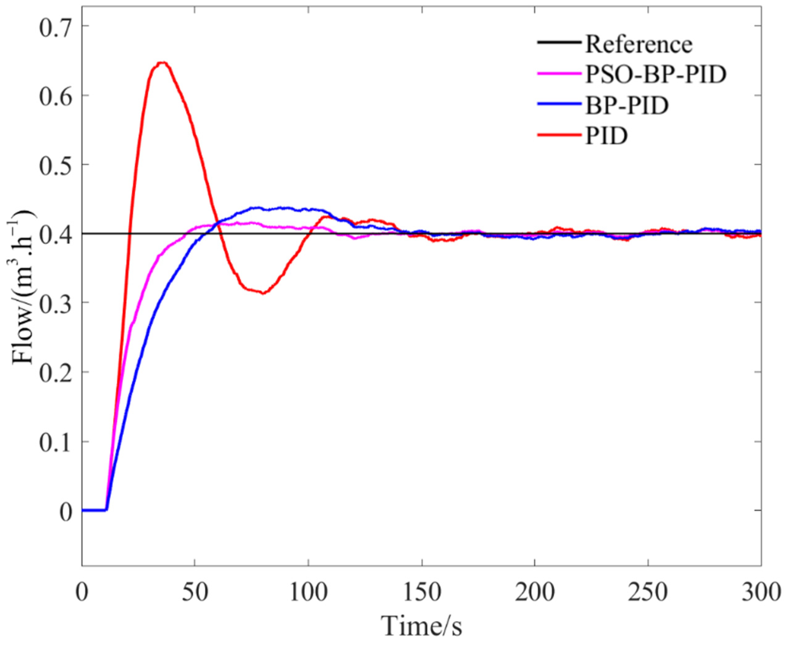
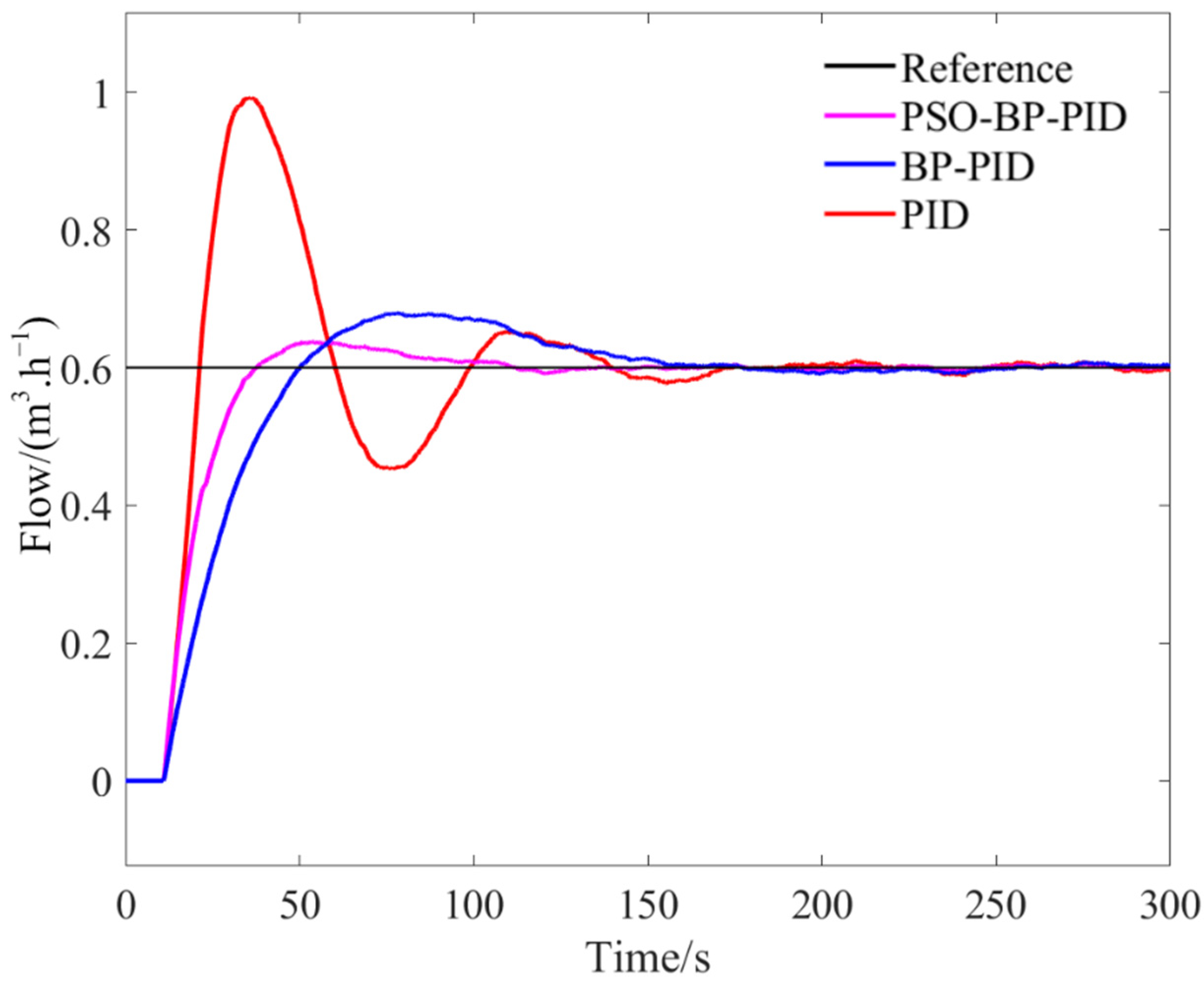
3.1. Analysis of Simulation Results

Matlab software was used for simulation, and three different control methods were used in the simulation experiments, namely: conventional PID control, BP neural network-based PID control (BP-PID control), and PSO optimization-based BP neural network PID control (PSO-BP-PID control). The unit step was used as input signal, respectively, and the simulation time was 100 s. The simulation results are as follows:

Figure 8 shows the iterative process of the PSO algorithm under unit step response, and the optimal individual adaptation value was obtained after 50 iterations. Figure 9 shows the comparison of the control effects of the three controllers under the unit step response.

The dynamic performance index was used to evaluate the control effect of the controller, where the rise time indicates the time when the system is excited by the step signal and reaches the steady-state value for the first time; the peak time indicates the time when the system is excited by the step response and reaches the peak; the regulation time indicates the time required for the system to reach stability, i.e., to enter the error tolerance range; the maximum overshoot reflects the controller control process stability. The dynamic performance of the three controllers is shown in

Table 1. Dynamic performance of the three controllers.

Controller Type	Rise Time (s)	Peak Time (s)	Regulation Time (s)	Maximum Overshoot
PID	12.41	13.62	25.07	58.53%
BP-PID	14.69	16.73	19.68	20.74%
PSO-BP-PID	11.97	12.31	11.77	3.19%

.

From Figure 9 and Table 1, it can be seen that the conventional PID controller produced larger oscillation and overshoot, with 58.23% overshoot and longer regulation time although the rise time was shorter; compared with the conventional PID controller, the BP-PID controller had a longer rise time and peak time but the overall response was relatively stable and the overshoot was reduced to 20.74%; the PSO-BP-PID controller compared with the other two controllers, the dynamic performance has been significantly improved, not only were the rise time and regulation time shortened to 11.97 s and 11.77 s, respectively, but also the overshoot amount was 3.19%, and the response was more rapid and smooth.

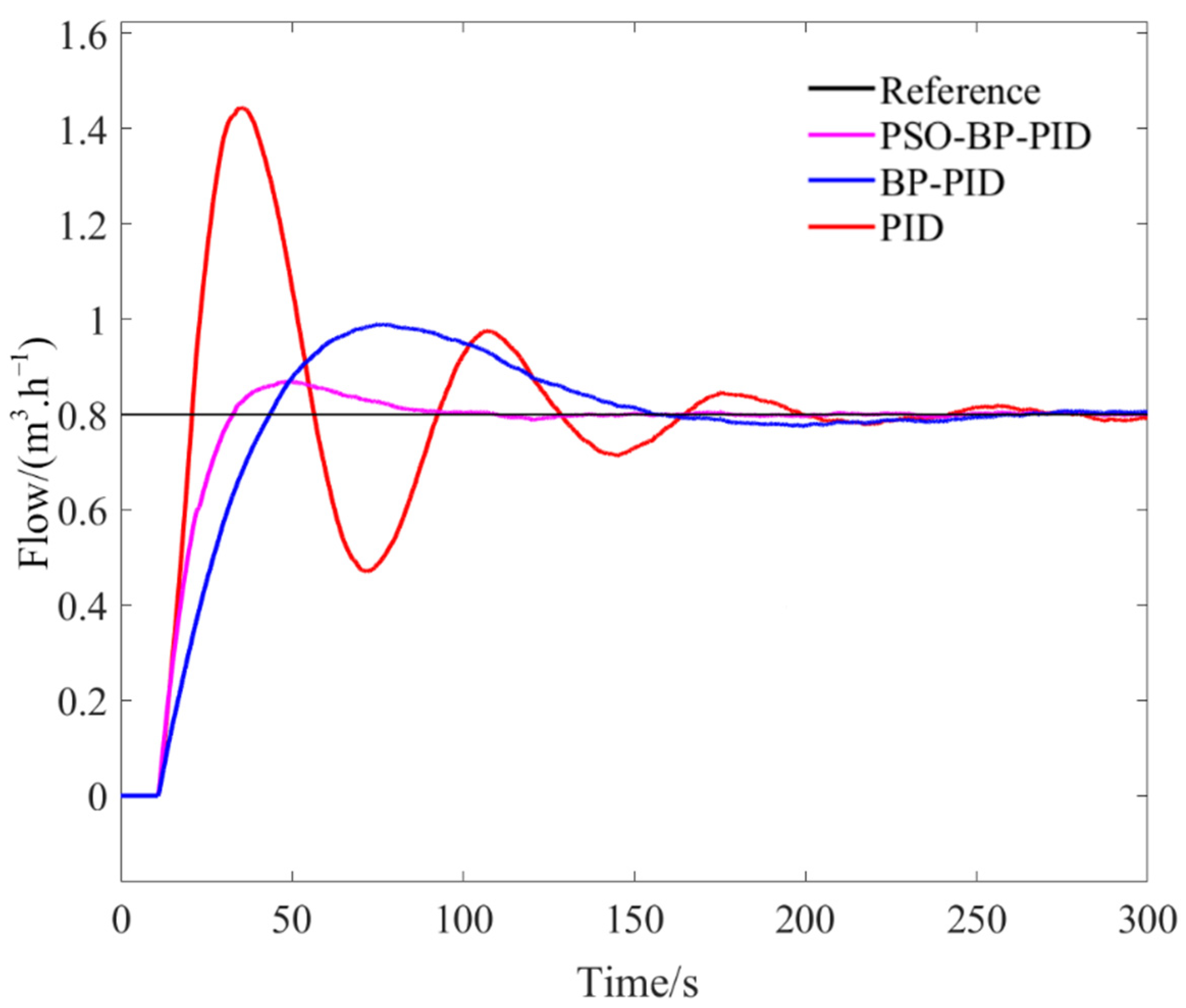
3.2. Precision Fertilizer Control System Flow Regulation Test

3.2.1. Testing Device and System Design

To verify the practical performance of the PSO-BP-PID algorithm, a corresponding flow rate regulation test platform was built for this paper. Using the STM32F103ZET6 microcontroller as the control element, the signal from the flow sensor received at the I/O port was calculated inside the microcontroller and converted into a variable voltage signal to adjust the output frequency of the inverter and finally changed the fertilizer flow rate at the outlet of the mixing tank. The maximum conveying flow of the hose pump is 1 m³/h, rated power is 1.5 kW, and rated voltage is 380 V. The frequency converter is rated at 2.2 kW, with an output frequency between 0 and 400 Hz and a rated voltage of 380 V. The flow sensor was selected from the stainless-steel electromagnetic flowmeter of Meacon China, model LDG-MIK, with an accuracy of 0.5%. The volume of liquid in the mixing tank was kept at 50 L during operation. The flow rate regulation test platform is shown in Figure 10.

The USB-1252A data collector from Smacq was used to collect the data needed in the test. The collector has an advanced measurement and control system with 16 analog input channels, 12-bit vertical resolution, and up to 500 kSa/s analog acquisition capability. The schematic diagram of the data acquisition and control system is shown in Figure 11.

3.2.2. Analysis of Test Results

The fertilized crop in this paper is cotton, and since the fertilizer flow rate is determined by the fertilizer demand of the crop, the fertilizer demand of cotton is different in different growing periods. The flow rate of the hose pump at the outlet of the mixing tank was set to 0.4 m³/h, 0.6 m³/h, and 0.8 m³/h in turn, and the performance of the three controllers was tested. The test results are shown in Figure 12, Figure 13 and Figure 14, and the performance indexes of the three controllers are shown in

Table 2. Comparison of the dynamic performance of three controllers at fertilizer application flow rate of 0.4 m³/h.

Controller Type	Rise Time (s)	Peak Time (s)	Regulation Time (s)	Maximum Overshoot	Root Mean Square Error
PID	21.33	34.97	90.51	61.95%	0.058
BP-PID	54.88	87.47	43.10	9.55%	0.015
PSO-BP-PID	46.27	68.37	31.36	4.08%	0.004

,

Table 3. Comparison of the dynamic performance of three controllers at fertilizer application flow rate of 0.6 m³/h.

Controller Type	Rise Time (s)	Peak Time (s)	Regulation Time (s)	Maximum Overshoot	Root Mean Square Error
PID	21.22	36.05	115.86	65.27%	0.084
BP-PID	50.13	77.97	112.52	13.15%	0.028
PSO-BP-PID	37.53	53.36	30.85	6.23%	0.014

and

Table 4. Comparison of the dynamic performance of three controllers at fertilizer application flow rate of 0.8 m³/h.

Controller Type	Rise Time (s)	Peak Time (s)	Regulation Time (s)	Maximum Overshoot	Root Mean Square Error
PID	20.80	34.97	155.83	80%	0.125
BP-PID	43.50	74.94	131.46	23.75%	0.070
PSO-BP-PID	32.76	48.64	61.30	8.75%	0.027

.

The results in Table 2, Table 3 and Table 4 showed that the performance of the three controllers also changed with the increase in fertilizer flow rate. The conventional PID controller had the fastest rise time at all three fertilizer flow rates, but the overshoot was large and the flow rate had large fluctuations and could not reach the desired value quickly; the BP-PID controller had significantly less overshoot compared with the conventional PID controller, but the response speed was slower; the PSO-BP-PID controller had the minimum overshoot and root-mean-square error at all three fertilizer flow rates, and could balance the response speed and stability of the control process at higher flow rates with good robustness to meet the control requirements in practical applications.

In recent years, the need to improve water use efficiency in irrigated agriculture has attracted a great deal of attention from researchers. The PSO-BP-PID controller developed in this paper uses a closed-loop intelligent irrigation feedback control strategy to greatly improve the efficiency of irrigation water use in the field and provide ideas for future water sustainability.

4. Conclusions

In this paper, the precision fertilizer control system was studied, its mathematical model was fitted, and the transfer function of the system was obtained. Based on the BP neural network PID adaptive control, a PSO optimization algorithm was added to optimize the initial weights of the neural network, and a BP neural network PID controller based on PSO optimization was designed, and the dynamic performance of the three controllers, PID, BP-PID, and PSO-BP-PID, were compared and analyzed.

The test results showed that the PSO-BP-PID controller was significantly better than the other two controllers in terms of control accuracy and adjustment time. At the fertilizer application flow rate of 0.4 m³/h, 0.6 m³/h, and 0.8 m³/h, respectively, the set value was reached quickly with an average maximum overshoot of 6.35% and an average adjustment time of 41.17 s. Among them, the shortest adjustment time was 30.85 s when the fertilizer application flow rate was at 0.6 m³/h. This indicates that the controller has the best control of irrigation fertilization at this flow rate.

The BP neural network PID control algorithm based on PSO optimization can adjust the PID parameters online according to changes of the environment, which improves the decision making of the controller. The algorithm reasonably determines the initial weights of the BP neural network; it solves the problems that the BP neural network easily falls into local minima and converges slowly; and not only approximates the control target faster, but also has a shorter response time; thus providing a feasible method for the control of nonlinear time-lag systems.

References

1. Silber, A.; Xu, G.; Levkovitch, I.; Soriano, S.; Bilu, A.; Wallach, R. High fertigation frequency: The effects on uptake of nutrients, water and plant growth. Plant Soil 2003, 253, 467–477. [Google Scholar] [CrossRef]
2. Wang, H.; Li, J.; Cheng, M.; Zhang, F.; Wang, X.; Fan, J.; Wu, L.; Fang, D.; Zou, H.; Xiang, Y. Optimal drip fertigation management improves yield, quality, water and nitrogen use efficiency of greenhouse cucumber. Sci. Hortic. 2019, 243, 357–366. [Google Scholar] [CrossRef]
3. Xiuyun, X.; Xufeng, X.; Zelong, Z.; Bin, Z.; Shuran, S.; Zhen, L.; Tiansheng, H.; Huixian, H. Variable Rate Liquid Fertilizer Applicator for Deep-fertilization in Precision Farming Based on ZigBee Technology. IFAC-PapersOnLine 2019, 52, 43–50. [Google Scholar] [CrossRef]
4. Ying-Zi, Z.; Hai-Tao, C.; Shou-Yin, H.; Wen-Yi, J.; Bin-Lin, O.; Guo-Qiang, D.; Ji-Cheng, Z. Design and Experiment of Slave Computer Control System for Applying Variable-rate Liquid Fertilizer. J. Northeast Agric. Univ. 2015, 22, 73–79. [Google Scholar] [CrossRef]
5. Zou, Z.; Yu, M.; Wang, Z.; Liu, X.; Guo, Y.; Zhang, F.; Guo, N. Nonlinear Model Algorithmic Control of a pH Neutralization Process. Chin. J. Chem. Eng. 2013, 21, 395–400. [Google Scholar] [CrossRef]
6. Lai, Z.; Wu, P.; Wu, D. Application of fuzzy adaptive control to a MIMO nonlinear time-delay pump-valve system. ISA Trans. 2015, 57, 254–261. [Google Scholar] [CrossRef]
7. Dong, Y.; Fu, Z.; Peng, Y.; Zheng, Y.; Yan, H.; Li, X. Precision fertilization method of field crops based on the Wavelet-BP neural network in China. J. Clean. Prod. 2020, 246, 118735. [Google Scholar] [CrossRef]
8. Feng, G.; Lei, S.; Gu, X.; Guo, Y.; Wang, J. Predictive control model for variable air volume terminal valve opening based on backpropagation neural network. Build. Environ. 2021, 188, 107485. [Google Scholar] [CrossRef]
9. Jesus, I.S.; Barbosa, R.S. Smith-fuzzy fractional control of systems with time delay. AEU Int. J. Electron. Commun. 2017, 78, 54–63. [Google Scholar] [CrossRef]
10. Bai, J.; Tian, M.; Li, J. Control System of Liquid Fertilizer Variable-Rate Fertilization Based on Beetle Antennae Search Algorithm. Processes 2022, 10, 357. [Google Scholar] [CrossRef]
11. Fu, Q.; Wang, Z.; Jiang, Q. Delineating soil nutrient management zones based on fuzzy clustering optimized by PSO. Math. Comput. Model. 2010, 51, 1299–1305. [Google Scholar] [CrossRef]
12. Navarro, J.L.; Díez, J.L.; Valera, A.; Valles, M. Remote Fuzzy Control of a DC Motor. IFAC Proc. Vol. 2008, 41, 13652–13658. [Google Scholar] [CrossRef]
13. Estofanero, L.; Edwin, R.; Claudio, G. Predictive Controller Applied to a pH Neutralization Process. IFAC-PapersOnLine 2019, 52, 202–206. [Google Scholar] [CrossRef]
14. Zhao, C.; Guo, L. Towards a theoretical foundation of PID control for uncertain nonlinear systems. Automatica 2022, 142, 110360. [Google Scholar] [CrossRef]
15. Joseph, S.B.; Dada, E.G.; Abidemi, A.; Oyewola, D.O.; Khammas, B.M. Metaheuristic algorithms for PID controller parameters tuning: Review, approaches and open problems. Heliyon 2022, 8, e09399. [Google Scholar] [CrossRef]
16. Chang, W.-D.; Shih, S.-P. PID controller design of nonlinear systems using an improved particle swarm optimization approach. Commun. Nonlinear Sci. Numer. Simul. 2010, 15, 3632–3639. [Google Scholar] [CrossRef]
17. Tang, G.; Lei, J.; Du, H.; Yao, B.; Zhu, W.; Hu, X. Proportional-integral-derivative controller optimization by particle swarm optimization and back propagation neural network for a parallel stabilized platform in marine operations. J. Ocean Eng. Sci. 2022. [Google Scholar] [CrossRef]
18. Li, H.; Zhen-Yu, Z. The application of immune genetic algorithm in main steam temperature of PID control of BP network. Phys. Procedia 2012, 24, 80–86. [Google Scholar] [CrossRef]
19. Huang, G.; Yuan, X.; Shi, K.; Wu, X. A BP-PID controller-based multi-model control system for lateral stability of distributed drive electric vehicle. J. Frankl. Inst. 2019, 356, 7290–7311. [Google Scholar] [CrossRef]
20. Huang, J.; He, L. Application of Improved PSO—BP Neural Network in Customer Churn Warning. Procedia Comput. Sci. 2018, 131, 1238–1246. [Google Scholar] [CrossRef]
21. Ren, C.; An, N.; Wang, J.; Li, L.; Hu, B.; Shang, D. Optimal parameters selection for BP neural network based on particle swarm optimization: A case study of wind speed forecasting. Knowl. Based Syst. 2014, 56, 226–239. [Google Scholar] [CrossRef]
22. Zhang, J.-R.; Zhang, J.; Lok, T.-M.; Lyu, M.R. A hybrid particle swarm optimization–back-propagation algorithm for feedforward neural network training. Appl. Math. Comput. 2007, 185, 1026–1037. [Google Scholar] [CrossRef]
Figure 1. Structure diagram of precision fertilization control system: 1. Reservoir; 2. Fertilizer tank; 3. Filter; 4. One-way valve; 5. Pressure regulator; 6. Flow sensor; 7. Pressure gauge; 8. Mixing tank; 9. Agitator pump; 10. Y-filter; 11. Hose pump; 12. Pressure holding valve; 13. Master valve; 14. Branch valve; 15. Drip irrigation belt; 16–19. Solenoid valve.
Agriculture 12 01395 g001
Figure 2. Conventional PID controller structure.
Agriculture 12 01395 g002
Figure 3. Structure of the BP neural network-based PID controller.
Agriculture 12 01395 g003
Figure 4. BP neural network structure.
Agriculture 12 01395 g004
Figure 5. BP neural network algorithm process.
Agriculture 12 01395 g005
Figure 6. Structure of BP neural network PID controller based on PSO optimization.
Agriculture 12 01395 g006
Figure 7. PSO optimization algorithm process.
Agriculture 12 01395 g007
Figure 8. Iterative process of PSO algorithm under unit step response.
Agriculture 12 01395 g008
Figure 9. Comparison of the control effect of three controllers under unit step response.
Agriculture 12 01395 g009
Figure 10. Flow regulation test platform.
Agriculture 12 01395 g010
Figure 11. Schematic diagram of data acquisition and control system.
Agriculture 12 01395 g011
Figure 12. Regulation curves of three controllers at fertilizer application flow rate of 0.4 m3/h.
Agriculture 12 01395 g012
Figure 13. Regulation curves of the three controllers at a fertilizer application flow rate of 0.6 m3/h.
Agriculture 12 01395 g013
Figure 14. Regulation curves of the three controllers at a fertilizer application flow rate of 0.8 m3/h.
Agriculture 12 01395 g014