
Characterizing Agricultural Diversity with Policy-Relevant Farm Typologies in Mexico


Department of Geography, The University of Alabama, Tuscaloosa, AL 35487, USA
Agriculture 2022, 12(9), 1315; https://doi.org/10.3390/agriculture12091315
Submission received: 27 July 2022
/
Revised: 19 August 2022
/
Accepted: 24 August 2022
/
Published: 26 August 2022
(This article belongs to the Section Agricultural Economics, Policies and Rural Management)
Abstract
:The effective targeting of agricultural policy interventions across heterogenous agricultural landscapes requires an integrated understanding of farm diversity. One pathway to this understanding is through farm typologies—classification systems that synthesize farm complexity into a limited number of ‘types’. Farm typologies are typically constructed at local or regional levels and seldom demonstrate policy relevance through example. This study has two objectives: (1) to construct a policy-relevant farm typology that characterizes agricultural diversity in Mexico, and (2) to demonstrate, through case study example, how the typology could be used to target policy interventions. Hierarchical agglomerative cluster (HAC) analysis is used to group municipalities (n = 2455) based on farm characteristics (n = 10) and cropping patterns (n = 10). Two clustering solutions were chosen based on statistical goodness-of-fit measures and topical relevance. The first set of clusters (Typology A) grouped municipalities into one of three types: (A1) southern lowland farms, (A2) northern midland farms, and (A3) southern-central highland farms. The second (Typology B) grouped municipalities into 12 sub-types illustrating lower-order distinctions. Each typology was described, validated, and mapped at the national level. The typologies were then used to illustrate the targeting soil erosion interventions across Mexico. Here, multiple correspondence analysis (MCA) was used to examine relationships between the typologies and two priority targeting criteria. Farms of the southern lowland region (Type A1) and two of its subtypes (B1 and B12) were identified as priority areas for interventions. In sum, this study: (1) creates a series of new, typology-based conceptualizations of regional agricultural diversity in Mexico, and (2) demonstrates how such typologies can serve as actionable tools for agricultural policy.
1. Introduction
Characterizing the diversity of farm systems is important for agricultural policymaking and for understanding the multifunctional nature of agricultural systems. Too often, farm diversity is lost under ‘one-size-fits-all’ approaches to policy based on singular objectives such as production stabilization or income support [1,2,3]. This contrasts with the conceptual goals of many agricultural policies, which have broadened in recent decades to address not only food and fiber production, but also environmental, rural development, and energy concerns [4,5,6,7]. Agricultural research also has broadened in recent decades to incorporate systems-based approaches for addressing sustainability, ecosystem services, climate resilience, rural poverty, and other transdisciplinary issues. In sum, as agricultural research and policy concerns have broadened, the need to synthesize farm diversity into informative and useful frameworks has grown.
Farm typology research specializes in synthesizing farm complexity and organizing it into a limited number of distinct classes or ‘types’ [8]. Typically, these types are constructed by grouping farms by structural characteristics such as production input (land, labor, capital) or output factors (income, productivity measures). Other typologies are constructed around farm functional or social characteristics such as farmer behavior or decision-making processes in response to disturbances [9,10]. Typology research is exploratory in that unsupervised learning methods are often used to reveal underlying structural relationships between farm system attributes. Ultimately, these relationships are used to define the boundaries between farm systems as distinct ‘types’ [11,12].
Three trenchant critiques of farm typology research center on: (1) the lack of policy relevance [13], the sometimes-arbitrary logic behind typology construction [14], and the overreliance on farm structural variables as defining characteristics [10]. Collectively, studies are beginning to address these critiques by emphasizing participatory approaches to typology construction and validation, and by formally recognizing these limitations. Studies increasingly refer to the policy-relevance of typologies, often in the context of ‘targeting’ policy interventions, though few studies actually demonstrate how typologies can be used as such [1,13,15,16]. Therefore, many opportunities remain for demonstrating how targeting by type, instead of by singular attributes, allows for better management of farm complexity and the potential synergies or spillover effects that result from policy interventions.
Farm typologies typically are constructed at the community, state, or regional scale. This is in part due to the scale-dependency of the participatory approaches often used in typology construction and validation [17,18,19]. Further, at the national level, multidimensional data on farm-level characteristics are often unavailable, especially in lower-income countries, which often lack institutional support [20,21]. National agricultural censuses often serve as valuable data sources but are sometimes carried out inconsistently due to high costs or logistical challenges [22]. Despite these limitations, national-level census data provide key insights into agricultural diversity. Understanding this diversity over large spatial scales is key for downscaling national policies equitably and in accordance with stated policy objectives [23,24,25].
Farm classification maps have long been used for this purpose, even though traditional classification maps tend to focus first on singular dimensions related to productivity or economic factors, and only incrementally add other attributes of interest [26,27]. In the United States, some traditional farm classification or production regions maps have been combined with typology studies to produce Farm Resource Regions maps [28]. These maps have been used by the US Department of Agriculture to examine farm diversity nationally and, in part, to determine program funding priorities [29,30]. Collectively, typology-based mapping approaches serve to update previous conceptualizations of farm diversity, providing useful frameworks for addressing an increasingly broad set of agricultural policy objectives [31,32,33,34].
In Mexico, farm regions maps based on typology-like integration of farm structural and functional characteristics are seldom available at the national level. Existing maps focus primarily on baseline physiographic, climatic, and edaphic factors [35,36]. Others illustrate the distribution of important crops, often stratified by irrigated and rainfed cultivation strategies [37,38]. Multidimensional data on farm characteristics are available through the website of Mexico’s National Institute of Statistics and Geography (INEGI) (https://www.inegi.org.mx/default.html, accessed on 10 September 2021); many of these data derive from Mexico’s most recent national agricultural census (2007), a monumental effort conducted after a long delay following the previous census in 1991 [39]. Other data derive from the Agri-food and Fisheries Service database of the Secretary of Agriculture and Rural Development, which includes the official yearly totals of crop production across the country [37]. Together, these sources represent the most complete accounting of agricultural activities across Mexico—data that are essential for synthesizing farm complexity into a coherent and policy-relevant form.
In sum, the above review identifies several research gaps or needs. First, a strong need exists for research that synthesizes farm system complexity into actionable and policy-relevant farm types or regions. Such synthesis is key for agricultural policymaking. Second, better understanding of farm diversity and complexity at larger scales (e.g., national levels) is needed to match the scale of agricultural policies during the early stages of work among scaling organizations. Third, while studies increasingly acknowledge the usefulness of typology research for agricultural policymaking, few have demonstrated how such typologies can serve as actionable tools for targeting policy interventions. This gap in the literature is especially evident in Mexico, where existing farm regions maps tend to focus on singular biophysical or cropping characteristics, instead of on the integration of diverse farm structural and functional characteristics.
To address these gaps, this paper has two main objectives:
- Construct, classify, and validate a national-level typology of farm characteristics and cropping patterns that better reflects the diversity and complexity of agricultural systems in Mexico.
- Demonstrate how the typology could serve as a tool for targeting agricultural policy interventions.
To these ends, this study uses data from the above sources to construct a national-level farm typology of 2455 municipalities in Mexico. Hierarchical agglomerative cluster (HAC) analysis is used to group municipalities into two typologies based on 10 farm structural and functional characteristics and the production attributes of 10 important crop species. The first typology (A) is comprised of three distinct classes of farms and is designed as a broad, general farm classification. The second typology (B) is a sub-grouping of the first that is comprised of 12 additional classes that highlight lower-order distinctions. Each typology is validated statistically, mapped, and analyzed in relation to existing understandings of regional farm diversity in Mexico. Finally, each typology is integrated into a multiple correspondence analysis (MCA) to illustrate how the typologies may be used to target interventions across the country. Findings are discussed in relation to the objectives above and for their broader relevance to typology research.
2. Materials and Methods
2.1. Data Sources
Two general categories of variables were used to construct the typologies: farm characteristics variables and crop production variables. Farm characteristics variables were derived from Mexico’s most recent national agricultural census (2007), the most comprehensive accounting of farm-level agricultural activities in Mexico [40]. Crop production variables were derived from Mexico’s Agri-Food and Fisheries Service (SIAP), a service of the Secretary of Agriculture and Rural Development that publishes yearly accounts of crop production across the country. Data were obtained at the municipality level (N = 2455), the smallest administrative unit common to both datasets.
2.2. Typology Construction
Farm characteristic variables were selected following the standard procedures of farm typology studies [8,15]. First, potential variables were chosen based on topical relevance and previous literature. Initially, 19 potential farm characteristics were considered, though data availability limited this to 10 variables representing land use, labor, farmer perceptions of production challenges, and socioeconomic characteristics. Land use variables included (1) chemical fertilizer land intensity and (2) irrigation land intensity, each calculation as the % of cultivated land per municipality to receive chemical fertilizers and irrigation, respectively. Variables representing different forms of farm labor included the (3) % hand tools, (4) % draft animals, and (5) % mechanization. These variables were calculated as the % of farms per municipality that identified each as the primary form of labor used. Variables representing production challenges included the % of farms per municipality identifying (6) financing, (7) commercializing or marketing, and (8) climatic factors as primary challenges to production. Finally, variables representing the % of farms per municipality (9) practicing subsistence production and (10) with members of an indigenous community were included. Among farm characteristic variables correlations were minimal (mean r < 0.06) and all were expressed on percentage scales.
Crop production variables were selected for the typology based on the share of cultivated land per municipality that each occupied. Dominant crops are frequently included in farm typology studies, though most include only one or a few crops. This contrasts with crop typology studies that focus only on production patterns [29]. This study is somewhat novel in that it combines both farm characteristics (n = 10) and cropping patterns (n = 10), providing a deeper integration of systems components.
Crop variables were selected following two steps. First, the mean % of the cultivated area occupied by 304 distinct species was calculated for each municipality from 2005–2009. The five-year means were used to match the census data year (2007) and to reduce any effects of production anomalies. The 20 crops with the largest mean % were selected and combined with the 10 farm characteristic variables (all % scale) in a preliminary HAC analysis. The 10 crop variables with lowest r-square scores within a range of 30 potential clusters were then omitted, leaving the 10 most relevant crop variables for further analysis. Mahalanobis distance measures from a covariance matrix of the 20 variables were then used to detect outliers (n = 43), which also were omitted, leaving 2412 municipalities for further analysis.
The HAC analysis grouped municipalities based on Euclidian distance measures and Ward’s minimum variance method was used to minimize intra-group dispersion and maximize inter-group separation [41]. A cubic clustering criterion (CCC) was used to minimize subjectivity in the cluster selection process by providing a ‘best fit’ statistic from which to evaluate the optimal number of clusters from one to 30. The CCC is a goodness-of-fit statistic that provides a variance-stabilized r-square value for each cluster, where positive values indicate possible clustering and values greater than 2 or 3 represent good or excellent clustering [42]. Two clustering options were selected. The first represented the optimal clustering solution (CCC = 18.81), which identified only three clusters. The second option also provided excellent fit (CCC = 9.06), but this time identified 12 clusters. Of these 12, four clusters derived from each of the three parent clusters of the first option. The second clustering option therefore could be conceptualized as sub-clusters of the first set. This hierarchy is implicit in the mechanics of the HAC algorithm, which ultimately provides a useful way to match different clustering solutions (and eventually, typologies) to different stages along the scaling pathway. The first clustering solution was termed A clusters (A1–A3) and then second solution was termed B clusters (B1–B12).
2.3. Farm Type Description, Validation, and Classification
Description, validations, and classification of A and B clusters followed six steps. First, each set of clusters was mapped at the national level to illustrate general spatial arrangement. Second, based on this arrangement in relation to the geography of Mexico, two ancillary variables (elevation and latitude) were chosen to assess statistical differences among the clusters using non-parametric Kruskal–Wallace and Dunn’s post hoc tests (α = 0.05). Third, means differences among clusters in relation to the 20 variables were assessed and illustrated in tabular form. Fourth, qualitative descriptions of each cluster were made based on these differences and existing literature. Fifth, the contribution of each variable to explaining total cluster variance (r-square) was calculated, illustrated, and compared. Finally, the mean % of the cultivated areas for each crop, per cluster, were shown graphically to illustrate cluster distinctions in crop composition.
2.4. Multiple Correspondence Analysis
Multiple correspondence analysis (MCA) was used to illustrate how A and B clusters (now, typologies) can be used to target policy interventions based on priority selection criteria. MCA is a dimension reduction and illustration tool for categorical or ordinal variables that is analogous to principal component analysis (PCA) for continuous data. In MCA, variables are plotted in a two-dimensional correspondence plot using the chi-square distances between variable points as a measure of association, with closer proximities indicating closer associations. Quantitative measures of inertia (λ) are also made, which are similar to eigenvalues in PCA. Inertia values equal the mean of the squared correlation ratios for each dimension (component in PCA). Additionally, calculated are the partial contributions of each variable to inertia (similar to loadings in PCA), which serve as indicators of relative importance [43].
A brief case study example—the targeting of soil conservation interventions in Mexico—is modeled in the MCA. The example comes from a previous study of targeting interventions in Mexico [24] but is simplified for illustration purposes. Two targeting criteria for soil erosion interventions—marginality (poverty) level and soil erosion risk—are incorporated into the MCA. Relationships between the typologies and the targeting criteria are explored to give a first approximation of the suitability of different municipalities (by type) to receive interventions.
Marginality data were derived from the National Population Council classification, which assigns municipalities to one of five classes of marginalization: very low, low, medium, high, and very high marginalization [44]. Indicators of soil erosion risk were derived from the national soil survey and erosion risk classification of the Secretary of the Environment and Natural Resources [45]. Following this classification, which focuses on water erosion, municipalities were assigned to one of five classes of erosion risk: very low, low, moderate, high, and very high.
Farm types A1–A3 were positioned as rows (X factors) and soil erosion risk (Y) and marginality (Y) as columns. Supplemental variables (Z) were added to provide additional context to the correspondence plot and aid in interpretation. Types B1–B12 were added as additional references, in addition to an ecoregion variable. The ecoregion variable was derived from assigning the centroid of each municipality to one of six ecoregions as classified by the National Commission for Biodiversity [46]. All analyses were performed in JMP Pro 15.1 (SAS Institute, Cary, NC, USA).
3. Results
3.1. National-Level Descriptive Statistics
About 75% of farms across Mexico’s 2455 municipalities identified climate factors as a primary challenge to production, and about 54% and 22% identified commercialization and financing factors, respectively, as primary challenges (Table 1). About 72% practiced subsistence agriculture. About 32% used mechanized labor, 29% used hand-tool labor, and 19% used animal labor. About 17% of farms included members of an indigenous community. An average of 29% of municipality croplands received chemical fertilizers, while only 19% received irrigation. Maize cultivation accounted for the largest share of cropland area by far (52%), which broadly aligns with previous studies [47,48,49]. After maize, the crops occupying the largest mean cropland area per municipality were forage grasses (8%), beans (6%), and coffee (5%).
3.2. A Clusters (n = 3)
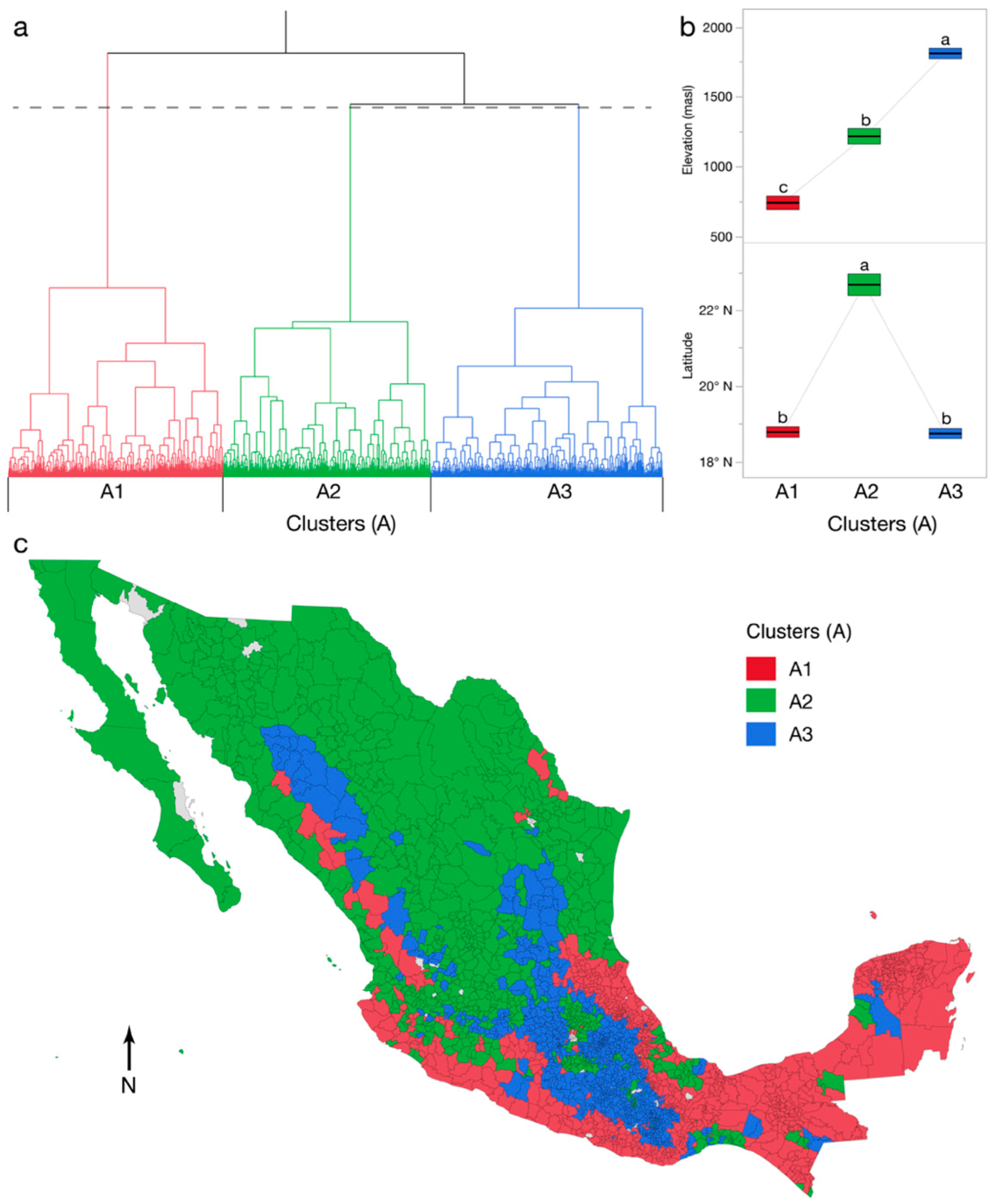
The HAC analysis identified a set of three clusters as optimal for minimizing intra-cluster variance and maximizing inter-cluster separation (CCC = 18.81). These clusters (A1–A3) are illustrated in the HAC dendrogram (Figure 1a) and are mapped (Figure 1c). Differences in latitude and elevation (higher-order distinctions) are illustrated graphically (Figure 1b). Based on these distinctions, geographical classifications were used to distinguish the three cluster types: southern lowlands (A1), northern midlands (A2), and south-central highlands (A3). The sharp elevation distinctions among types were similar to those of a previous typology study of southern Mexico [15]. Beyond this, lower-order differences in farm characteristics and cropping patterns were added to the geographical classifications, which led to the following typology descriptions.
A1. Southern lowland, low-input farms (n = 791). Of the 2412 municipalities considered for analysis, 791 were classified as southern lowland farm types (Table 2). This type had the highest rates of hand tool use (73%), commercial and financial challenges to production (64% and 27%, respectively), and the highest % of farm members belonging to an indigenous community (31%). This type also had the lowest rates of mechanized labor and draft animal use (8% and 5%, respectively), and the lowest irrigation and chemical fertilizer land ratios (8% and 6%, respectively). The cropping patterns of A1 showed by far the highest share of coffee (16%) and pasture grasses (14%) cultivation. About 47% of cropland was cultivated with maize, which was just under the national average of 52% (Table 1). The A1 type also had the lowest share of lands cultivated with beans (4%). None of the other 20 crops comprised more than 1% of cultivated lands (Table 2).
A2. Northern irrigated, commercial farms (n = 765). This type had the highest rates of mechanized labor (68%), by far the largest share of croplands receiving irrigation (36%). The A2 type had relatively high rates of commercial (63%) and financial (24%) challenges to production and chemical fertilizer use (35%). The type also had the lowest rates of subsistence production (47%) and membership from indigenous communities (1%) by far, and also the lowest % of farms experiencing climatic factors as a primary challenge to production (68%). The A2 type had the highest share of croplands cultivated with sorghum (for food = 8%; for forage = 5%), sugar (6%), forage alfalfa (6%), forage oats (5%), and wheat (4%). However, the A2 type had by far the smallest share of croplands cultivated with maize (28%) and coffee (0%), two of the most dominant crops nationally.
A3. Highland maize-based subsistence farms (n = 856). Through comprising the smallest geographical area, municipalities of this farm type were most common. The A3 type had the highest rates of subsistence production (87%), chemical fertilizer land use (45%), draft animal use (39%), and climate-related challenges to production (84%). The A3 type also had the lowest rates identifying commercial (38%) or financial (14%) challenges to production, but the largest shares of croplands dedicated to cultivation of maize (75%) and beans (3%). After maize and beans, none of the other 20 most dominant crops nationally comprised more than 3% of the cultivated area among type A3 municipalities.
3.3. B Clusters (n = 12)
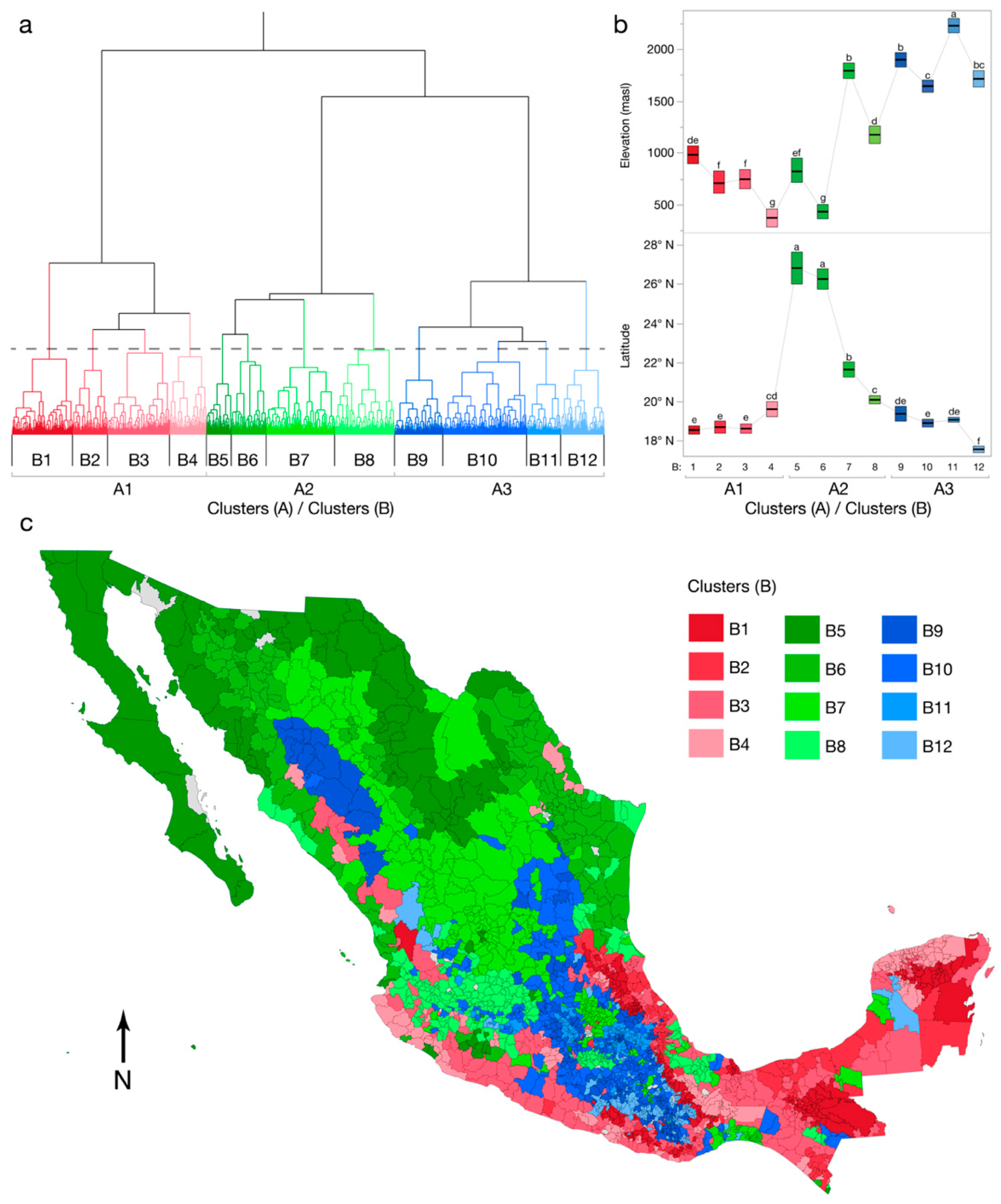
The HAC analysis also identified a set of 12 clusters that provided excellent statistical fit (CCC = 9.06). These were termed B clusters and represented B sub-groups within the A clusters group (i.e., A1 [B1–B4], A2 [B5–B8], A3 [B9–B12]). To emphasize this hierarchy, each B cluster was represented by a different shade of red (B1–B4), green (B5–B8), and blue (B9–B12) (Figure 2a–c) following the color scheme of type A.
The differences in latitude and elevation observed among A clusters also were observed among B clusters, though significant differences in the northern midland farm type (A2) emerged (Figure 2b). While clusters B1–B4 and B9–B10 retained their general distinctions in latitude, elevation classifications were somewhat less distinct than in type A. The B5 and B6 clusters were classified as northern and northern-lowland farm types, respectively, while B7 and B8 as central-highland and southern-midland farm types, respectively. Using these and other main distinctions from Figure 2 and Table 3 and used to qualitatively describe type B clusters below.
Typology B (1–12):
- B1. Southern coffee farms, indigenous labor using hand tools for subsistence (n = 247)
- B2. Southern coffee & sugar farms facing commercial challenges (n = 139)
- B3. Southern, non-descript coffee & grassland farms (n = 254)
- B4. Southern-lowland grassland farms facing financial challenges (n = 151)
- B5. Northern irrigated & mechanized, wheat & alfalfa, financial challenges (n = 101)
- B6. Northern lowland & mechanized, irrigated forage crops (n = 141)
- B7. Central highland & mechanized, beans, forage oats & alfalfa, & wheat (n = 280)
- B8. Southern midland, sugar & sorghum, high inputs & commercial challenges (n = 243)
- B9. Highland maize/beans subsistence, draft animals, climate ch. & chem.fertz. (n = 198)
- B10. Southern highland, maize/beans subsistence (n = 341)
- B11. Southern highland, maize, chemical fertz. & climate challenges (n = 138)
- B12. Southern highland, indigenous, subsistence maize/beans (n = 179)
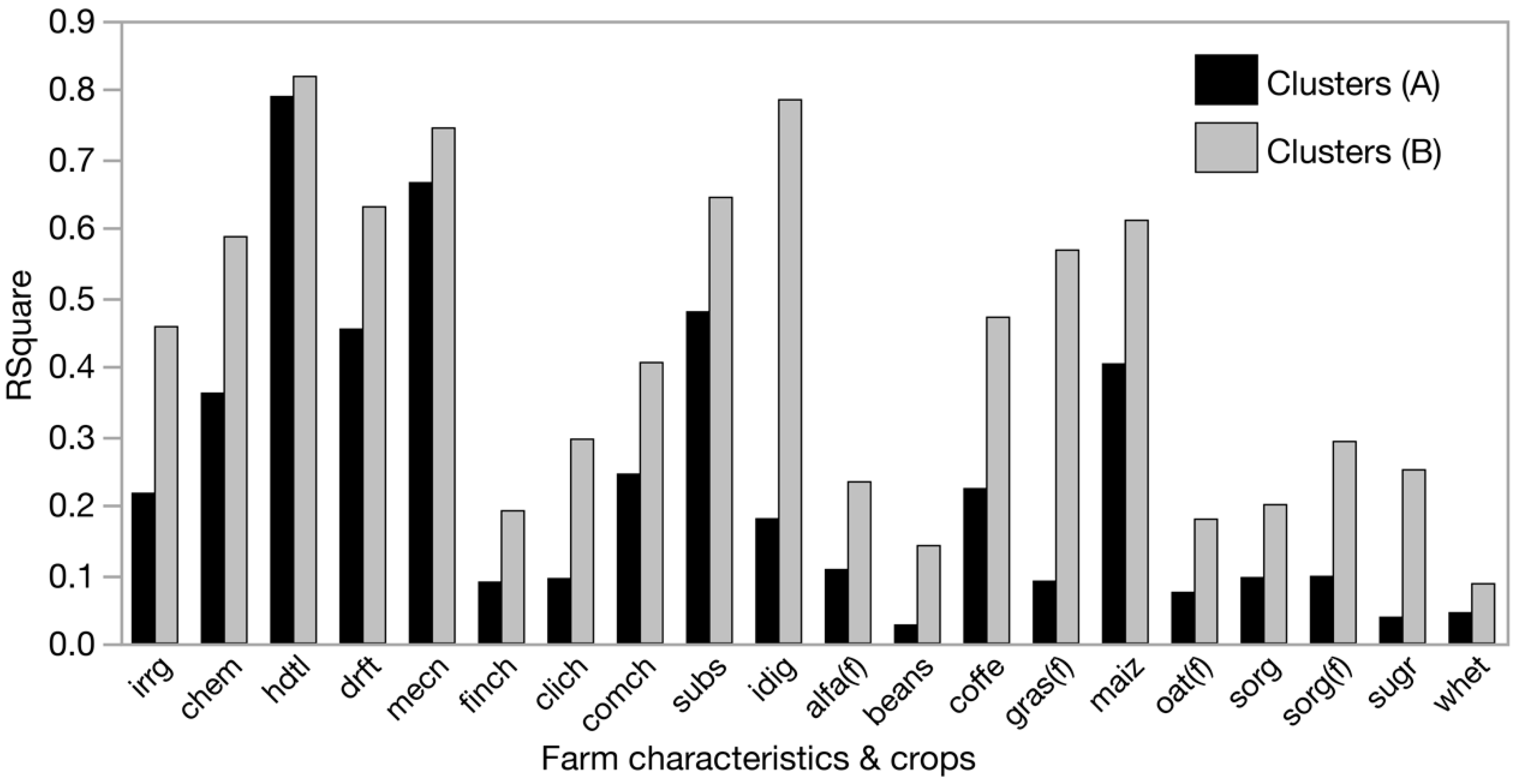
Though both cluster groups showed excellent separation based on the CCC statistic, the B clusters group showed greater lower-order separation of clusters by municipality farm characteristics and cropping patterns (Table 3; Figure 3). Individually, each of these 20 variables also explained a greater proportion of cluster variance in typology B than in typology A (Figure 4). Among those explaining the greater shares, in both typologies were those representing forms of farm labor and the % subsistence production and chemical fertilizer land use variables. The two variables with the largest differences in r-square between A and B typologies were the % of farm members from an indigenous community (r-square = 0.18 [A] and 0.79 [B]) and in the % of the cultivated area with forage grasses (r-square = 0.08 [A] and 0.58 [B]).
3.4. Multiple Correspondence Analysis (MCA)
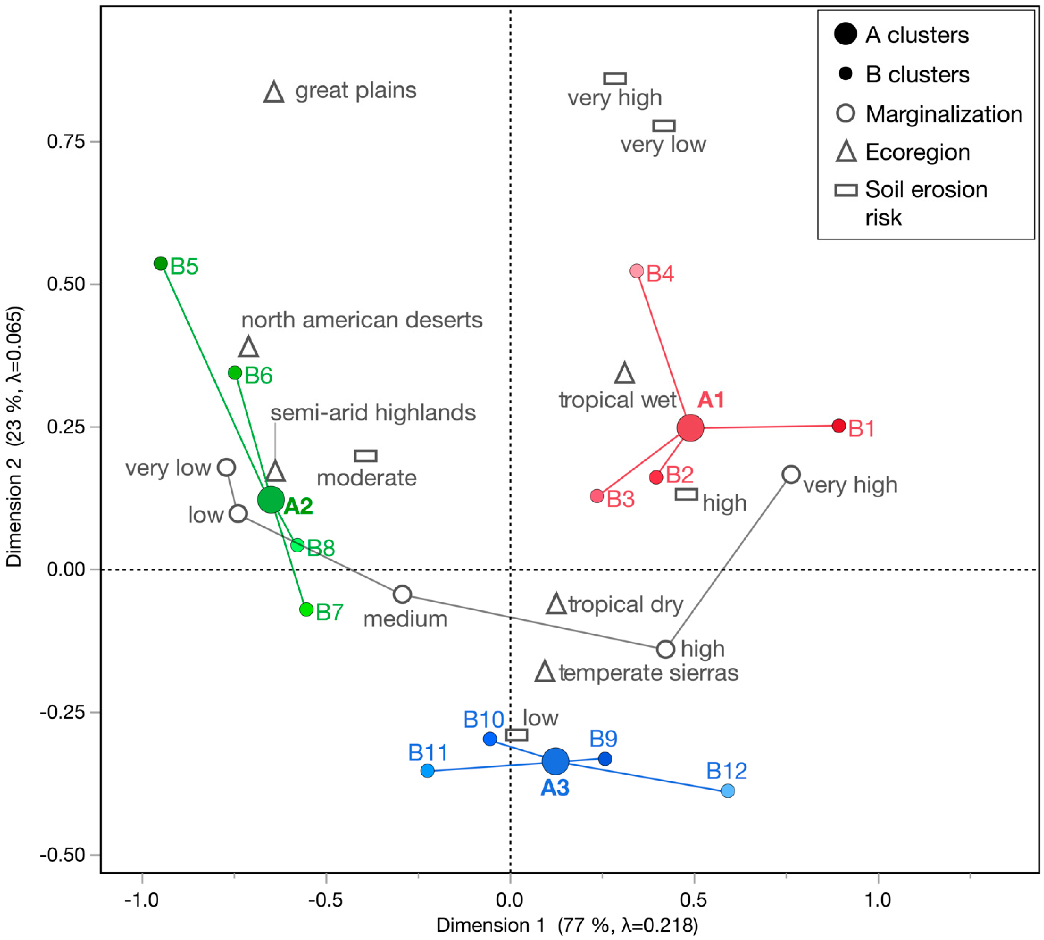
In Figure 5, the MCA correspondence plot illustrates associations among: (1) farm type clusters A, (2) marginality, and (3) water erosion risk; and the supplementary variables: (4) farm type clusters B and (5) ecoregion. In part, due to the simplified, three-level typology A, two dimensions alone explained 100% of the total inertia (λ = 0.28) found in the multivariate relationships. The good separation between the A-cluster groups identified in the HAC analysis (i.e., CCC = 18.81) was reflected in the MCA by the strong spatial separation among A cluster, where each occupied a different quadrant.
Dimension 1 accounted for the lion’s share of total inertia (77%) and Dimension 2, the remainder (23%). Dimension 1 primarily distinguished cluster types A1 and A3, and their negative association was illustrated visually by the horizontal distances between points A1 and A3 in Figure 5, and strong partial contributions of A1 and A3 to the total inertia of Dimension 1 (Table A1). Dimension 2 primarily distinguished cluster types A3 and A1, this time illustrated as the vertical distances between points A3 and A1 in Figure 5 and the partial contributions of A3 and A1 to the total inertia of Dimension 2 (Table A1).
Dimension 1 tracked closely with marginalization level. The categorical levels of marginalization moved in an ordinal sequence across Dimension 1, increasing from left to right. The plot of marginalization was less influenced by Dimension 2, which nonetheless modified the ordinal sequence and formed a U-shaped pattern reflecting a ‘Guttman effect’ [50,51]. Cluster A2 was closely associated with very low and low marginalization, while Cluster A1 was closely associated with very high and high marginalization. Among B-level clusters, the strongest contrast in marginality level was between Cluster B1 (red) and B5 or B6 (green), which also reflected strong geographical separation from South to North (Figure 2b,c).
Dimension 2 tracked more closely with soil erosion risk, which also contributed a greater share of the total inertia of the dimension (Table A1). Along this axis, cluster A1 was closely associated with high erosion risk, cluster A3 with low erosion risk, and cluster A2 with moderate erosion risk. Interestingly, the two extreme values, very low and very high erosion risk, were weakly associated with any cluster. The two supplementary variables provided additional context for interpretation and discussion. For example, cluster A1 was closely associated with the tropical wet ecoregion, while cluster A3 with the temperate sierras. Cluster A2 was closely associated with the North American deserts and semi-arid highlands ecoregions. The geographical associations between these ecoregions and the typology maps in this study (Figure 1c and Figure 2c) were consistent, which provides additional context for discussion.
4. Discussion
This study constructed two national-level farm typologies (A and B) of farm structural and functional characteristics and cropping patterns in Mexico. The typologies were comprised of a series of clusters that were classified and validated using statistical approaches and qualitative descriptions (Objective 1). A brief example used MCA to demonstrate how the typologies could be used by scaling organizations to target policy interventions (Objective 2). Below is a discussion of each typology, its relationship to existing conceptualizations of farm regions in Mexico, and how the typologies can be used in combination to facilitate targeting at larger (type A) and smaller (type B) spatial scales.
4.1. Farm Typology A: Higher-Order Distinctions for General Applications
The analysis found typology A provided excellent statistical separation between cluster groups (CCC = 18.81)—even though it divided the diverse characteristics of 2412 municipalities into only three clusters. This was surprising given the heterogeneity of agricultural landscapes in Mexico and the diversity of attributes selected for analysis. However, the six-step validation and description of these clusters revealed distinctions that broadly aligned with characterizations from existing studies.
For example, the southern lowland farm type (A1) was characterized by low farm inputs, high use of hand tools, high levels of subsistence production, and a high percent of farm members from indigenous groups. Cropping patterns were characterized by the dominance of maize, coffee, and forage grasses. These findings are consistent with many regional studies of southern Mexico, which highlight tensions between the subsistence-based livelihoods in the region and the cash-based coffee farms, which contribute little to subsistence production [52,53]. In this region, studies also find some of the highest marginalization (poverty) rates in the country [54]. These and more general characterizations of the region were confirmed by the A1 typology characterization in this study, and by its associations with other variables in the MCA.
The northern commercial farm type (A2) contrasted sharply with the A1 type. Again, the main features revealed in this study confirmed regional characterizations from existing studies. Intensive commercial agriculture dominates much of northern Mexico, where irrigation rates are among the highest in the country [55,56,57]. In northern regions, intensive irrigation and mechanization drive the production of a broad diversity of crops, including multiple forage crops, fruit and vegetable species, and ornamental plants, largely for export to the United States [47,58,59]. Though wealth is unevenly distributed, the northern farm regions have some of the lowest levels of marginalization (poverty) in the country—characterizations again confirmed by typology A and its associations in the MCA.
The highland farm type (A3) reflected many attributes of traditional agricultural systems in Mexico. Agriculture in highland regions is often characterized by maize-bean subsistence and the dependence on draft animals [60,61,62]. These characteristics broadly reflect the smallholder, maize-based intercropping (milpa) systems so prevalent in highland regions [63,64]. The relatively high levels of chemical fertilizers used in this farming region [65] and the high vulnerability of production to climatic shocks [66,67,68] were also confirmed by the typologies.
Though a simplification of the heterogeneity of agricultural landscapes across the country, typology A served two important purposes. First, it provides an important framework for understanding key distinctions in the agricultural geography of Mexico. These include: (1) higher-order, geographical distinctions in latitude and elevation, (2) distinctions between the northern, commercial agricultural systems in proximity of the U.S. borderlands and the southern, subsistence-based systems near the indigenous heartlands of Mesoamerica. Typology A also revealed several important lower-order distinctions between farm types related to farm labor attributes, challenges to production, levels of access to irrigation, and specific cropping patterns.
The second main purpose of typology A was to provide an appropriate starting point along the scaling pathway for targeting national-level policies. Once focused on the appropriate region, interventions can then be further targeted toward the lower-order characteristics of type B municipalities and eventually, tailored to match farm-level needs.
4.2. Farm Typology B: Lower-Order Distinctions for Precision Targeting
The analysis found typology B also provided excellent statistical separation between cluster groups (CCC = 9.06), but divided municipalities into 12 clusters. Though some of the higher-order distinctions identified in type A clusters (e.g., elevation, latitude) were also present in the type B sub-groups, the strong statistical association broke down among the 12 clusters. This made qualitative characterization of typology B more challenging. Nonetheless, the key distinctions between type B clusters improved model specificity and potentially provided greater targeting precision.
Several variables played prominent roles in distinguishing type B clusters. Among these, the % of farms with members of an indigenous community showed the largest increase in r-squared from type A to type B. The variable explained only 18% of cluster variance in typology A, but about 79% in typology B. This was also reflected in sharp means separation among of the variable among B types, which were 70% and 68% in B1 and B12, but less than 23% among all other B types. As a municipality-level variable, the % of indigenous community membership has been a priority criterion for other agricultural support programs in Mexico [15,24]. Two other key variables for targeting agricultural interventions were also among those with the largest increases in r-square from type A to type B: % cultivated land with irrigation and with chemical fertilizers. Together, as key targeting criteria, the large share of cluster variance explained by these three variables suggests that typology B would provide an appropriate framework for targeting policies where these variables represented priority criteria.
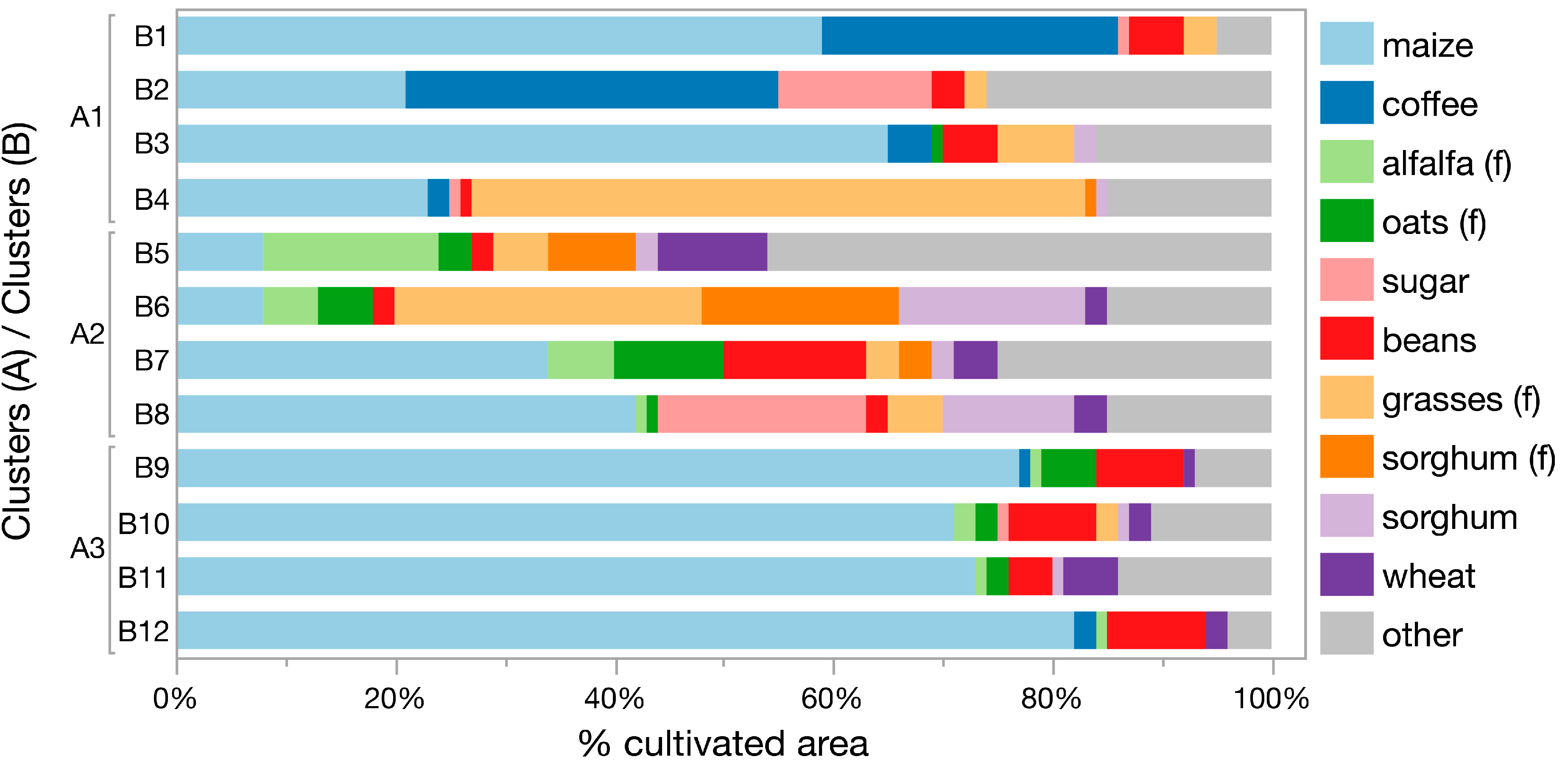
The cropping pattern distinctions that emerged in typology B also draw interesting comparisons with existing research. The cropping patterns in type B also illustrate important distinctions between the three type A regions. For example, the A2 farm type group exhibited the highest crop species diversity in typology A. Here, the mean % cultivated area for the 20 dominant crops was less skewed toward any one crop (evenness diversity), and further, less-dominant crop species (i.e., “other” crops) comprised a greater share of the total cultivated area (Table 2). Though a less reliable indicator of crop species diversity than the many diversity indices provide, it nonetheless confirms recent findings from such indices identifying northern irrigated regions with some of the highest crop species richness and evenness diversity in the country [47]. Further, once stratified into clusters B4-B8, the cropping patterns with this set of municipalities continue to diversify into different cropping patters (Figure 3).
In sharp contrast, the highland farm type (A3) exhibited a cropping pattern skewed towards maize and beans. Further, the A3 type had the smallest share of farmland dedicated to growing less dominant (i.e., “other) crops (Table 2). Interestingly, once stratified in B9-B12 clusters this basic cropping pattern largely remained, exhibiting a more homogenous pattern among the B9–B12 set of municipalities. The pattern strongly reflected the maize-based milpa systems of the central Mexican highlands. While crop genetic diversity (especially maize) can be exceedingly high in milpa systems [69,70]; the crop species compositions in municipalities of these farm regions tend to be more homogenous than among the A2 (B5–B8) regions [47].
In sum, while the higher-order distinctions between type A groups provide a framework for identifying three basic farm type regions, the type B group provides a more appropriate framework for targeting policy interventions. An optimal clustering solution is one that: (1) achieves good separation between clusters, (2) explains a high proportion of variances, and (3) provides a level of hierarchical agglomeration that suits the purpose of the inquiry. Here, both A and B typologies met these criteria in different ways.
4.3. Typology-Based Targeting of Agricultural Interventions
The MCA results show municipalities of the A1 type should be prioritized for soil erosion interventions due to the close associations with high marginality and soil erosion risk. Subgroups of the A1 type, B1 and B2, showed even closer association with the criteria. The B1 type included 247 municipalities with farm types characterized as southern, maize and coffee producing farms with strong indigenous populations, who primarily use hand tools and are engaged in subsistence production. The B2 type included 139 municipalities that were similar to the B1 type but tended to have smaller share of farm members from indigenous communities, higher rates of sugar cultivation, lower rates of maize cultivation, and a greater % of farms facing financial and commercial challenges to production.
At this early stage of the scaling process, the MCA serves two main purposes. First, it helps identify farm types most closely associated with the priority criteria. Second, it provides additional context and validation for these relationships. Supplementary variables primarily serve the second purpose. For example, the A1 farm type and high soil erosion risk categories were also associated with the tropical wet ecoregion. In Mexico, this ecoregion experiences some of the western hemisphere’s highest precipitation rates [71] and most frequent and severe landslides [72]. Agricultural soil and water management in the region is a primary driver of land degradation, agricultural production, and several forms of vulnerability [73]. In sum, existing research on agricultural soil management and erosion risk in the tropical wet ecoregion supports the prioritization of A1 farm type for soil erosion interventions. By incorporating the supplementary variables, the MCA served not only to target A1 farm regions, but to provide critical context for validating this decision.
Additional refinement of the targeting strategy can be made by further examination of the lower-order variables represented in the typology. For example, after identifying the A1 farm type group, policymakers could then target interventions based on secondary criteria. In this case, subsistence level, % use of hand tools, and % indigenous population feature prominently. Additionally, the targeting of soil erosion interventions to the A1 type has potential to generate spillover effects that address food security (subsistence production), to provide short-term employment for farm laborers (high % hand tool use), and to provide assistance to indigenous communities (high % indigenous membership). Indeed, these general priority criteria are found in several existing policy directives in Mexico [74,75,76].
In sum, targeting farms of based on types rather than singular criteria alone allows policy makers to address multiple policy objectives at once; or, to assess the potential for spillover or synergistic effects on other farm system attributes. As this study has shown, MCA offers one potential tool for targeting farm type regions during early stages of the scaling pathway.
4.4. Limitations and Future Study
This study had several limitations. First, the methodology relied on statistical and descriptive approaches instead of participatory approaches. In part, this was a consequence of the scale of analysis, which employed large-scale census and crop production data. In addition, variable selection relied on previous research and data availability rather than the participation and input of farmers or local experts. Numerous studies show participatory approaches can play important roles in typology formation that can strongly influence results [10,17,18,77]. Therefore, the results of this study should be interpreted with this in mind. Relatedly, this study also adopted more of an exploratory approach than one driven primarily by hypothesis testing—though the latter has potential to reduce subjectivity in typology formation [14].
The statistical approaches chosen also introduced limitations. HAC was selected over other clustering techniques due to the exploratory nature of the inquiry (i.e., the number of clusters was not predetermined). However, other clustering methods could potentially produce different results. Further, determining the optimal number of clusters is a recurring challenge of cluster analyses. Indeed, in this study several other possible cluster solutions provided CCC measures similar to that of the 12-cluster, type B solution. Additional research is needed to explore whether other clustering solutions would have provided significantly different results. Future work also should explore in greater detail the spatial dimensions of the farm types/regions identified in this study. This includes quantifying the spatial clustering of municipalities by typology into statistically significant hot spots. Such analysis would help strengthen the links between the characteristics-based farm typology clusters and their clustering into spatially distinct farm regions.
Finally, the targeting example used in the MCA was a simplified version of what such an effort would likely entail. Inclusion of additional variables would have better reflected the diversity of policy objectives and selection criteria often involved in policy targeting efforts in Mexico. Nonetheless, the simplified example effectively illustrated how a typology-based targeting approach would work. Future research is needed to explore the limits of the approach in applied situations.
5. Conclusions
This study made two contributions to agricultural geography, systems research, and policy. First, it developed two national-level typologies of farm regions in Mexico. Importantly, these farm regions conceptualizations were based not only on biophysical parameters but on statistical groupings of farm-level structural and functional characteristics and cropping patterns. This organization provides better representation of the diversity inherent in Mexican agricultural systems than do one-dimensional soils or ecoregions maps. Accounting for this diversity is essential if agricultural policies are to effectively address the increasingly broad set of policy objectives. These objectives are now associated not only with food and fiber production, but with environmental, rural development, energy, and sustainability concerns.
Second, this study demonstrated how such typologies can serve as actionable tools for targeting policy interventions. Hierarchical agglomerative cluster analysis was used to construct the typologies, and multiple correspondence analysis was used to illustrate relationships between the typologies and the selection criteria for interventions. The typologies allowed for different levels of targeting specificity—Typology A (3 farm classes) was defined more by higher-order geographical distinctions (i.e., latitude and elevation), while typology B (12 farm classes) primarily revealed lower-order relationships between farm characteristics and cropping patterns. Together, both typologies were used to identify municipalities that best corresponded with the selection criteria for interventions. This included municipalities of the southern, lowland farm type (A1) and, more specifically, municipalities of two smaller subtypes (B1 and B12).
Funding
This research received no external funding.
Institutional Review Board Statement
Not applicable.
Data Availability Statement
All data are publicly available.
Acknowledgments
Sandra Nashif made helpful comments on an early draft of this paper. Two anonymous reviewers also provided helpful comments and suggestions on a later draft.
Conflicts of Interest
The author declares no conflict of interest.
Appendix A

Table A1.
Partial variable contributions to inertia for each MCA dimension.
| Partial Contributions to Inertia | ||||
|---|---|---|---|---|
| Position | Variable | Category | Dimension 1 | Dimension 2 |
| row (X) | cluster (A) | 1 | 0.36 | 0.31 |
| 2 | 0.61 | 0.07 | ||
| 3 | 0.03 | 0.62 | ||
| column (Y) | marginalization | very low | 0.14 | 0.03 |
| low | 0.22 | 0.01 | ||
| medium | 0.04 | 0.00 | ||
| high | 0.15 | 0.06 | ||
| very high | 0.20 | 0.03 | ||
| soil erosion risk | very low | 0.06 | 0.39 | |
| low | 0.00 | 0.35 | ||
| moderate | 0.10 | 0.09 | ||
| high | 0.09 | 0.02 | ||
| very high | 0.00 | 0.02 | ||
References
- Sinha, A.; Basu, D.; Priyadarshi, P.; Ghosh, A.; Sohane, R.K. Farm Typology for Targeting Extension Interventions Among Smallholders in Tribal Villages in Jharkhand State of India. Front. Environ. Sci. 2022, 10, 823338. [Google Scholar] [CrossRef]
- Cervantes-Jiménez, M.; Mastachi-Loza, C.A.; Díaz-Delgado, C.; Gómez-Albores, M.Á.; González-Sosa, E. Socio-Ecological Regionalization of the Urban Sub-Basins in Mexico. Water 2017, 9, 14. [Google Scholar] [CrossRef]
- OECD. Evaluation of Agricultural Policy Reforms in the United States; OECD: Paris, France, 2011; ISBN 978-92-64-09671-4. [Google Scholar]
- Abler, D. Multifunctionality, Agricultural Policy, and Environmental Policy. Agric. Resour. Econ. Rev. 2004, 33, 8–17. [Google Scholar] [CrossRef]
- Arovuori, K.; Kola, J. Multifunctional Policy Measures for Multifunctional Agriculture. Available online: https://ageconsearch.umn.edu/record/24771 (accessed on 5 July 2020).
- Dibden, J.; Cocklin, C. ‘Multifunctionality’: Trade Protectionism or a New Way Forward? Environ. Plan. A 2009, 41, 163–182. [Google Scholar] [CrossRef]
- Bernués, A.; Alfnes, F.; Clemetsen, M.; Eik, L.O.; Faccioni, G.; Ramanzin, M.; Ripoll-Bosch, R.; Rodríguez-Ortega, T.; Sturaro, E. Exploring Social Preferences for Ecosystem Services of Multifunctional Agriculture across Policy Scenarios. Ecosyst. Serv. 2019, 39, 101002. [Google Scholar] [CrossRef]
- Kuivanen, K.S.; Alvarez, S.; Michalscheck, M.; Adjei-Nsiah, S.; Descheemaeker, K.; Mellon-Bedi, S.; Groot, J.C.J. Characterising the Diversity of Smallholder Farming Systems and Their Constraints and Opportunities for Innovation: A Case Study from the Northern Region, Ghana. NJAS Wagening. J. Life Sci. 2016, 78, 153–166. [Google Scholar] [CrossRef]
- Bartkowski, B.; Schüßler, C.; Müller, B. Typologies of European Farmers: Approaches, Methods and Research Gaps. Reg. Environ. Chang. 2022, 22, 43. [Google Scholar] [CrossRef]
- Tittonell, P.; Bruzzone, O.; Solano-Hernández, A.; López-Ridaura, S.; Easdale, M.H. Functional Farm Household Typologies through Archetypal Responses to Disturbances. Agric. Syst. 2020, 178, 102714. [Google Scholar] [CrossRef]
- Graskemper, V.; Yu, X.; Feil, J.-H. Farmer Typology and Implications for Policy Design—An Unsupervised Machine Learning Approach. Land Use Policy 2021, 103, 105328. [Google Scholar] [CrossRef]
- Nyambo, D.G.; Luhanga, E.T.; Yonah, Z.Q. A Review of Characterization Approaches for Smallholder Farmers: Towards Predictive Farm Typologies. Sci. World J. 2019, 2019, e6121467. [Google Scholar] [CrossRef] [Green Version]
- Hammond, J.; Rosenblum, N.; Breseman, D.; Gorman, L.; Manners, R.; van Wijk, M.T.; Sibomana, M.; Remans, R.; Vanlauwe, B.; Schut, M. Towards Actionable Farm Typologies: Scaling Adoption of Agricultural Inputs in Rwanda. Agric. Syst. 2020, 183, 102857. [Google Scholar] [CrossRef]
- Alvarez, S.; Timler, C.J.; Michalscheck, M.; Paas, W.; Descheemaeker, K.; Tittonell, P.; Andersson, J.A.; Groot, J.C.J. Capturing Farm Diversity with Hypothesis-Based Typologies: An Innovative Methodological Framework for Farming System Typology Development. PLoS ONE 2018, 13, e0194757. [Google Scholar] [CrossRef] [PubMed]
- LaFevor, M.C.; Frake, A.N.; Couturier, S. Targeting Irrigation Expansion to Address Sustainable Development Objectives: A Regional Farm Typology Approach. Water 2021, 13, 2393. [Google Scholar] [CrossRef]
- Musafiri, C.M.; Macharia, J.M.; Ng’etich, O.K.; Kiboi, M.N.; Okeyo, J.; Shisanya, C.A.; Okwuosa, E.A.; Mugendi, D.N.; Ngetich, F.K. Farming Systems’ Typologies Analysis to Inform Agricultural Greenhouse Gas Emissions Potential from Smallholder Rain-Fed Farms in Kenya. Sci. Afr. 2020, 8, e00458. [Google Scholar] [CrossRef]
- Teixeira, H.M.; Van den Berg, L.; Cardoso, I.M.; Vermue, A.J.; Bianchi, F.J.J.A.; Peña-Claros, M.; Tittonell, P. Understanding Farm Diversity to Promote Agroecological Transitions. Sustainability 2018, 10, 4337. [Google Scholar] [CrossRef]
- Kuivanen, K.S.; Michalscheck, M.; Descheemaeker, K.; Adjei-Nsiah, S.; Mellon-Bedi, S.; Groot, J.C.J.; Alvarez, S. A Comparison of Statistical and Participatory Clustering of Smallholder Farming Systems—A Case Study in Northern Ghana. J. Rural. Stud. 2016, 45, 184–198. [Google Scholar] [CrossRef]
- Righi, E.; Dogliotti, S.; Stefanini, F.M.; Pacini, G.C. Capturing Farm Diversity at Regional Level to Up-Scale Farm Level Impact Assessment of Sustainable Development Options. Agric. Ecosyst. Environ. 2011, 142, 63–74. [Google Scholar] [CrossRef]
- Carletto, C.; Jolliffe, D.; Banerjee, R. From Tragedy to Renaissance: Improving Agricultural Data for Better Policies. J. Dev. Stud. 2015, 51, 133–148. [Google Scholar] [CrossRef]
- Daskalopoulou, I.; Petrou, A. Utilising a Farm Typology to Identify Potential Adopters of Alternative Farming Activities in Greek Agriculture. J. Rural. Stud. 2002, 18, 95–103. [Google Scholar] [CrossRef]
- Jerven, M. Poor Numbers: How We Are Misled by African Development Statistics and What to Do about It; Cornell University Press: Ithaca, NY, USA, 2013; ISBN 978-0-8014-6761-5. [Google Scholar]
- Randall, A. Monitoring Sustainability and Targeting Interventions: Indicators, Planetary Boundaries, Benefits and Costs. Sustainability 2021, 13, 3181. [Google Scholar] [CrossRef]
- LaFevor, M.C.; Ponette-González, A.G.; Larson, R.; Mungai, L.M. Spatial Targeting of Agricultural Support Measures: Indicator-Based Assessment of Coverages and Leakages. Land 2021, 10, 740. [Google Scholar] [CrossRef]
- Kansiime, M.K.; van Asten, P.; Sneyers, K. Farm Diversity and Resource Use Efficiency: Targeting Agricultural Policy Interventions in East Africa Farming Systems. NJAS Wagening. J. Life Sci. 2018, 85, 32–41. [Google Scholar] [CrossRef]
- Hoppe, R.A.; MacDonald, J.M. Updating the ERS Farm Typology; U.S. Department of Agriculture, Economic Research Service: Washginton, DC, USA, 2013; p. 40.
- Johnson, J. A Typology for U.S. Farms from National Survey Data. In Proceedings of the Workshop on the Farm Household-Firm Unit: Its Importance in Agriculture and Implications for Statistics (No. 15725); International Agricultural Policy Reform and Adjustment Project (IAPRAP), London, UK, 12 April 2002; p. 18. [Google Scholar]
- Sommer, J.E.; Hines, F.K. Diversity in US Agriculture: A New Delineation by Farming Characteristics; U.S. Department of Agriculture, Economic Research Service, Agriculture and Rural Economy Division: Washington, DC, USA, 1991; p. 23.
- Hammond Wagner, C.R.; Niles, M.T.; Roy, E.D. US County-Level Agricultural Crop Production Typology. BMC Res. Notes 2019, 12, 552. [Google Scholar] [CrossRef]
- Wade, T.; Claassen, R.; Wallander, S. Conservation-Practice Adoption Rates Vary Widely by Crop and Region; U.S. Department of Agriculture, Economic Research Service: Washington, DC, USA, 2015; p. 40.
- Ehlers, M.-H.; Huber, R.; Finger, R. Agricultural Policy in the Era of Digitalisation. Food Policy 2021, 100, 102019. [Google Scholar] [CrossRef]
- Song, B.; Robinson, G.M. Multifunctional Agriculture: Policies and Implementation in China. Geogr. Compass 2020, 14, e12538. [Google Scholar] [CrossRef]
- National Academies of Sciences, Engineering and Medicine. Improving Data Collection and Measurement of Complex Farms; Kling, C., Mackie, C., Eds.; National Academies Press: Washington, DC, USA, 2019; ISBN 0-309-48460-X. [Google Scholar]
- Aguilar, J.; Gramig, G.G.; Hendrickson, J.R.; Archer, D.W.; Forcella, F.; Liebig, M.A. Crop Species Diversity Changes in the United States: 1978–2012. PLoS ONE 2015, 10, e0136580. [Google Scholar] [CrossRef]
- Contreras Servin, C.; Galindo Mendoza, M.G.; Ibarra Zapata, E. Las Regiones Agroecológicas de México. In Proceedings of the XIX Reunión Nacional SELPER-México Memorias; Centro de Investigaciones en Geografía Ambiental (CIGA): Morelia, Michoacån, Mexico, 18 February 2012; Volume Memorias SELPER. pp. 122–126. [Google Scholar]
- Arroyo, G. Regiones Agrícolas de México: Modernización Agrícola, Heterogeneidad Estructural y Autosuficiencia Alimentaria. In Balance y Perspectivas de los Estudios Regionales en México; CIIH-UNAM; M.A. Porrúa Grupo Editorial: Mexico City, Mexico, 1990; pp. 147–222. [Google Scholar]
- SIAP Anuario Estadístico de La Producción Agrícola. Available online: https://nube.siap.gob.mx/cierreagricola/ (accessed on 8 May 2022).
- INEGI, I.N. de E. y Mapas. Uso de Suelo y Vegetación. Available online: https://www.inegi.org.mx/temas/usosuelo/ (accessed on 10 July 2022).
- CAP. Censo Agrícola, Ganadero y Forestal 2007 (Censo Agropecuario); Instituto Nacional de Estadística y Geografía (INEGI): Mexico City, Mexico, 2008.
- INEGI (Instituto Nacional de Estadística y Geografía). El VIII Censo Agrícola, Ganadero y Forestal 2007: Aspectors Metodológicos y Principales Resultados. Available online: https://www.inegi.org.mx/programas/cagf/2007/ (accessed on 27 March 2020).
- Murtagh, F.; Contreras, P. Algorithms for Hierarchical Clustering: An Overview. WIREs Data Min. Knowl. Discov. 2012, 2, 86–97. [Google Scholar] [CrossRef]
- SAS. SAS Help Center: Cubic Clustering Criterion. Available online: https://documentation.sas.com/doc/en/emref/14.3/n1dm4owbc3ka5jn11yjkod7ov1va.htm (accessed on 11 July 2022).
- Rodriguez-Sabate, C.; Morales, I.; Sanchez, A.; Rodriguez, M. The Multiple Correspondence Analysis Method and Brain Functional Connectivity: Its Application to the Study of the Non-Linear Relationships of Motor Cortex and Basal Ganglia. Front Neurosci. 2017, 11, 345. [Google Scholar] [CrossRef]
- CONAPO. Indice de Marginación Por Município 2005; Comisión Nacional de Población: Mexico City, Mexico, 2020.
- UACh, S.-C. SEMARNAT Evaluación de La Degradación Del Suelo Causada Por El Hombre En La República Mexicana, Escala 1: 250,000. SEMARNAT. In Memoria Nacional SEMARNAT-Colegio de Posgraduados; SEMARNAT: Mexico City, Mexico, 2002. [Google Scholar]
- CONABIO. Ecorregiones Terrestres de México. Available online: https://www.biodiversidad.gob.mx/region/ecorregiones (accessed on 26 July 2022).
- LaFevor, M.C.; Pitts, A.K. Irrigation Increases Crop Species Diversity in Low-Diversity Farm Regions of Mexico. Agriculture 2022, 12, 911. [Google Scholar] [CrossRef]
- Zahniser, S.; López, N.F.L.; Motamed, M.; Vargas, Z.Y.S.; Capehart, T. The Growing Corn Economies of Mexico and the United States. In US Department of Agriculture, Economic Research Service, FDS-19f-01; USDA: Washington, DC, USA, 2019. [Google Scholar]
- Lerner, A.M.; Appendini, K. Dimensions of Peri-Urban Maize Production in the Toluca-Atlacomulco Valley, Mexico. J. Lat. Am. Geogr. 2011, 10, 87–106. [Google Scholar] [CrossRef]
- García-Ochoa, R.; Avila-Ortega, D.I.; Cravioto, J. Energy Services’ Access Deprivation in Mexico: A Geographic, Climatic and Social Perspective. Energy Policy 2022, 164, 112822. [Google Scholar] [CrossRef]
- Johs, H. Multiple Correspondence Analysis for The Social Sciences, 1st ed.; Routledge: Abingdon, UK; New York, NY, USA, 2018; ISBN 978-1-315-51625-7. [Google Scholar]
- Fernandez, M.; Méndez, V.E. Subsistence under the Canopy: Agrobiodiversity’s Contributions to Food and Nutrition Security amongst Coffee Communities in Chiapas, Mexico. Agroecol. Sustain. Food Syst. 2019, 43, 579–601. [Google Scholar] [CrossRef]
- Aguilar-Støen, M.; Angelsen, A.; Stølen, K.-A.; Moe, S.R. The Emergence, Persistence, and Current Challenges of Coffee Forest Gardens: A Case Study From Candelaria Loxicha, Oaxaca, Mexico. Soc. Nat. Resour. 2011, 24, 1235–1251. [Google Scholar] [CrossRef]
- Bellon, M.R.; Hodson, D.; Bergvinson, D.; Beck, D.; Martinez-Romero, E.; Montoya, Y. Targeting Agricultural Research to Benefit Poor Farmers: Relating Poverty Mapping to Maize Environments in Mexico. Food Policy 2005, 30, 476–492. [Google Scholar] [CrossRef]
- Arreguín-Cortes, F.I.A.; Villanueva, N.H.G.; Casillas, A.G.; Gonzalez, J.A.G. Reforms in the Administration of Irrigation Systems: Mexican Experiences. Irrig. Drain. 2019, 68, 6–19. [Google Scholar] [CrossRef]
- Cerutti, M. The Agriculturization of the Desert. State, Irrigation, and Agriculture in Northern Mexico (1925–1970). Apuntes 2015, 42, 91. [Google Scholar] [CrossRef]
- Moreno, T.A.; Huber-Sannwald, E. Impacts of Drought on Agriculture in Northern Mexico. In Coping with Global Environmental Change, Disasters and Security; Brauch, H.G., Oswald Spring, Ú., Mesjasz, C., Grin, J., Kameri-Mbote, P., Chourou, B., Dunay, P., Birkmann, J., Eds.; Hexagon Series on Human and Environmental Security and Peace; Springer: Berlin/Heidelberg, Germany, 2011; Volume 5, pp. 875–891. ISBN 978-3-642-17775-0. [Google Scholar]
- LaFevor, M.C. Spatial and Temporal Changes in Crop Species Production Diversity in Mexico (1980–2020). Agriculture 2022, 12, 985. [Google Scholar] [CrossRef]
- Hartman, S.; Chiarelli, D.D.; Rulli, M.C.; D’Odorico, P. A Growing Produce Bubble: United States Produce Tied to Mexico’s Unsustainable Agricultural Water Use. Environ. Res. Lett. 2021, 16, 105008. [Google Scholar] [CrossRef]
- Rogé, P.; Astier, M. Changes in Climate, Crops, and Tradition: Cajete Maize and the Rainfed Farming Systems of Oaxaca, Mexico. Hum. Ecol. 2015, 43, 639–653. [Google Scholar] [CrossRef]
- Arnés, E.; Antonio, J.; del Val, E.; Astier, M. Sustainability and Climate Variability in Low-Input Peasant Maize Systems in the Central Mexican Highlands. Agric. Ecosyst. Environ. 2013, 181, 195–205. [Google Scholar] [CrossRef]
- González-Amaro, R.M.; Martínez-Bernal, A.; Basurto-Peña, F.; Vibrans, H. Crop and Non-Crop Productivity in a Traditional Maize Agroecosystem of the Highland of Mexico. J. Ethnobiol. Ethnomedicine 2009, 5, 38. [Google Scholar] [CrossRef]
- Novotny, I.P.; Tittonell, P.; Fuentes-Ponce, M.H.; López-Ridaura, S.; Rossing, W.A.H. The Importance of the Traditional Milpa in Food Security and Nutritional Self-Sufficiency in the Highlands of Oaxaca, Mexico. PLoS ONE 2021, 16, e0246281. [Google Scholar] [CrossRef]
- Moreno-Espíndola, I.P.; Ferrara-Guerrero, M.J.; Luna-Guido, M.L.; Ramírez-Villanueva, D.A.; De León-Lorenzana, A.S.; Gómez-Acata, S.; González-Terreros, E.; Ramírez-Barajas, B.; Navarro-Noya, Y.E.; Sánchez-Rodríguez, L.M.; et al. The Bacterial Community Structure and Microbial Activity in a Traditional Organic Milpa Farming System under Different Soil Moisture Conditions. Front. Microbiol. 2018, 9, 2737. [Google Scholar] [CrossRef]
- LaFevor, M.C.; Magliocca, N.R. Farmland Size, Chemical Fertilizers, and Irrigation Management Effects on Maize and Wheat Yield in Mexico. J. Land Use Sci. 2020, 15, 532–546. [Google Scholar] [CrossRef]
- Osuna-Ceja, E.S.; Pimentel-López, J.; Padilla-Ramírez, J.S.; Martínez-Gamiño, M.Á.; Figueroa-Sandoval, B.; Osuna-Ceja, E.S.; Pimentel-López, J.; Padilla-Ramírez, J.S.; Martínez-Gamiño, M.Á.; Figueroa-Sandoval, B. The Sustainability and Resilience of a Rainfed Agroforestry System for the Semi-Arid Highlands of Mexico. Rev. Mex. De Cienc. Agrícolas 2019, 10, 63–75. [Google Scholar] [CrossRef]
- Peralta-Hernández, A.R.; Barba-Martínez, L.R. The Risk of Early and Late Frost Behavior in Central México under El Niño Conditions. Atmósfera 2009, 22, 111–123. [Google Scholar]
- Eakin, H. Institutional Change, Climate Risk, and Rural Vulnerability: Cases from Central Mexico. World Dev. 2005, 33, 1923–1938. [Google Scholar] [CrossRef]
- Heindorf, C.; Reyes–Agüero, J.A.; van’t Hooft, A.; Fortanelli–Martínez, J. Inter- and Intraspecific Edible Plant Diversity of the Tének Milpa Fields in Mexico. Econ. Bot. 2019, 73, 489–504. [Google Scholar] [CrossRef]
- Birol, E.; Villalba, E.R.; Smale, M. Farmer Preferences for Milpa Diversity and Genetically Modified Maize in Mexico: A Latent Class Approach. Environ. Dev. Econ. 2009, 14, 521–540. [Google Scholar] [CrossRef]
- de Anda Sánchez, J. Precipitation in Mexico. In Water Resources of Mexico; Raynal-Villasenor, J.A., Ed.; World Water Resources; Springer International Publishing: Cham, Switzerland, 2020; pp. 1–14. ISBN 978-3-030-40686-8. [Google Scholar]
- Díaz, S.R.; Cadena, E.; Adame, S.; Dávila, N. Landslides in Mexico: Their Occurrence and Social Impact since 1935. Landslides 2020, 17, 379–394. [Google Scholar] [CrossRef]
- Zúñiga, E.; Magaña, V. Vulnerability and Risk to Intense Rainfall in Mexico: The Effect of Land Use Cover Change. Investig. Geográficas 2018, 95, 1–18. [Google Scholar] [CrossRef]
- DOF. Programa Nacional Hidrico, 2020-2024; Diario Oficial de la Federación (DOF): Cuauhtémoc, Mexico, 2020.
- FAO-SAGARPA. Informe de Evaluación de Consistencia y Resultados 2007: Programa Integral de Agricultural Sostenible y Reconversión Productiva En Zonas de Siniestralidad Recurrente (PIASRE); SAGARPA-CONZA: Mexico City, Mexico, 2008; p. 155.
- SAGARPA. DOF—Diario Oficial de La Federación: CRITERIOS de Distribución de Recursos a Las Entidades Federativas Para El Programa Integral de Agricultura Sostenible y Reconversión Productiva En Zonas de Siniestralidad Recurrente en El Marco del PIASRE 2006. SAGARPA. México, Distrito Federal, MX. 2006. Available online: http://diariooficial.gob.mx/nota_detalle.php?codigo=2119832&fecha=02/03/2006#gsc.tab=0 (accessed on 11 July 2022).
- Hammond, J.; van Wijk, M.T.; Smajgl, A.; Ward, J.; Pagella, T.; Xu, J.; Su, Y.; Yi, Z.; Harrison, R.D. Farm Types and Farmer Motivations to Adapt: Implications for Design of Sustainable Agricultural Interventions in the Rubber Plantations of South West China. Agric. Syst. 2017, 154, 1–12. [Google Scholar] [CrossRef] [Green Version]
Figure 1.
(a) Dendrogram of cluster (A) solution (CCC = 18.81). (b) Differences in mean elevation and latitude shown with 95% means confidence intervals with different letters representing statistical significance as determined by Kruskal–Wallace and Dunn’s post hoc tests. (c) Mapped clusters, with omitted municipalities shaded gray.

Figure 2.
(a) Dendrogram of 12-cluster (B) solution (CCC = 9.06). (b) Differences in elevation and latitude with different letters (a–g) indicating statistical significance as determined by Kruskal–Wallace and Dunn’s post hoc tests. (c) Mapped clusters with omitted municipalities shaded gray.
Figure 2.
(a) Dendrogram of 12-cluster (B) solution (CCC = 9.06). (b) Differences in elevation and latitude with different letters (a–g) indicating statistical significance as determined by Kruskal–Wallace and Dunn’s post hoc tests. (c) Mapped clusters with omitted municipalities shaded gray.

Figure 3.
Mean % of cultivated area with each crop per cluster (B1–B12).

Figure 4.
The proportion of the variance explained by each variable per cluster group (A and B).

Figure 5.
Correspondence plot for Clusters (A) (row), marginalization level (column) and soil erosion risk level (column). Clusters (B) and ecoregion are supplementary variables.
Figure 5.
Correspondence plot for Clusters (A) (row), marginalization level (column) and soil erosion risk level (column). Clusters (B) and ecoregion are supplementary variables.

Table 1.
Descriptive characteristics of variables.
| Municipalities (N = 2455) | |||||||||
|---|---|---|---|---|---|---|---|---|---|
| 25th | 75th | ||||||||
| Category | Type | Variable | Code | Unit | Pctile | Median | Pctile | Mean | SD |
| farm | land use | irrigation | irrg | % cropland | 0.01 | 0.07 | 0.28 | 0.19 | 0.25 |
| characteristics | chemical fertz. | chem | 0.04 | 0.21 | 0.50 | 0.29 | 0.27 | ||
| labor | hand tools | hdtl | % farms | 0.01 | 0.10 | 0.60 | 0.29 | 0.35 | |
| draft animals | drft | 0.01 | 0.09 | 0.28 | 0.19 | 0.23 | |||
| mechanization | mecn | 0.02 | 0.22 | 0.58 | 0.32 | 0.31 | |||
| challenges | financial chall. | finch | 0.06 | 0.16 | 0.32 | 0.22 | 0.20 | ||
| climate chall. | clich | 0.62 | 0.82 | 0.93 | 0.75 | 0.23 | |||
| commercial chall. | comch | 0.36 | 0.55 | 0.74 | 0.54 | 0.25 | |||
| socioeconomic | subsistence | subs | 0.57 | 0.80 | 0.93 | 0.72 | 0.25 | ||
| indigenous | indig | 0.00 | 0.01 | 0.22 | 0.17 | 0.28 | |||
| crops | alfalfa (forage) | alfa(f) | % cropland | 0.00 | 0.00 | 0.00 | 0.02 | 0.07 | |
| beans | beans | 0.00 | 0.01 | 0.07 | 0.06 | 0.10 | |||
| coffee | coffe | 0.00 | 0.00 | 0.00 | 0.05 | 0.16 | |||
| grasses (forage) | gras(f) | 0.00 | 0.00 | 0.03 | 0.08 | 0.19 | |||
| maize | maiz | 0.25 | 0.53 | 0.78 | 0.51 | 0.30 | |||
| oats (forage) | oat(f) | 0.00 | 0.00 | 0.01 | 0.03 | 0.08 | |||
| sorghum | sorg | 0.00 | 0.00 | 0.00 | 0.03 | 0.11 | |||
| sorghum (forage) | sorg(f) | 0.00 | 0.00 | 0.00 | 0.02 | 0.08 | |||
| sugar | sugr | 0.00 | 0.00 | 0.00 | 0.03 | 0.12 | |||
| wheat | whet | 0.00 | 0.00 | 0.00 | 0.02 | 0.08 | |||
Table 2.
Variable means in each cluster (A), shaded by ordered rank, with highest (bold), middle (italics), and lowest (none) values.
Table 2.
Variable means in each cluster (A), shaded by ordered rank, with highest (bold), middle (italics), and lowest (none) values.
| Clusters | Mun | Farm Characteristics (%) | |||||||||
|---|---|---|---|---|---|---|---|---|---|---|---|
| A | No. | Irrg | Chem | Hdtl | Drft | Mecn | Finch | Clich | Comch | Subs | Indig |
| A1 | 791 | 0.08 | 0.06 | 0.73 | 0.05 | 0.08 | 0.27 | 0.71 | 0.64 | 0.81 | 0.31 |
| A2 | 765 | 0.36 | 0.35 | 0.07 | 0.09 | 0.68 | 0.24 | 0.68 | 0.63 | 0.47 | 0.01 |
| A3 | 856 | 0.15 | 0.45 | 0.09 | 0.39 | 0.22 | 0.14 | 0.84 | 0.38 | 0.87 | 0.18 |
| Crops (% Cultivated Area) | |||||||||||
| alfa(f) | beans | coffe | gras(f) | maiz | oat(f) | sorg | sorg(f) | sugr | whet | ||
| A1 | 791 | 0.00 | 0.04 | 0.16 | 0.14 | 0.47 | 0.00 | 0.01 | 0.00 | 0.03 | 0.00 |
| A2 | 765 | 0.06 | 0.06 | 0.00 | 0.09 | 0.28 | 0.05 | 0.08 | 0.05 | 0.06 | 0.04 |
| A3 | 856 | 0.01 | 0.07 | 0.01 | 0.01 | 0.75 | 0.02 | 0.01 | 0.00 | 0.00 | 0.02 |
Table 3.
Variable means in each cluster (B), shaded by ordered rank and highest (bold), second highest (italics), and third highest (gray-none) values—see Table 1 for explanation of variable codes.
Table 3.
Variable means in each cluster (B), shaded by ordered rank and highest (bold), second highest (italics), and third highest (gray-none) values—see Table 1 for explanation of variable codes.
| Clusters | Mun. | Farm Characteristics (%) | ||||||||||
|---|---|---|---|---|---|---|---|---|---|---|---|---|
| A | B | No. | Irrg | Chem | Hdtl | Drft | Mecn | Finch | Clich | Comch | Subs | Indig |
| A1 | B1 | 247 | 0.02 | 0.02 | 0.85 | 0.05 | 0.01 | 0.17 | 0.85 | 0.62 | 0.92 | 0.70 |
| B2 | 139 | 0.02 | 0.09 | 0.72 | 0.04 | 0.08 | 0.32 | 0.71 | 0.81 | 0.71 | 0.10 | |
| B3 | 254 | 0.07 | 0.09 | 0.66 | 0.08 | 0.12 | 0.31 | 0.65 | 0.57 | 0.81 | 0.10 | |
| B4 | 151 | 0.25 | 0.06 | 0.68 | 0.04 | 0.12 | 0.33 | 0.58 | 0.63 | 0.71 | 0.22 | |
| A2 | B5 | 101 | 0.81 | 0.38 | 0.04 | 0.05 | 0.72 | 0.38 | 0.58 | 0.75 | 0.29 | 0.01 |
| B6 | 141 | 0.39 | 0.15 | 0.03 | 0.06 | 0.74 | 0.24 | 0.70 | 0.46 | 0.26 | 0.01 | |
| B7 | 280 | 0.23 | 0.23 | 0.03 | 0.13 | 0.68 | 0.15 | 0.85 | 0.54 | 0.63 | 0.02 | |
| B8 | 243 | 0.30 | 0.59 | 0.13 | 0.09 | 0.62 | 0.30 | 0.50 | 0.78 | 0.50 | 0.01 | |
| A3 | B9 | 198 | 0.07 | 0.50 | 0.09 | 0.58 | 0.08 | 0.10 | 0.87 | 0.29 | 0.92 | 0.08 |
| B10 | 341 | 0.25 | 0.35 | 0.08 | 0.28 | 0.26 | 0.18 | 0.80 | 0.45 | 0.82 | 0.05 | |
| B11 | 138 | 0.09 | 0.73 | 0.02 | 0.18 | 0.46 | 0.14 | 0.88 | 0.44 | 0.85 | 0.02 | |
| B12 | 179 | 0.08 | 0.37 | 0.17 | 0.54 | 0.10 | 0.11 | 0.84 | 0.28 | 0.94 | 0.68 | |
| Crops (% cultivated area) | ||||||||||||
| alfa(f) | beans | coffe | gras(f) | maíz | oat(f) | sorg | sorg(f) | sugr | whet | |||
| A1 | B1 | 247 | 0.00 | 0.05 | 0.27 | 0.03 | 0.59 | 0.00 | 0.00 | 0.00 | 0.01 | 0.00 |
| B2 | 139 | 0.00 | 0.03 | 0.34 | 0.02 | 0.21 | 0.00 | 0.00 | 0.00 | 0.14 | 0.00 | |
| B3 | 254 | 0.00 | 0.05 | 0.04 | 0.07 | 0.65 | 0.01 | 0.02 | 0.00 | 0.00 | 0.00 | |
| B4 | 151 | 0.00 | 0.01 | 0.02 | 0.56 | 0.23 | 0.00 | 0.01 | 0.01 | 0.01 | 0.00 | |
| A2 | B5 | 101 | 0.16 | 0.02 | 0.00 | 0.05 | 0.08 | 0.03 | 0.02 | 0.08 | 0.00 | 0.10 |
| B6 | 141 | 0.05 | 0.02 | 0.00 | 0.28 | 0.08 | 0.05 | 0.17 | 0.18 | 0.00 | 0.02 | |
| B7 | 280 | 0.06 | 0.13 | 0.00 | 0.03 | 0.34 | 0.10 | 0.02 | 0.03 | 0.00 | 0.04 | |
| B8 | 243 | 0.01 | 0.02 | 0.00 | 0.05 | 0.42 | 0.01 | 0.12 | 0.00 | 0.19 | 0.03 | |
| A3 | B9 | 198 | 0.01 | 0.08 | 0.01 | 0.00 | 0.77 | 0.05 | 0.00 | 0.00 | 0.00 | 0.01 |
| B10 | 341 | 0.02 | 0.08 | 0.00 | 0.02 | 0.71 | 0.02 | 0.01 | 0.00 | 0.01 | 0.02 | |
| B11 | 138 | 0.01 | 0.04 | 0.00 | 0.00 | 0.73 | 0.02 | 0.01 | 0.00 | 0.00 | 0.05 | |
| B12 | 179 | 0.01 | 0.09 | 0.02 | 0.00 | 0.82 | 0.00 | 0.00 | 0.00 | 0.00 | 0.02 | |
Publisher’s Note: MDPI stays neutral with regard to jurisdictional claims in published maps and institutional affiliations. |
© 2022 by the author. Licensee MDPI, Basel, Switzerland. This article is an open access article distributed under the terms and conditions of the Creative Commons Attribution (CC BY) license (https://creativecommons.org/licenses/by/4.0/).
Share and Cite
MDPI and ACS Style
LaFevor, M.C. Characterizing Agricultural Diversity with Policy-Relevant Farm Typologies in Mexico. Agriculture 2022, 12, 1315. https://doi.org/10.3390/agriculture12091315
AMA Style
LaFevor MC. Characterizing Agricultural Diversity with Policy-Relevant Farm Typologies in Mexico. Agriculture. 2022; 12(9):1315. https://doi.org/10.3390/agriculture12091315
Chicago/Turabian StyleLaFevor, Matthew C. 2022. "Characterizing Agricultural Diversity with Policy-Relevant Farm Typologies in Mexico" Agriculture 12, no. 9: 1315. https://doi.org/10.3390/agriculture12091315
Note that from the first issue of 2016, this journal uses article numbers instead of page numbers. See further details here.