Consequences of Ignoring Dependent Error Components and Heterogeneity in a Stochastic Frontier Model: An Application to Rice Producers in Northern Thailand

Abstract

The traditional Stochastic Frontier Model (SFM) suffers from a very restrictive assumption of independence of its error components and also limited ability to address heterogeneity (inefficiency effects) satisfactorily, thereby leading to potential biases in the estimation of model parameters, identification of inefficiency effect variables influencing efficiency and, ultimately, efficiency scores. This paper aims to investigate the consequences of ignoring any dependency in error components and heterogeneity in the stochastic frontier model, and proposes a copula-based SFM with heterogeneity to resolve such weaknesses based on a simulation study to prove its superiority over the traditional SFM, followed by an empirical application on a sample of rice producers from northern Thailand. We demonstrate that the proposed model, i.e., copula-based SFM with dependent error components and heterogeneity, is unbiased and robust. The simulation experiments show that the traditional SFM can cause biases in parameter estimation and severe overestimation of technical efficiency. The traditional SFM with heterogeneity also has similar consequences. However, just ignoring heterogeneity does not have a great impact on parameter estimation and technical efficiency compared to the consequence of ignoring dependency in error components. The empirical application of the proposed model results show that land, labor and material inputs are all significant drivers of rice production in our copula-based SFM with dependent error components and heterogeneity, whereas in the traditional SFM model only the land variable seems to be a significant driver of rice production. The mean technical efficiency (MTE) score was also overestimated by two points in the traditional SFM, i.e., MTE = 0.88 versus 0.86. Finally, results of the copula-based SFM with dependent error components and heterogeneity reveals that both subsistence pressure and the use of hired labor are significantly associated with technical inefficiency, whereas the traditional SFM could identify the effect of hired labor use only. Therefore, caution is necessary when interpreting results from the conventional SFM as the results may be biased, incomplete and/or inadequate.

1. Introduction

The parametric route of productivity and efficiency analysis using the production frontier framework has come a long way from deterministic frontier analysis using Ordinary Least Squares (OLS) regression [1] to Corrected Ordinary Least Squares (COLS) regression [2]. After the Stochastic Frontier Model (SFM) was proposed independently by Aigner et al. [3] and Meeusen and Van den Broeck [4], which was a breakthrough and by far the most popular. since then, stochastic frontier models have been applied to analyze technical efficiency [5,6,7], cost efficiency [8,9], energy efficiency [10], trade potential [11], and total factor productivity [9,12,13] etc. Therefore, the stochastic frontier model has been used extensively, and applied in various fields.

The SFM is essentially a linear regression model with two error components: a two-sided term that captures random variation of the production frontier across firms (i.e., a conventional random error, $\mathrm{v}$) and a one-sided term that measures inefficiency relative to the frontier (i.e., the inefficiency component, $\mathrm{w}$). The key assumption in the SFM is the independence between the inefficiency component and the random error term. Some scholars have relaxed this assumption in SFM by using copula functions. For example, Smith [14] first proposed an SFM allowing for dependence between the two error components using copula functions, which can be used to capture rank correlation and tail dependence between these two error components, thus lifting the restrictive assumption of independence between the inefficiency component and the random error. Mehdi and Hafner [15] proposed a bootstrap algorithm to estimate the copula-based SFM. Wiboonpongse et al. [16] proposed a simulated maximum likelihood method (SMLE), which has numerical and computational advantages over the numerical integration method used by Smith [14]. Since the structure of the dependence of the two error components is unknown, Wiboonpongse et al. [16] systematically considered a number of copula families, such as Student-t, Clayton, Gumbel and Joe families, including their relevant rotated versions, to select the best fit model based on established and well-known AIC and BIC criteria. Bonanno et al. [17] further considered asymmetry of random error as the basis of dependent error components. Similarly, Amsler et al. [18] applied copula to measure time dependence in stochastic frontier model, and Lai and Kumbhakar [19] measured the dependence between the time-varying and time-invariant components. Wei et al. [20] constructed an asymmetric dependence in the stochastic frontier model using skew normal copula.

Based on the above literature, we see that the copula-based SFM has been widely applied and extended. However, the consequences of the assumption of independence of error components remain unclear. It is also not clear if when the inefficiency effect (i.e., heterogeneity) is absent in the copula-based SFM, the parameter and efficiency estimates remain correct. In addition, which limitation is more serious, the assumption of independence of error components or missing heterogeneity? Therefore, the main motivation of this paper is to clarify the consequence of missing inefficiency effects and/or ignoring dependency in error components in the copula-based SFM. The contribution of this study are three-fold. First, we adopt the approach proposed by Wiboonpongse et al. [16] and Sriboochitta [21] and extend it further by developing a model to jointly estimate the copula-based SFM along with heterogeneity in a single stage, as done by Battese and Coelli [22] for the conventional SFM, which is a new contribution to the existing literature on productivity and efficiency analysis. In addition, the consequences arising from the independence assumption of error components and the lack of heterogeneity are fully revealed and interpreted, respectively. Then, we apply this framework to a sample of 300 rice farmers from northern Thailand and demonstrate relative merit of the copula based SFM as compared to the conventional SFM with respect to estimation efficiency of the parameters of the production frontier and the inefficiency effects functions, estimates of the mean technical efficiency scores, distribution of the technical efficiency scores and shift in the relative ranking of the individual farmers between the two models.

The rest of the paper is organized as follows. Section 2 introduces the family of copula functions considered in this study to select the best fit model. Section 3 presents the structure of the copula-based stochastic frontier model. Section 4 presents the empirical results. Section 5 concludes and draws policy implications.

2. Methodology

Since the analytical approach is based on the use of copula functions, we first introduce the various copula families that are relevant in the process of searching the best fit model. Next we introduce the structure of the copula-based SFM used in this study.

2.1. Copulas and Dependence

A copula connects a given number of marginal distributions (one-dimensional distributions) to form a joint (multivariate) distribution [23,24]. If given a joint distribution H, then the copula function C can be expressed by

$$H(x_1,x_2)=H(F_1{}^{-1}(u_1),F_2{}^{-1}(u_2))=C(F_1(x_1),F_2(x_2);\theta )$$

(1)

where $u_1=F_1(x_1)$ and $u_2=F_2(x_2)$, $\theta$ is a parameter vector of the copula commonly referred to as the dependence parameter vector, F₁(.) and F₂(.) are marginal distributions (see [25,26,27,28]).

In addition, Sklar’s theorem [29] shows that any multivariate probability distribution function can be represented with a marginal distribution and a dependent structure, which is derived below:

$$\begin{array}{l}f(x_1,\cdots \cdots ,x_n)=\frac{\partial F(x_1,\cdots \cdots ,x_n)}{\partial x_1\cdots \partial x_n}\\ =\frac{\partial C(u_1,\cdots ,u_n)}{\partial u_1\cdots \partial u_n}\times \prod \frac{\partial F(x_i)}{\partial x_i}\\ =c(u_1,\cdots ,u_n)\times \prod f_i(x_i)\end{array}$$

(2)

So, a bivariate density function of x₁ and x₂ can be decomposed into marginal densities and copula density as well, $f(x_1,x_2)=c(u_1,u_2)f_1(x_1)f_2(x_2)$.

The most common method to measure dependence is Pearson’s linear correlation which, however, does not have information for asymmetric distributions [28,30]. Therefore, the limitations of Pearson’s linear correlation led us to use rank correlations that are Kendall’s τ and Spearman’s ρ to measure nonlinear dependence expressed as follows:

$${\tau }_{X_1{X}_2}=4\underset{0}{\overset{1}{{\displaystyle \iint }}}C\left(u_1,u_2\right)dC\left(u_1,u_2\right)-1=4E\left[C\left(U_1,U_2\right)\right]-1$$

(3)

$$\begin{gathered} S_{\rho \left(X_1{X}_2\right)}=12\underset{0}{\overset{1}{{\displaystyle \iint }}}{u}_1{u}_{2}dC\left(u_1,u_2\right)-3=12\underset{0}{\overset{1}{{\displaystyle \iint }}}C\left(u_1,u_2\right)d{u}_1{u}_2-3 \\ =12E\left[C\left(U_1,U_2\right)\right]-3 \end{gathered}$$

(4)

In addition to nonlinear dependence, a copula function can also be used to measure tail dependence. Tail dependence describes the limiting proportion that one margin exceeds a certain threshold when the other margin has already exceeded that threshold [31]. Once the SFM fits well and the composite error is small, but both the inefficiency term and the random error are large, there may exist upper tail dependence between error components. When the estimated technical efficiency scores are high (low) and the random error is small (large), there may exist positive (negative) lower tail dependence between error components. Most copulas can capture upper tail and/or lower tail dependences. For instance, the Clayton copula can measure lower tail dependence, and Gumbel copula and Joe copula families can measure upper tail dependence, while the Student-t copula can measure symmetric tail dependence [32,33]. However, these copulas can only capture positive dependence except for the Gaussian, T copula and Frank copula. Fortunately, these copulas may then be ‘rotated’ and applied again. There are three rotated forms: rotated 90 degrees, rotated 180 degrees and rotated 270 degrees. When rotating them by 180 degrees, one obtains the corresponding survival copulas. The non-rotated Clayton copula can capture lower tail dependence, while the survival Clayton copula can measure upper tail dependence. Rotation by 90 and 270 degrees allow for modelling of negative dependence (for details of rotated copulas, please see [32,34,35]). The distribution functions of rotated copulas by 90, 180 and 270 degrees are given as follows:

$$C_{90}(u_1,u_2)=u_2-C(1-u_1,u_2),$$

(5)

$$C_{180}(u_1,u_2)=u_1+u_2-1+C(1-u_1,1-u_2),$$

(6)

$$C_{270}(u_1,u_2)=u_1-C(u_1,1-u_2).$$

(7)

Therefore, we can make use of some copula families that cover a large dependence as much as possible, such as the (rotated) Clayton, (rotated) Gumbel and (rotated) Joe copula families, which can represent both negative and positive dependences [21].

2.2. Copula-Based Stochastic Frontier Model with Heterogeneity

Consider the stochastic frontier model (SFM)

$$\begin{gathered} y_i=X\beta +{\epsilon }_i \\ {\epsilon }_i=v_i-w_i \end{gathered}$$

(8)

where i = 1, 2, …, N, y_i is the dependent variable, $X$ is a N × k matrix of explanatory variables, $\beta$ is a k × 1 vector of unknown parameters that need be estimated, $v_i$ is a random error, and $w_i$ represents non-negative unobservable random variables that represent technical inefficiency. w_i and v_i are independent, and are assumed to have truncated normal and normal distribution following Coelli [36] and Guo et al. [37], respectively. The technical inefficiency effect, $w_i$, can be determined by some covariates. The formula of a technical inefficiency effect can be expressed as

$$w_i=z\delta +e_i$$

(9)

where z represents a vector of possible determinants of the firm’s inefficiency, δ is a vector of unknown parameters to be estimated, and $e_i$ is $N(0,{\sigma }_w^2)$ truncated on the left at −zδ. Then, $w_i$ is N(zδ, ${\sigma }_w^2$) truncated on the left at zero [38].

The conventional SFM imposes a restrictive assumption that w_i and v_i are independent. Thus, we relax this independence assumption and allow copula to make optimum use of the stochastic frontier model. The copula-based SFM sufficiently regards dependence structure between w and v, using product copula. First, the density function of $f(w,v)$ can be transformed into $f(w,\epsilon )$ as follows:

$$f(w,v)=f(w,w+\epsilon )=f_W(w)\times f_V(w+\epsilon )\times c_{\theta }(F_W(w),F_V(w+\epsilon ))$$

(10)

Then, the probability density function of $\epsilon$ can be expressed as

$$f_{\theta }(\epsilon )={\displaystyle {\int }_{{\underset{\_}{R}}_{+}}f(w,\epsilon )}dw$$

or

$$f_{\Theta }(\epsilon )=E_W[f_V(W+\epsilon )c_{\theta }(F_W(W),F_V(W+\epsilon ))]$$

(11)

where $E_W[\cdot ]$ denotes the expected value pertaining to the distribution of technical inefficiency w. $\Theta$ represents all parameters that are from the regression equation, marginal and copula function. If the density function of ε exists in closed form, then the MLE method is suitable for estimating the copula-based SFM. Assume that we have cross-sectional observations of n individuals or firms. The likelihood function is then given by

$$L(\beta ,{\sigma }_w,{\sigma }_v,\delta ,\theta )={\displaystyle \prod _{i=1}^n{f}_{\Theta }}({\epsilon }_i)={\displaystyle \prod _{i=1}^n{f}_{\Theta }}(y_i-{x^{\prime }}_i\beta )$$

(12)

where $y_i$ is the output of individual $i$, $x_i$ is the vector of explanatory variable, and ${\sigma }_w$ and ${\sigma }_v$ are from the marginal distributions of $w$ and $v$, respectively. However, Smith [14] showed that there are very few density functions of $\epsilon$ for which the MLE has a closed form expression. Then, an alternative approach, the Simulated Maximum Likelihood Estimation method (SMLE), is used to estimate the unknown parameters of the copula-based SFM (for details, see [5,16,39,40]). Computation of the simulated log likelihood function requires that R draws from the corresponding distribution of w for each observation. If $w$ and v are assumed to have truncated normal and normal distributions, respectively, then the density function of $\epsilon$ can be shown as

$$f({\epsilon }_i)=\frac{1}{R}{\displaystyle \sum _{r=1}^R{f}_V(z_i\delta +e_{ir}+{\epsilon }_i)\times c_{\theta }(F_W(z_i\delta +e_{ir}),F_V(z_i\delta +e_{ir}+{\epsilon }_i))}$$

(13)

where ${\epsilon }_i=y_i-{\beta }^{\prime }{x}_i$, and R represents a large number draws. Let e_ir equal ${\sigma }_w\cdot {\Phi }^{-1}(\Phi (-z_i\delta /{\sigma }_w)+(1-\Phi (-z_i\delta /{\sigma }_w))\cdot P_{ir})$, where $P~U(0,1)$ is a uniform variable and $\Phi$ is cumulative normal distribution function. The simulated log-likelihood of the copula-based SFM can be expressed as follows:

$$L_s\left(\beta ,{\sigma }_w,{\sigma }_v,\delta ,\theta \right)\approx {\displaystyle \sum }_{i=1}^N\log \{\frac{1}{R}{\displaystyle \sum }_{r=1}^R{f}_V\left(z_i\delta +e_{ir}+{\epsilon }_i\right)c_{\theta }\left(F_W\left(z_i\delta +e_{ir}\right),F_V\left(z_i\delta +e_{ir}+{\epsilon }_i\right)\right)\}$$

(14)

In addition, following Battese and Coelli [22], the variance terms are parameterized by replacing the relevant parameters, λ, γ and ${\sigma }^2$, and be defined by $\lambda ={\sigma }_w/{\sigma }_v$, $\gamma ={\sigma }_w{}^2/({\sigma }_w{}^2+{\sigma }_v{}^2)$ and ${\sigma }^2={\sigma }_w{}^2+{\sigma }_v{}^2$. The larger λ, the greater the inefficiency component in the model [41,42]. Note that the standard errors of these parameters can be calculated by applying the invariance property.

The most important analysis of copula-based stochastic frontier model is the technical efficiency that is specified with

$$\begin{array}{c}T{E}_{\Theta }=E[\exp (-w)\left|\xi =\epsilon \right.]\hfill \\ =\frac{1}{f_{\Theta }(\epsilon )}{\displaystyle \underset{-z\delta }{\int }\exp (-z\delta -e)f(z\delta +e,\epsilon )}de\hfill \\ =\frac{E_e[\exp (-z\delta -e)f_V(z\delta +e+\epsilon )c_{\theta }(F_W(z\delta +e),F_V(z\delta +e+\epsilon ))]}{E_e[f_V(z\delta +e+\epsilon )c_{\theta }(F_W(z\delta +e),F_V(z\delta +e+\epsilon ))]}\hfill \\ \approx \frac{\frac{1}{R}{\displaystyle \sum _{r=1}^R\exp (-z_i\delta -e_{ir})\times f_V(z_i\delta +e_{ir}+{\epsilon }_i)\times c_{\theta }(F_W(z_i\delta +e_{ir}),F_V(z_i\delta +e_{ir}+{\epsilon }_i))}}{\frac{1}{R}{\displaystyle \sum _{r=1}^R{f}_V(z_i\delta +e_{ir}+{\epsilon }_i)\times c_{\theta }(F_W(z_i\delta +e_{ir}),F_V(z_i\delta +e_{ir}+{\epsilon }_i))}}\hfill \end{array}$$

(15)

Since the SMLE method is applied, the technical efficiency scores can be calculated by simulation as well. The models are estimated by a user-written program developed in R-software. Different copula families mean different SFMs. Therefore, model selection is very important. Following Joe [43], the AIC and BIC were used to select the best model in this study, and their formulas are expressed as follows:

$$\mathrm{AIC}=-2\mathrm{LogL}+2\ast \mathrm{k}$$

(16)

$$\mathrm{BIC}=-2\mathrm{LogL}+\mathrm{k}\ast \ln \left(\mathrm{N}\right)$$

(17)

3. Simulation Study

Is the simulated maximum likelihood estimation suitable for the copula-based stochastic frontier model with heterogeneity? What are consequences of ignoring dependent error components and/or heterogeneity in stochastic frontier model? To answer these questions, we performed a simulation experiment. Following the simulation experiments of Wei et al. [44], Liu et al. [45] and Zhu et al. [46], we randomly drew datasets from a copula-based stochastic frontier model with heterogeneity. The simulated process of this experiment can be illustrated as follows:

First, we set up the equation, $y_i=10+0.7x_i+v_i-w_i$, $w_i=0.7z_i+e_i$, where v_i is standard normal distributed. $w_i$ is N(0.7z_i, 1) truncated on the left at zero. The Kendall’s tau between two error components is assumed to be 0.6. The variables, x and z, are simulated from standard normal distribution, respectively. To check the impact of sample size on estimation, the sample size was set at 500, 1000 and 2000, respectively.

Second, we randomly drew numbers using Clayton copula corresponding to $\tau =0.6$, and obtained v and w by using the inverse functions. Thus, we could obtain y from the equation $y_i=10+0.7x_i+v_i-w_i$.

Third, we fixed R = 200 and maximized the simulated log-likelihood using the BFGS algorithm in the R statistical software for six models: the traditional SFM or copula-based SFM with the assumption of independence in error components (Model 1), the traditional SFM with heterogeneity or independent copula-based SFM with heterogeneity (Model 2), the Gaussian copula-based SFM with mis-specified dependent error components (Model 3), the Gaussian copula-based SFM with heterogeneity and mis-specified dependent error components (Model 4), the Clayton copula-based SFM (Model 5), and the Clayton copula-based SFM with heterogeneity and dependent error components (Model 6). Therefore, Model 1 ignores dependency of error components and heterogeneity. Thus, from the estimation of Model 1, we can see the impact of the traditional assumption of independent error components and homogeneity on parameter estimation. Model 2 is the traditional stochastic frontier with heterogeneity. Thus, the influence of assuming independent error components along with heterogeneity on parameter estimation can be found. We specify a wrong dependency structure between error components in Model 3 and Model 4. Then the simulation result can demonstrate that the consequence of the wrong specification of dependency structure. In Model 5, we correctly set the dependent error components but ignore heterogeneity. Therefore, the simulation results of the Model 5 can reflect the consequences of ignoring dependency in error components only. Finally, the simulation results of the Model 6 can demonstrate whether the proposed model is unbiased and robust.

Last, we randomly generated 100 datasets from Model 6 and estimated the parameters of Models 1–6. We then computed percent bias of the estimates and TE scores in all five models. On this basis, we also drew 100 datasets from Model 1, and used Model 6 to fit these datasets (opposite data) without heterogeneity and dependence. This simulation experiment can further illustrate whether the proposed model is more general.

Table 1. Percent bias of the six models (unit %). The smallest value is shown in bold.

N = 500	True	Model 1	Model 2	Model 3	Model 4	Model 5	Model 6	True	Model 6 (Opposite Data)
β0	10	−10.11	−6.77	−7.72	−3.92	−2.48	−0.30	10	−0.45
β1	0.7	−0.10	−0.07	−0.07	−0.03	−0.02	−0.02	0.7	−1.36
δ1	0.7		−36.85		−20.5		−1.85	0	−1.15
σw	1	−93.75	−85.99	−63.73	−49.01	2.74	−2.75	1	−5.36
σv	1	−26.95	−31.75	−15.79	−15.67	−15.67	1.89	1	−0.43
ρ	0.6			−16.38	−39.71	−5.22	1.10	0	0.91
	average	−32.73	−32.29	−20.74	−21.48	−4.17	−0.35		−1.31
	PAIC	0	0	0	0	0	100
N = 1000
β0	10	−10.38	−6.92	−8.05	−5.27	−2.26	−0.14	10	−0.56
β1	0.7	0.28	0.39	0.26	0.38	0.01	0.21	0.7	−0.22
δ1	0.7		−38.40		−26.19		−1.25	0	−12.59
σw	1	−97.43	−87.78	−68.22	−64.89	4.94	−1.27	1	−4.18
σv	1	−26.05	−30.92	−18.95	−21.49	−21.49	0.40	1	0.87
ρ	0.6			−22.04	−51.65	−7.80	−2.83	0	0.03
	average	−33.40	−32.73	−23.40	−28.18	−5.32	−0.81		−2.78
	PAIC	0	0	0	0	0	100
N = 2000
β0	10	−10.55	−6.95	−9.92	−4.58	−1.38	0.25	10	−0.22
β1	0.7	−0.12	−0.1	−0.12	−0.1	−0.22	−0.16	0.7	0.28
δ1	0.7		−38.11		−22.28		1.47	0	0.01
σw	1	−98.971	−87.80	−91.05	−56.72	16.44	3.24	1	2.96
σv	1	−25.46	−30.47	−23.71	−18.19	−18.19	0.73	1	0.76
ρ	0.6			−42.28	−45.26	−10.60	−0.13	0	0.03
	average	−33.77	−32.69	−33.42	−24.52	−2.79	0.90		0.64
	PAIC	0	0	0	0	0	100

Note: P_AIC denotes the proportion of the models selected by using AIC among 100 simulated data.

shows percent bias of Models 1–6. Model 6 is the best fit. The percentage of bias in estimates on average is the smallest of all the six models, and most of the estimates are the smallest as well, except β₁. However, the percent bias of parameter β₁ is tiny, and is less than 0.5% in all different sample sizes. These results imply that the proposed model, i.e., the copula-based SFM with dependent error components and heterogeneity, is rational and unbiased. Second, the performance of Model 5 is only inferior to that of model 6, and Model 1 is the worst in terms of percent bias on average. On the one hand, it shows that the assumption of independence of error components and ignoring heterogeneity lead to biased parameter estimation. On the other hand, it can be seen that the bias caused by independent error components is very large, while the bias caused by ignoring heterogeneity is relatively small, i.e., comparing Models 1–3. Third, we see that all parameters of Model 1 and Model 2 are underestimated, except for β₁. Fourth, neither the assumption of independence nor the neglect of heterogeneity can cause β₁ to be underestimated or overestimated. Fifth, the underestimation of σ_w is the most serious among all the parameters. In Model 1, the percent bias of σ_w is more than 90%, and it is also more than 85% in Model 2. The underestimation of σ_w can give rise to overestimation of technical efficiency scores. Furthermore, all parameters in Model 3 and Model 4 are highly biased except β₁, which implies the mis-specification of dependency structure can also generate serious consequence. Even if Model 4 includes heterogeneity of inefficiency, most of the estimates are still biased. P_AIC is the proportion of the model selection attained using AIC. It always selects Model 6 as expected. All values in the last column are quite small, which verifies that the proposed model is unbiased even if the data is independent and homogenous. This is also consistent with the fact that the proposed model nests the traditional stochastic frontier model. Finally, we can find that the sample size of 500 is large enough because increasing sample size does not improve measures of unbiasedness.

Figure 1 displays histograms of TE scores for Models 1–6 and True parameters. In the 100 datasets, we randomly select a set of data sets with a sample size of 1000 to estimate technical efficiency. The TE scores of Model 6 are the closest to the true TE in terms of the shape of the histogram and the range of TE scores. The TE scores of Model 1 are above 0.99, which represent the biggest difference from the true TE. The TE scores of Models 2–5 are also much different from the true scores, and overestimate TE scores at some points. The TE scores of Model 1 and Model 3 are more biased than Model 2 and Model 4. Therefore, independence assumption or mis-specified dependency structure of error components has much bigger impact on TE scores than ignoring heterogeneity. Figure 2 shows differences between the estimated TE scores of Model 6 and True TE under the data generating process of traditional SFM. It is obvious that the estimated TE scores of Model 6 are quite similar to the True TE.

Through the above simulation experiments, we can draw the following conclusions: (1) the lack of heterogeneity and the independence assumption of error components can lead to biased estimates of parameters and technical efficiency, and the independence assumption will lead to greater biased estimates; (2) the estimation of copula-based SFM with dependent error components and heterogeneity is unbiased and robust; (3) once the error components are correlated and inefficiency is heterogeneous at the mean, the traditional SFM can cause great deviation in parameter estimates and technical efficiency scores; (4) once the error components are correlated, the SFM with heterogeneity also cause deviation in parameter estimates and technical efficiency scores; (5) the proposed model has good performance even if the data do not have dependent error components and heterogeneity.

4. Application to Rice Producers

We now know from the simulation results that our proposed model is general and flexible, and it nests other specification of SFMs. Therefore, we used the copula-based stochastic frontier with dependent error components and heterogeneity and the traditional stochastic frontier model with heterogeneity (i.e., the inefficiency effects stochastic frontier model of Battese and Coelli [22]) in this empirical application. It is noteworthy that more copula families were applied in the case. A total of 300 rice farmers from the Kamphaeng Phet province of Thailand constituted the sample of the study. The Kamphaeng Phet province is one of the most important rice production areas in the north of Thailand. The total rice area of the province is estimated at 1,436,934 rai (i.e., 290,909 ha), which represents 3% of total rice area of Thailand. The Ping river and the Bhumibol dam on the Ping river provide convenient condition for planting rice in this province. A random sampling procedure was employed to select the rice farmers. Details of output and input data were collected from these rice farmers using face to face interviews using graduate-level research students of the Chiang Mai University, Chiang Mai, Thailand. The data were collected during the crop year of 2012.

4.1. The Empirical Model

The empirical model is specified with a restricted Translog stochastic production frontier function:

$$\ln Y_i={\alpha }_0+{\displaystyle \sum _{j=1}^5{\alpha }_j\ln X_{ij}+\frac{1}{2}{\displaystyle \sum _{j=1}^5{\displaystyle \sum _{k=1}^5{\beta }_{jk}(\ln X_{ij}\ln X_{ik})}}+{\displaystyle \sum _{m=1}^2{\phi }_m{R}_{im}+}{v}_i-w_i}$$

(18)

and

$$w_i={\displaystyle \sum _{d=1}^4{\delta }_d{Z}_{id}+e_i}$$

(19)

where Y_i is the wheat output (including grain equivalent of straw output); X_ij is jth input for the ith farmer; R_im is the dummy variable for farms located in the plain land and farms located in slopes, v_i is the two sided random error, w_i is the one sided half-normal error, ln is the natural logarithm, Z_id variables representing socio-economic characteristics of the farm to explain inefficiency, e_i is the truncated random variable; α₀, α_j, β_j, δ₀, φ_k and δ_d are the parameters to be estimated. In order to interpret the first order coefficients, α_j, directly as elasticities, all lnXs variables in Equation (18) are mean-corrected (i.e., $\ln X_i-\overline{\ln X}$).

A total of five production inputs (X) and two regional dummies (R) were used in the production function, and four variables representing socio-economic characteristics of the farmer (Z) were included in the inefficiency effects model as predictors of technical inefficiency. The production inputs are land (rai), labour (person days), material inputs (which includes inorganic fertilizers, pesticides, and seeds) (baht), mechanical power (baht), and irrigation (baht), and the factors explaining farmers technical inefficiencies are experience (number of years growing rice), family size (number of persons per household), education (completed year of schooling) and the share of hired labour used in growing rice (proportion of total labour).

4.2. Empirical Results

A total of nine copulas from six families were considered to identify the best fit model. These were Gaussian copula, T copula, Frank copula, rotated Clayton copula (90°), rotated Clayton copula (270°), rotated Gumbel copula (90°), rotated Gumbel copula (270°), rotated Joe copula (90°) and rotated Joe copula (270°). The Gaussian copula was estimated first to obtain initial values and determine the sign of the correlation between v and w. If it was negative, the rotated copulas (90°) and (270°) were used instead.

We now turn to the empirical results of this study.

Table 2. Results of the model selection exercise.

	LogL	AIC	BIC	LR Stat.	Prob.
Traditional (independent)	329.5476	−601.0953	−493.6856	---	---
Gaussian	335.4526	−610.9052	−499.7917	11.8099 ***	0.0006
T	336.7568	−611.5136	−496.6963	14.4182 ***	0.0007
Frank	335.764	−611.5281	−500.4146	12.4328 ***	0.0004
R-Clayton 90°	336.0464	−612.0929	−500.9794	12.9976 ***	0.0004
R-Clayton 270°	334.9488	−609.8976	−498.7841	10.8022 ***	0.0010
R-Gumbel 90°	334.3136	−608.6271	−497.5136	9.5318 ***	0.0020
R-Gumbel 270°	334.8883	−609.7766	−498.6631	10.6813 ***	0.0011
R-Joe 90°	331.8217	−603.6433	−492.5299	4.5480 **	0.0329
R-Joe 270°	333.7519	−607.5037	−496.3902	8.4084 ***	0.0037

Note: *** = significant at 1% level (p < 0.01). ** = significant at 5% level (p < 0.05)

presents the AIC and BIC for each copula-based SFM with dependent error components and heterogeneity. The traditional SFM with heterogeneity can be regarded as independent copula-based model, whereas other copula-based models nest the traditional SFM with heterogeneity. According to both criteria, the best model is the one based on the rotated Clayton 90° copula (R-Clayton 90 °C). This result confirms the need to relax the assumption of independence between the inefficiency and random error components of the SFM. According to the feature of R-Clayton 90 °C, there exists a negative dependence between w and v, which has a negative tail dependence. When w is small, technical efficiency score is high and the random error is large. This phenomenon implies that some points have high technical efficiency and are much higher than the regression line. In addition, the likelihood ratio (LR) test was used to test the null hypothesis of independence between v and w, against the alternative hypothesis of a dependence structure characterized by each of the copula families. The LR test statistic has approximately a chi-squared distribution with degrees of freedom equal to the difference of the number of parameters of the conventional SFM with heterogeneity and the relevant copula-based SFM with dependent error components and heterogeneity. The results are presented in the last column of Table 2, which confirm that the null hypothesis of independence of error components is strongly rejected in all the models at 5% level of significance at least. More importantly, we compare the best model, R-Clayton 90 °C, with a model that has no explanatory variables in the inefficiency term by using LR test. The LR statistics is −2 × (318.5683 − 336.0464) = 34.9563, which is statistically significant at the 1% level. Thus, the R-Clayton 90 °C with covariates in the inefficiency term has better performance in this study.

Table 3. Parameter estimates of the SFM with heterogeneity and R-Clayton 90 °C SFM models.

Parameters	Traditional SFM	Standard Error	Copula-Based SFM: R-Clayton 90°	Standard Error
Production frontier
Constant	10.3448 ***	0.1279	10.3600 ***	0.0291
ln Labour	0.0467	0.0363	0.0501 **	0.0227
ln Land	0.8042 ***	0.2203	0.7907 ***	0.0581
ln Input	0.1503	0.2128	0.1693 ***	0.0580
ln Mechanical power	0.0091	0.0308	0.0075	0.0078
ln Irrigation	−0.0136	0.0767	−0.0184	0.0140
Plain	0.0336	0.0308	0.0028	0.0125
Slope	0.0061	0.0185	−0.0087	0.0103
0.5 × (ln Labour)2	−0.7805 ***	0.0929	−0.7879 ***	0.0425
0.5 × (ln Land)2	1.5313 ***	0.3457	1.5470 ***	0.1434
0.5 × (ln Input)2	−0.1629 **	0.0721	−0.1736 ***	0.0373
0.5 × (ln Mechanical power)2	−0.0276	0.0242	−0.0374 **	0.0152
0.5 × (ln Irrigation)2	−0.0019	0.0109	−0.0025	0.0020
ln Labour × ln Land	−0.4206 *	0.2177	−0.4097 ***	0.1456
ln Labour × ln Input	0.6970 ***	0.2288	0.6811 ***	0.1611
ln Labour × ln Mechanical power	0.0931 *	0.0503	0.0936 ***	0.0203
ln Labour × ln Irrigation	0.0005	0.0021	0.0016	0.0017
ln Land × ln Input	−0.7573 ***	0.1694	−0.7507 ***	0.0646
ln Land × ln Mechanical power	−0.7936 **	0.3152	−0.7979 ***	0.1126
ln Land × ln Irrigation	−0.0155	0.0121	−0.0181 ***	0.0032
ln Input × ln Mechanical Power	0.8174 ***	0.2985	0.8291 ***	0.1078
ln Input × Ln irrigation	0.0146	0.0116	0.0170 ***	0.0022
ln Mechanical power × ln Irrigation	0.0001	0.0020	0.0002	0.0009
Inefficiency effects function
Experience	−0.0009	0.0161	−0.0010	0.0028
Family size	0.0135	0.0103	0.0131 ***	0.0028
Education	0.0006	0.0048	0.0005	0.0034
Share of hired labour	0.2071 ***	0.0531	0.2079 ***	<0.0001
Model diagnostics
σ2	0.0131 ***	0.0026	0.0130 ***	0.0001
γ	0.9803 ***	0.0266	0.9908 ***	0.0026
σw	0.1134	---	0.1135 ***	<0.0001
σv	0.0160	---	0.0109 ***	0.0016
λ	7.0681	---	10.3983 ***	1.5070
θ	---	---	−0.5777	0.4281
τ	---	---	−0.2241 ***	0.0179
Sρ	---	---	−0.3297 **	0.1333

Note: *** = significant at 1% level (p < 0.01). ** = significant at 5% level (p < 0.05) * = significant at 10% level (p < 0.10)

presents the parameter estimates of the chosen copula-based R-Clayton 90° SFM with dependent error components and heterogeneity and the conventional SFM with independent error components and heterogeneity jointly in a single stage using simulated MLE. It is clear from Table 3 that the estimation efficiency is better for the copula-based model with dependent error components and heterogeneity where a higher proportion of the coefficients on the variables is significantly different from zero compared to the conventional SFM with heterogeneity. For example, in the R-Clayton 90° SFM with a dependent error component and heterogeneity, 15 coefficients on the input variables were significantly different from zero at the 5% level compared to only 10 coefficients on the input variables significantly different from zero at 10% level, at least in the conventional SFM with heterogeneity.

The results of the model diagnostics presented in the lower panel of Table 3 further confirm the dependence structure of the error components. The estimated correlation coefficients between the inefficiency component and the random error were found to be significantly negatively correlated, i.e., both Kendall’s tau and Spearman’s rho are estimated at −0.22 (p < 0.05) and −0.33 (p < 0.01), respectively. Wiboonpongse et al. [16] reported significantly positive correlation of Kendall’s tau and Spearman’s rho coefficients, implying that the nature of dependence is not universal and vary from case to case. The parameter γ, which measures the relative importance of the technical inefficiency term, is close to one (0.99), thereby confirming that a significant level of inefficiency is present in the data.

Since we have subtracted the means of the variables (i.e., $\ln X_i-\overline{\ln X}$), the coefficients of the first order terms can be directly read as production elasticities [6]. The results of the R-Clayton 900 SFM with dependent error components and heterogeneity reveal that land, material inputs and labour are the significant drivers of rice productivity, whereas in the conventional SFM with heterogeneity, only land seems to be the significant driver of rice productivity, thereby providing a misleading conclusion. Land, material inputs and labour are normally the most important drivers of productivity of rice production [47,48].

4.3. Technical Efficiency Distribution

The distribution of technical efficiency scores and the summary statistics are presented in

Table 4. Technical efficiency scores of the rice farmers.

Efficiency Levels	Conventional SFM	R-Clayton 90° SFM
Up to 70%	0.0167	0.0300
71–80%	0.1633	0.2567
81–90%	0.3967	0.4167
91% and above	0.4233	0.2966
Efficiency scores
Mean	0.8776	0.8558
Standard deviation	0.0748	0.0732
Minimum	0.6702	0.6586
Maximum	0.9937	0.9924
Mean difference	---	0.0218
t-ratio for mean difference	---	36.8928 ***
Number of observations	300	300

Note: *** = significant at 1% level (p < 0.01).

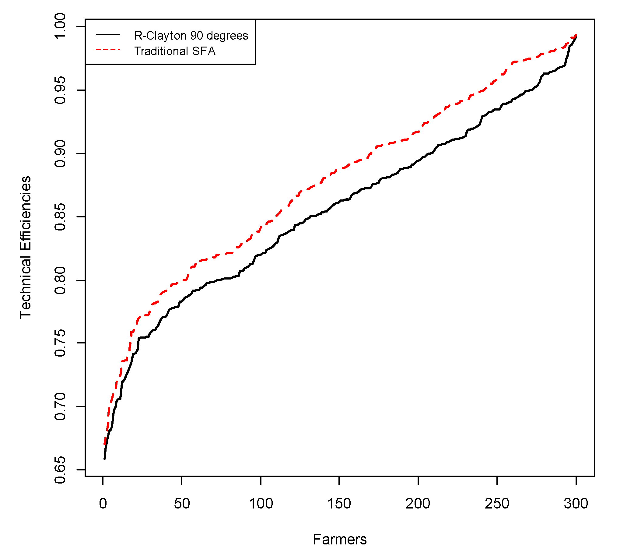
for the conventional SFM with heterogeneity and R-Clayton 90° SFM with dependent error components and heterogeneity. It is clear from Table 4 that the conventional SFM with heterogeneity overestimates technical efficiency levels, and there are differences in the distribution of individual farmers within individual technical efficiency intervals in this case. The mean technical efficiency score from the copula-based model is significantly lower by two points (p < 0.01). In the copula-based SFM with dependent error components and heterogeneity, 29.3% of the farmers are operating at efficiency level of 91% or above, whereas the corresponding figure is 42.3% in the conventional SFM with heterogeneity. Figure 3 presents the cumulative distribution of the technical efficiency scores of the conventional SFM with heterogeneity and copula-based SFM with dependent error components and heterogeneity, which shows large differences as well.

Table 5. Top five and bottom five technical efficiency scores of the individual farmers based on conventional and copula-based SFMs.

Rank	Conventional SFM		R-Clayton 90° SFM
	Farmer ID	TE	Farmer ID	TE
1	38	0.9937	38	0.9924
2	68	0.9916	68	0.9895
3	34	0.9915	34	0.9868
4	69	0.9712	50	0.9853
5	281	0.9878	23	0.9850
…	…	…	…	…
296	135	0.7036	154	0.6819
297	173	0.6985	135	0.6807
298	42	0.6824	178	0.6741
299	185	0.6753	42	0.6668
300	178	0.6702	185	0.6587

presents the shifts in the relative ranks of the top five and bottom five farmers with respect to technical efficiency scores between the conventional SFM with heterogeneity and the copula-based SFM with dependent error components and heterogeneity, thereby, confirming the trends shown in Figure 3. Figure 4 shows the differences of technical efficiency scores between the copula-based SFM with dependent error components and heterogeneity and the conventional SFM with heterogeneity. We can see that the technical efficiency scores are mostly overestimated as compared to the conventional SFM with heterogeneity. Finally,

Table 6. The five maximum and five minimum TE differences between conventional and copula-based SFMs.

Rank	Farmer ID	Technical Efficiency Scores		Differences
		Conventional SFM	R-Clayton 90° SFM
1	250	0.891	0.8433	0.0477
2	251	0.979	0.9332	0.0458
3	248	0.8817	0.8373	0.0443
4	71	0.9372	0.897	0.0402
5	37	0.8998	0.8607	0.0391
…	…	…	…	…
296	23	0.9758	0.9849	−0.0091
297	50	0.9758	0.9853	−0.0094
298	129	0.8167	0.8265	−0.0098
299	128	0.9388	0.9536	−0.0147
300	127	0.8712	0.8872	−0.016

shows that the maximum level of difference in efficiency score is five points and the minimum level of difference is two points between the conventional SFM with heterogeneity and copula-based SFM with dependent error components and heterogeneity, respectively.

4.4. Determinants of Technical Efficiency

The mid-panel of Table 3 presents the results of the inefficiency effects function. Once again, the determinants of technical inefficiency of the copula-based SFM with dependent error components and heterogeneity are different from the traditional SFM with heterogeneity. For example, coefficients on the three of the four socio-economic factors used to explain observed farm specific inefficiency were significantly different from zero at the 1% level at least in the copula-based SFM with dependent error components and heterogeneity, whereas only one variable (i.e., the share of hired labour) was found to be significantly different from zero at the 1% level in the conventional SFM with heterogeneity. Results from the copula-based SFM with dependent error components and heterogeneity reveal that experienced farmers (i.e., older farmers), dependency pressure (larger family size) and the use of hired labour are significantly associated with technical inefficiency, while education has no influence. These results are not unexpected and conform to the literature. For example, Coelli et al. [49] noted that dependency pressure as well as farmers’ experience is negatively associated with technical efficiency in modern rice cultivation in Bangladesh. Similarly, Rahman and Rahman [48] noted that the share of family supplied labour is technically efficient in rice farming in Bangladesh, implying that the use of hired labour is relatively inefficient.

5. Conclusions and Discussion

This study reveals the consequences of assuming independence of error components and ignoring heterogeneity of inefficiency in copula-based SFMs, proposes a copula-based stochastic frontier model with dependent error components and heterogeneity, and empirically applies this to a sample of rice producers from northern Thailand.

The traditional SFM assumes independent error components and does not include heterogeneity (inefficiency effects). Ignoring dependent error components and heterogeneity in the traditional stochastic frontier model lead to the underestimation of model parameters and serious overestimation of technical efficiency. The stochastic frontier model with heterogeneity, namely, the inefficiency frontier model, still assumes independent error components. This assumption also underestimates parameters and produces biased TE scores. In the copula-based stochastic frontier model with dependent error components only (i.e., [14,16]), parameter estimation and TE scores are still biased to some extent due to lack of heterogeneity (inefficiency effects). Therefore, we can conclude that if error components are correlated and heterogeneity exist in the data, the copula-based stochastic frontier with dependent error components and heterogeneity is the best choice. The copula-based stochastic frontier with dependent error components and heterogeneity nests other three models. Therefore, the model proposed in this paper is very flexible.

The empirical case study results also raise the question of reliability of the results obtained from the conventional SFM with heterogeneity. Therefore, for reliable and robust interpretation of results, one may need to test the assumption of independence of the error components, and undertake appropriate measures since violation of this restrictive assumption leads to biased efficiency scores and identification of fewer actual predictors of productivity and efficiency of the firms under investigation, thereby leading to biased and/or misleading conclusions. To sum up, the copula-based models with dependent error components and heterogeneity are more general than the standard SFM model, so we can test validity of the assumption of the independence of the inefficiency component and avoid bias that could arise in the estimated results. The empirical application of our proposed model proves that although the overall underlying production structure of rice farmers are not fundamentally different from what can be discerned from the traditional SFM with independent error components and heterogeneity, our results are more accurate, unbiased and robust with respect to identification of significant production drivers and heterogeneity (i.e., inefficiency effects variables), TE estimates and distribution of TE scores across individual farmers.

Based on our empirical findings, we propose the following policy suggestions for the Thai government and rice farmers. (1) The Thai government should attempt to narrow differences in technical efficiency among rice farmers. This can be achieved by promoting advanced planting technology and technical training to rice farming population. (2) Government should invest in promoting use of agricultural machinery which could replace part of the labor force used in rice farming. Mechanization of agricultural production cannot only improve production efficiency but can also save labor.

Although the proposed model is general and flexible, there are still some questions that need to be explored. One is to investigate the asymmetric effects of independent variables and covariate variables. The asymmetry of datasets may have an impact on estimation. The other area of investigation is to understand how the proposed model effects TFP estimation and its subsequent decomposition into finer components.

References

1. Afriat, S.N. Efficiency estimation of production functions. Int. Econ. Rev. 1972, 13, 568–598. [Google Scholar] [CrossRef]
2. Richmond, J. Estimating the Efficiency of Production. Int. Econ. Rev. 1974, 15, 515–521. [Google Scholar] [CrossRef]
3. Aigner, D.J.; Lovell, C.A.K.; Schmidt, P. Formulation and estimation of Stochastic Frontier Production function models. J. Econom. 1977, 6, 21–37. [Google Scholar] [CrossRef]
4. Meeusen, W.; Broeck, V.D. Efficiency estimation from Cobb-Douglas production function with composed error. Int. Econ. Rev. 1977, 18, 435–455. [Google Scholar] [CrossRef]
5. Greene, W.H. Simulated Likelihood Estimation of the Normal-Gamma Stochastic Frontier Function. J. Product. Anal. 2003, 19, 179–190. [Google Scholar] [CrossRef]
6. Rahman, S.; Wiboonpongse, A.; Sriboonchitta, S.; Chaovanapoonphol, Y. Production efficiency of Jasmine rice farmers in northern and northeastern Thailand. J. Agric. Econ. 2009, 60, 419–435. [Google Scholar] [CrossRef] [Green Version]
7. Obianefo, C.A.; Ng’ombe, J.N.; Mzyece, A.; Masasi, B.; Obiekwe, N.J.; Anumudu, O.O. Technical Efficiency and Technological Gaps of Rice Production in Anambra State, Nigeria. Agriculture 2021, 11, 1240. [Google Scholar] [CrossRef]
8. Anwar, M. Cost efficiency performance of Indonesian banks over the recovery period: A stochastic frontier analysis. Soc. Sci. J. 2019, 56, 377–389. [Google Scholar] [CrossRef]
9. Liu, J.; Wang, M.; Yang, L.; Rahman, S.; Sriboonchitta, S. Agricultural Productivity Growth and Its Determinants in South and Southeast Asian Countries. Sustainability 2020, 12, 4981. [Google Scholar] [CrossRef]
10. Song, F.; Yu, Y. Modelling energy efficiency in China: A fixed-effects panel stochastic frontier approach. Econ. Political Stud. 2018, 6, 158–175. [Google Scholar] [CrossRef]
11. Jiang, W.; Zhang, H.; Lin, Y. Trade Sustainability and Efficiency under the Belt and Road Initiative: A Stochastic Frontier Analysis of China’s Trade Potential at Industry Level. Emerg. Mark. Finance Trade 2022, 58, 1740–1752. [Google Scholar] [CrossRef]
12. Malik, M.A.; Masood, T. A decomposition analysis of total factor productivity growth in MENA countries: Stochastic frontier analysis approach. Middle East Dev. J. 2021, 13, 347–366. [Google Scholar] [CrossRef]
13. Carroll, J.; Newman, C.; Thorne, F. A comparison of stochastic frontier approaches for estimating technical inefficiency and total factor productivity. Appl. Econ. 2011, 43, 4007–4019. [Google Scholar] [CrossRef]
14. Smith, M.D. Stochastic frontier models with dependent error components. Econom. J. 2008, 11, 172–192. [Google Scholar] [CrossRef]
15. Mehdi, R.E.; Hafner, C.M. Inference in stochastic frontier analysis with dependent error terms. Math. Comput. Simul. 2014, 102, 131–143. [Google Scholar] [CrossRef]
16. Wiboonpongse, A.; Liu, J.; Sriboonchitta, S.; Denoeux, T. Modelling dependence between error components of the stochastic frontier model using copula: Application to intercrop coffee production in northern Thailand. Int. J. Approx. Reason. 2015, 65, 34–44. [Google Scholar] [CrossRef]
17. Bonanno, G.; De Giovanni, D.; Domma, F. The “wrong skewness” problem: A re-specification of stochastic frontiers. J. Prod. Anal. 2017, 47, 49–64. [Google Scholar] [CrossRef] [Green Version]
18. Amsler, C.; Prokhorov, A.; Schmidt, P. Using Copulas to Model Time Dependence in Stochastic Frontier Models. Econom. Rev. 2014, 33, 497–522. [Google Scholar] [CrossRef]
19. Lai, H.; Kumbhakar, S.C. Panel Stochastic Frontier Model with Endogenous Inputs and Correlated Random Components. J. Bus. Econ. Stat. 2021, 2021, 1–17. [Google Scholar]
20. Wei, Z.; Conlon, E.M.; Wang, T. Asymmetric dependence in the stochastic frontier model using skew normal copula. Int. J. Approx. Reason. 2021, 128, 56–68. [Google Scholar] [CrossRef]
21. Sriboonchitta, S.; Liu, J.; Wiboonpongse, A.; Denoeux, T. A double-copula stochastic frontier model with dependent error components and correction for sample selection. Int. J. Approx. Reason. 2017, 80, 174–184. [Google Scholar] [CrossRef] [Green Version]
22. Battese, G.; Coelli, T. A model for technical inefficiency effects in a stochastic frontier production function for panel data. Empir. Econ. 1995, 20, 325–332. [Google Scholar] [CrossRef] [Green Version]
23. Carta, A.; Steel, M.F. Modelling multi-output stochastic frontiers using copulas. Comput. Stat. Data Anal. 2012, 56, 3757–3773. [Google Scholar] [CrossRef] [Green Version]
24. Yuan, X.; Tang, J.; Wong, W.-K.; Sriboonchitta, S. Modeling Co-Movement among Different Agricultural Commodity Markets: A Copula-GARCH Approach. Sustainability 2020, 12, 393. [Google Scholar] [CrossRef] [Green Version]
25. Huang, T.-H.; Hu, C.-N.; Chang, B.-G. Competition, efficiency, and innovation in Taiwan’s banking industry—An application of copula methods. Q. Rev. Econ. Financ. 2018, 67, 362–375. [Google Scholar] [CrossRef]
26. Maria, E.C.J.; Salazar, I.; Sanz, L.; Villegas, M.A.G. Using Copula to Model Dependence When Testing Multiple Hypotheses in DNA Microarray Experiments: A Bayesian Approximation. Mathematics 2020, 8, 1514. [Google Scholar] [CrossRef]
27. Yamaka, W.; Maneejuk, P. Analyzing the Causality and Dependence between Gold Shocks and Asian Emerging Stock Markets: A Smooth Transition Copula Approach. Mathematic 2020, 8, 120. [Google Scholar] [CrossRef] [Green Version]
28. Wei, Z.; Kim, S.; Choi, B.; Kim, D. Multivariate Skew Normal Copula for Asymmetric Dependence: Estimation and Application. Int. J. Inf. Technol. Decis. Mak. 2019, 18, 365–387. [Google Scholar] [CrossRef]
29. Sklar, S. Fonctions de repartition ‘an dimensions et leurs marges. Publ. Inst. Statist. Univ. Paris 1959, 8, 229–231. [Google Scholar]
30. Boyer, B.H.; Gibson, M.S.; Loretan, M. Pitfalls in Tests for Changes in Correlations; IFS Discussion Paper No 597R; Federal Reserves Board: Washington, DC, USA, 1999.
31. Schmidt, R. Tail dependence for elliptically contoured distributions. Math. Methods OR 2002, 55, 301–327. [Google Scholar] [CrossRef]
32. Brechmann, E.C.; Schepsmeier, U. Modelling Dependence with C- and D-Vine Copulas: The R Package CDVine. J. Stat. Softw. 2013, 52, 1–29. [Google Scholar] [CrossRef] [Green Version]
33. Sriboonchitta, S.; Nguyen, H.T.; Wiboonpongse, A.; Liu, J. Modelling volatility and dependency of agricultural price and production indices of Thailand: Static versus time-varying copulas. Int. J. Approx. Reason. 2013, 54, 793–808. [Google Scholar] [CrossRef]
34. Cech, C. Copula-Based Top-Down Approaches in Financial Risk Aggregation; University of Applied Sciences BFI Vienna: Vienna, Austria, 2006. [Google Scholar]
35. Luo, J. Stepwise Estimation of D-Vines with Arbitrary Specified Copula Pairs and EDA Tools. Ph.D. Thesis, Technische Universitaet Muenchen, Munich, Germany, 2010. [Google Scholar]
36. Coelli, T.J. Estimators and hypothesis tests for a stochastic frontier function: A Monte-Carlo analysis. J. Product. Anal. 1995, 6, 247–268. [Google Scholar] [CrossRef]
37. Guo, X.; Li, G.-R.; McAleer, M.; Wong, W.-K. Specification Testing of Production in a Stochastic Frontier Model. Sustainability 2018, 10, 3082. [Google Scholar] [CrossRef] [Green Version]
38. Wang, H.-J.; Schmidt, P. One-step and two-step estimation of the effects of exogenous variables on technical efficiency levels. J. Product. Anal. 2002, 18, 129–144. [Google Scholar] [CrossRef]
39. Burns, R. The Simulated Maximum Likelihood Estimation of Stochastic Frontier Models with Correlated Error Components; The University of Sydney: Camperdown, NSW, Australia, 2004. [Google Scholar]
40. Liu, J.; Songsak, S.; Aree, W.; Thierry, D. A trivariate Gaussian copula stochastic frontier model with sample selection. Int. J. Approx. Reason. 2021, 137, 181–198. [Google Scholar] [CrossRef]
41. Greene, W.H. Distinguishing between heterogeneity and inefficiency: Stochastic Frontier Analysis of the World Health Organization’s Panel Data on National Health Care Systems. Health Econ. 2004, 13, 959–980. [Google Scholar] [CrossRef]
42. Lai, H.-P.; Huang, C.J. Maximum likelihood estimation of seemingly unrelated stochastic frontier regressions. J. Product. Anal. 2013, 40, 1–14. [Google Scholar] [CrossRef]
43. Joe, H. Multivariate Models and Dependence Concepts; Chapman and Hall: London, UK, 1997. [Google Scholar]
44. Wei, Z.; Zhu, X.; Wang, T. The extended skew-normal-based stochastic frontier model with a solution to “wrong skewness” problem. Statistics 2021, 55, 1387–1406. [Google Scholar] [CrossRef]
45. Liu, J.; Wang, M.; Ma, J.; Rahman, S.; Sriboonchitta, S. A Simultaneous Stochastic Frontier Model with Dependent Error Components and Dependent Composite Errors: An Application to Chinese Banking Industry. Mathematics 2020, 8, 238. [Google Scholar] [CrossRef] [Green Version]
46. Zhu, X.; Zheng, W.; Wang, T. Multivariate Skew Normal-Based Stochastic Frontier Models. J. Stat. Theory Pract. 2022, 16, 20. [Google Scholar] [CrossRef]
47. Rahman, S.; Hasan, M.K. Impact of environmental production conditions on productivity and efficiency: The case of wheat producers in Bangladesh. J. Environ. Manag. 2008, 88, 1495–1504. [Google Scholar] [CrossRef] [PubMed] [Green Version]
48. Rahman, S.; Rahman, M. Impact of land fragmentation and resource ownership on productivity and efficiency: The case of rice producers in Bangladesh. Land Use Policy 2009, 26, 95–103. [Google Scholar] [CrossRef] [Green Version]
49. Coelli, T.; Rahman, S.; Thirtle, C. Technical, allocative, cost and scale efficiencies in Bangladesh rice cultivation: A non-parametric approach. J. Agric. Econ. 2002, 53, 607–626. [Google Scholar] [CrossRef]
Figure 1. Histograms of TE for Models 1–6 and True parameters.
Agriculture 12 01078 g001
Figure 2. Histogram of the differences of TE scores. The differences mean that the estimated TE scores of Model 6 subtract true TE for the opposite simulation.
Agriculture 12 01078 g002
Figure 3. Cumulative technical efficiency distribution of conventional SFM and copula-based SFM.
Agriculture 12 01078 g003
Figure 4. Differences in absolute individual efficiency estimates.
Agriculture 12 01078 g004