The Impacts of Climate Change on Water Resources and Crop Production in an Arid Region

Abstract

Climate change is one of the most pressing global issues of the twenty-first century. This phenomenon has an increasingly severe impact on water resources and crop production. The main purpose of this study is to evaluate the impact of climate change on water resources, crop production, and agricultural sustainability in an arid environment in Iran. To this end, the study constructs a new integrated climate-hydrological-economic model to assess the impact of future climate change on water resources and crop production. Furthermore, the agricultural sustainability is evaluated using the multicriteria decision making (MCDM) technique in the context of climate change. The findings regarding the prediction of climate variables show that the minimum and maximum temperatures are expected to increase by about 5.88% and 6.05%, respectively, while precipitation would decrease by approximately 30.68%. The results of the research reveal that water availability will decrease by about 13.79–15.45% under different climate scenarios. Additionally, the findings show that in the majority of cases crop production will reduce in response to climate scenarios so that rainfed wheat will experience the greatest decline (approximately 59.95%). The results of the MCDM model show that climate change can have adverse effects on economic and environmental aspects and, consequently, on the sustainability of the agricultural system of the study area. Our findings can inform policymakers on effective strategies for mitigating the consequences of climate change on water resources and agricultural production in dry regions.

1. Introduction

Climate change’s impact on agricultural production has raised serious global concerns in the twenty-first century [1,2]. Carbon dioxide (CO₂) emissions have been identified as the primary cause of climate change [3,4,5]. Human activities, such as the use of fossil fuels, environmental degradation, and land-use changes, have all contributed significantly to rising CO₂ levels in the atmosphere since the industrial revolution [6,7,8,9]. The global CO₂ concentration in the atmosphere increased from 288 ppm in 1750 to 415 ppm in 2021 [10]. This has resulted in higher global average temperatures and unpredictability of rainfall patterns [11]. Climate change and variability have far-reaching consequences for natural resources, human communities, and biodiversity [12]. Water resources and agriculture are most affected by climate change because it directly determines the availability of resources in terms of time and space [13]. Some researchers have concluded that climate change has a negative impact on groundwater table recharge, which affects irrigation [12,14]. Others believe that this phenomenon will increase agricultural water demand due to increased evapotranspiration, thus putting more pressure on water resources [12,15]. Aside from influencing the availability of water resources, climate change is expected to reduce crop yield and agricultural efficiency by increasing crop water stress [16]. Climate change has recently had a negative impact on crop production in major agricultural areas; it is also expected to reduce global agricultural production by about 16% by 2030, resulting in widespread food insecurity [17,18,19]. Therefore, meeting the food needs of the world’s rising population has become a major concern around the world [2,20].

Climate change is expected to have the greatest impact on agricultural production in the world’s dry and semi-arid regions, such as Iran. Iran’s average annual rainfall is around 250 mm, which is less than one-third of the global average; therefore, most parts of the country suffer from a lack of water resources for food production [21]. Nevertheless, the adaptation of supportive polices to achieve self-sufficiency in order to meet the domestic food demand in the presence of climate change has led to increased pressure on water resources in the country’s arid and semi-arid regions [22,23]. In this regard, the Mashhad plain in northeastern Iran serves as a good example. Climate data analysis reveals that the phenomenon of climate change has happened in this area as a result of decreasing rainfall and increasing temperature (see Figure 1). As shown in the figure, during the years 1990 to 2016, the total precipitation decreased from 300 mm to 220 mm and the average temperature increased from 11.9 °C to 16.5 °C. Given the importance of this plain in ensuring the country’s food security, a thorough understanding of the effects of climate change on water resources and agricultural production in this region is required to adopt accurate and efficient mitigation and adaptation policies.

The literature review indicated that the effects of climate change on water resources and crop production have been studied all over the world. Xiong et al. [24] used climate scenarios of the regional climate model to investigate the consequences of climate change on water availability and cereal production in China in the 2020s and 2040s. The findings of this study revealed that there are insufficient water resources for cereal production, particularly in southern China, due to an increase in nonagricultural water demand and the occurrence of climate change. Palazzoli et al. [16] developed a soil and water assessment tool (SWAT) model to investigate the effects of future climate change on rainfed crop productivity and water resources in Nepal. Based on their results, they predicted significant potential changes in water resources availability (from −26 to +37%) and crop production (rice from −17 to +12%, wheat from −36 to +18% and maize from −17 to +4%). Sinnarong et al. [25] applied an econometric model to estimate the effect of climate change on rice production in Thailand. The results showed that temperature has a negative impact on rice production while precipitation has different regional effects on rice production. Additionally, the findings indicated that rice production under different climatic scenarios would decrease between 4.56% and 33.77%. Mostafa et al. [26] evaluated the impact of climate change on water resources and the agricultural sector of Egypt using climate and irrigation (CROPWAT) models and found the irrigation water requirement for wheat crop would rise by about 6.2% in 2050 and 11.8% in 2100. Furthermore, wheat production would decrease by approximately 8.6% and 11.1% in 2050 and 2100, respectively. Medellín-Azuara et al. [27] estimated the impact of climatic change on crop farming in California using the statewide agricultural production model (SWAP). They found that, by 2050, water supply, agricultural land use, and production of most crops will decrease in California due to climate change, such as rising temperature and declining precipitation. Shahvari et al. [28], using the SWAT model, assessed the impact of climate change on water resources and crop yield in Iran for the future. Their results revealed that future climate scenarios will lead to an increase in runoff in spring and autumn and a decrease in summer and winter. In addition, future climate change will reduce the yield of rainfed crops in the region. Lu et al. [29] constructed a new climate-economic model to analyze the effects of climate change on grain production and water resources. The findings of this study showed that irrigation water consumption has increased by about 100 billion m³ because of climate change in China. This phenomenon also reduced the grain yield in this area by 1000 kg/hm². The current gap in the existing literature is a comprehensive view of all meteorological, hydrological, economic, and sustainability aspects of climate change in the agricultural sector.

The study, therefore, assesses the effect of future climate change on water resources, crop production, and agricultural sustainability in the Mashhad plain under three climate scenarios (RCP 2.6, 4.5, and 8.5). Specifically, the study aims at (1) projecting climate variables using the Long Ashton Research Station Weather Generator (LARS-WG) model alongside HadGEM2-ES outputs and the three RCP scenarios; (2) assessing the impact of future climate change on water resources in the Mashhad plain using panel data model; (3) estimating the relationship between crop yield and climate variables, including minimum temperature, maximum temperature, and precipitation, using the GME (generalized maximum entropy) technique; (4) investigating the impact of climate change on cropping pattern, crop production, and water consumption in the selected area using PMP (positive mathematical programming) model; (5) evaluating the agricultural sustainability under climate scenarios using a MCDM (multicriteria decision making) method. The results of this study are expected to provide policymakers with insights into designing climate change mitigation policies to ensure food security and sustainable production in the region.

The contribution of this study to the literature is twofold. First, to the best of our knowledge, this is the first attempt to apply an integrated climate-hydrological-economic model to evaluate the effect of climate change on water resources, crop production, and cropping pattern in Iran. The second contribution of the study is found in the use of the MCDM approach to investigate the sustainability of agricultural activity at the regional level under different climate scenarios.

The study is structured as follows: Section 2 describes the study area, datasets, and methodology. Section 3 presents the results and discussions, and the last section concludes with the research and policy implications of these findings.

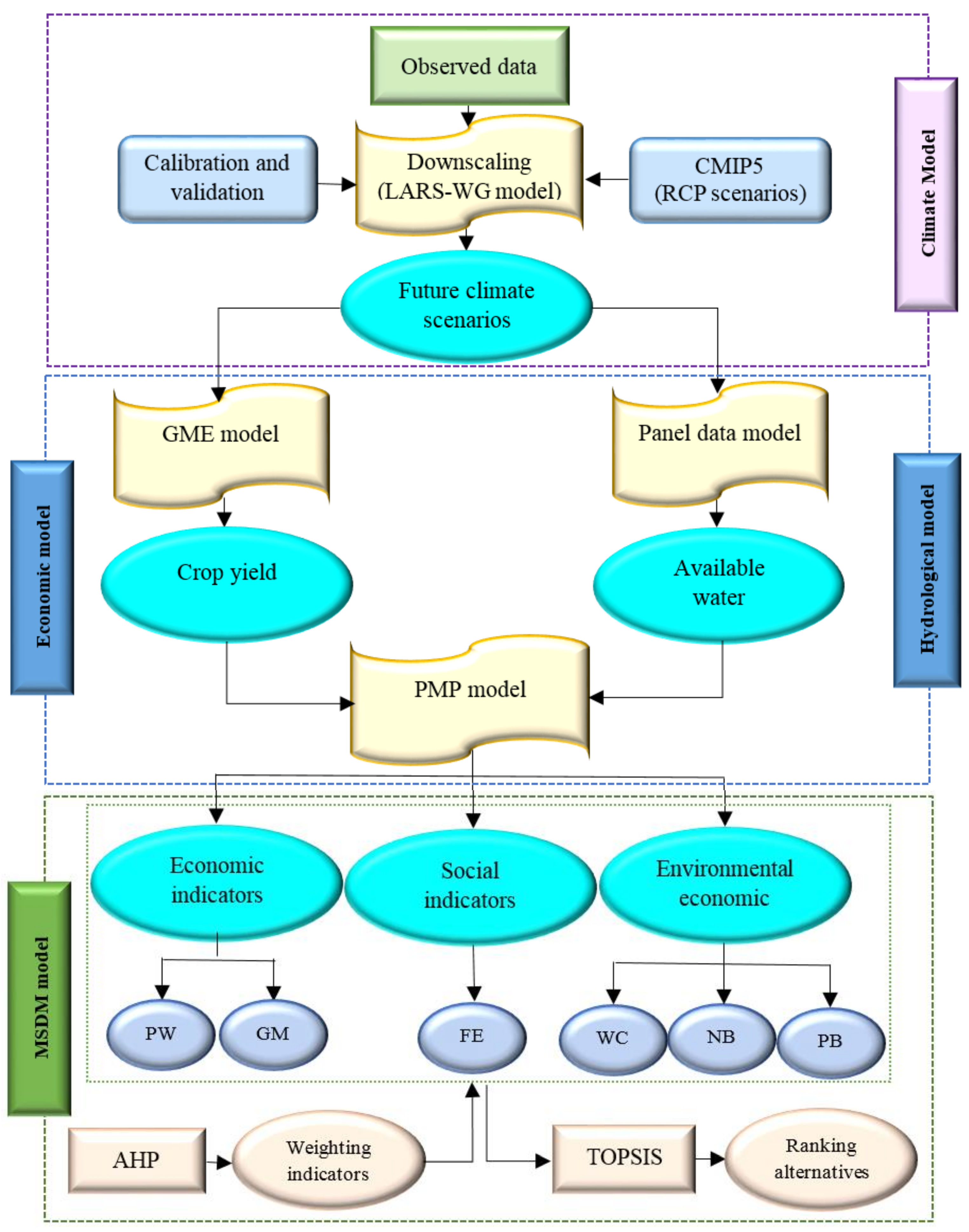
2. Materials and Methods

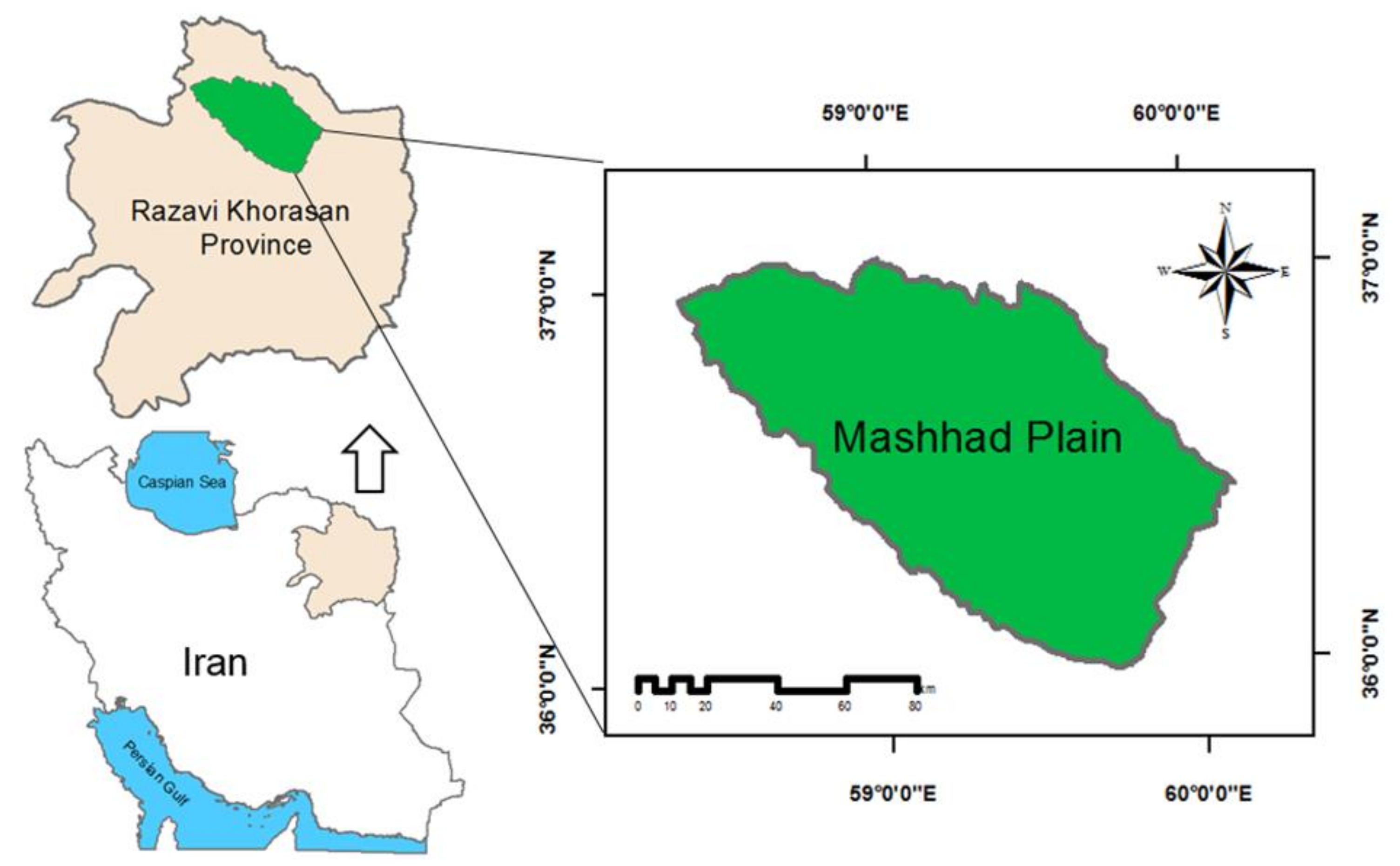
This study used a variety of methods to achieve its research goals. The LARS-WG model was used to downscale the climate variables (maximum and minimum temperatures and precipitation), and a regression model was used to forecast the groundwater availability in the Mashhad plain. The sensitivity of yield to climate change was estimated using the GME technique. The cropping pattern was then evaluated under climate change using a PMP model. Finally, economic, social, and environmental indicators were ranked using an integrated MCDM method. The complete structure of the framework is presented in Figure 2.

2.1. Study Area

The present case study is in Northeast Khorasan Razavi Province, Iran, between the latitude 35°59′ to 37°03′ N and longitude 58°22′ to 60°06′ E, covering an area of approximately 9957 km². The plain is bounded on the north by Hezar Masjid heights, on the northwest by Atrak river basin, on the south by Binaloud Mountain, and on the southeast by Jamroud river basin [30]. It has a semi-arid to arid climate, with an average annual rainfall from 1991 to 2015 is about 262 mm [31]. The average monthly temperature in this plain is reported to be between 11.6 °C and 26.7 °C. Furthermore, the average annual evapotranspiration ranges from 236 to 310 (mm). The location of the study area is shown in Figure 3. Around 3 million people live in the study basin and rely mostly on groundwater resources for drinking and agricultural cultivation. Climate change and a lack of water resource management in this area have resulted in a 12-m water drop in the water table over a 20-year period [32].

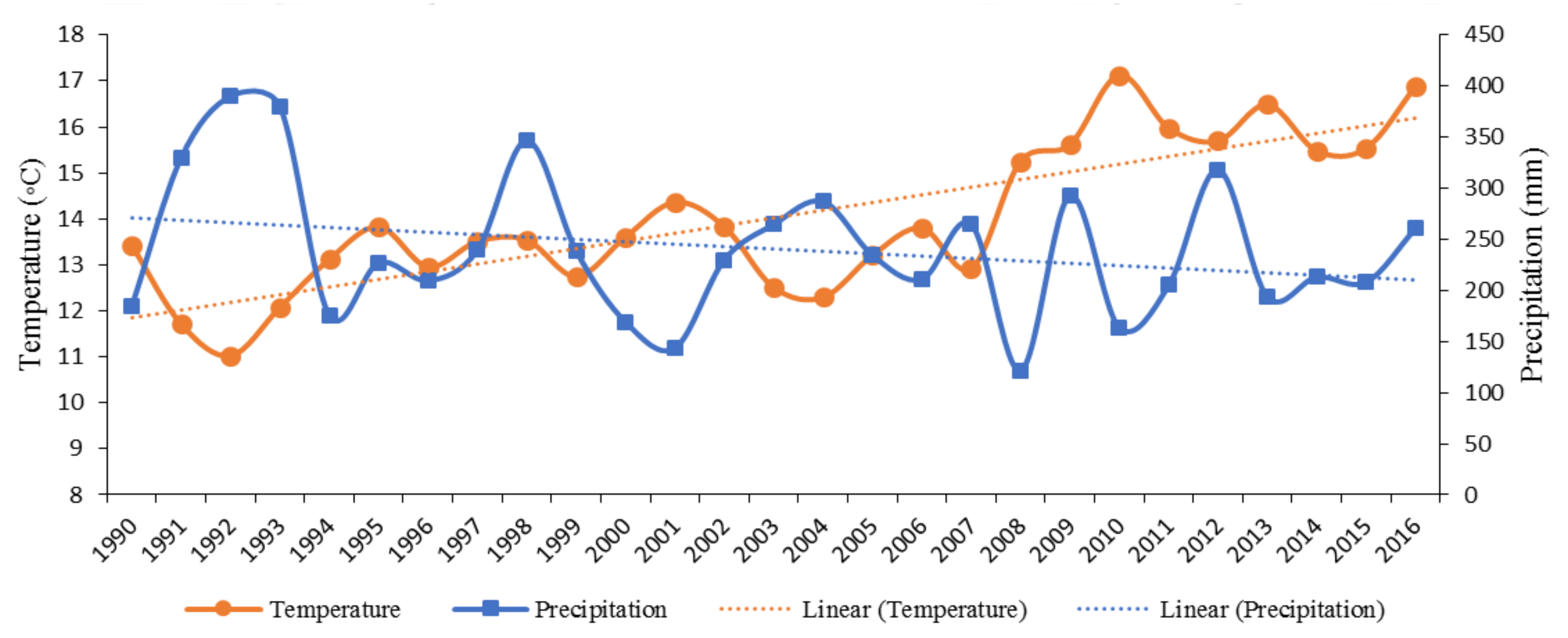
2.2. Data Collection

The observed daily time series data of minimum temperature, maximum temperature, and precipitation for Mashhad synoptic station during the period 1979–2016 were obtained from Iran’s Meteorological Organization. To estimate the model (Equation (6)), the data (2000–2016) on piezometric wells and groundwater depth in the Mashhad plain were provided by Iran Water Resources Management Company. Additionally, the observed monthly temperature and precipitation data (2000–2016) for the synoptic station were obtained from Iran’s Meteorological Organization. To estimate the yield response function (Equation (8)), crop yield data (1983–2016) were gathered from Ministry of Agriculture Jihad of Iran. Figure 4 shows the growing seasons of crops (wheat, barley, alfalfa, potato, corn, tomato, melon, onion, sugar beet, and cucumber) in the Mashhad plain. Data and information on outputs prices, inputs costs, technical coefficients, crop yield, and resources availability were gathered through face-to-face interviews with farmers in 2016–2017 cropping season.

2.3. Meteorological Model

The LARS-WG model is a random generator that uses statistical downscaling techniques to generate meteorological data [33]. Because of the repeated calculations, it requires less input data and is simpler and more efficient than other models [34,35]. Racsko et al. [36] proposed this model, which Semenov et al. [37] later revised and developed. This model’s sixth version (LARS-WG6) was updated in 2018 for downscaling the coupled model intercomparison project phase (CIMP5) [34]. The HadGEM2-ES universal model data were used in this study to project climate variables during the horizon in 2045 under three climate scenarios, namely RCP 2.6, RCP 4.5, and RCP 8.5. The LARS-WG model was implemented using daily data of maximum and minimum temperature and precipitation from 1979 to 2016.

The performance of the LARS-WG statistical model was evaluated by comparing the simulated and observed maximum and minimum temperatures, as well as precipitation, using the following statistics [2,38,39]: coefficient of determination (R²), normalized root mean square error (NRMSE), root mean square error (RMSE), mean absolute deviation (MAD), and mean square error (MSE) (see

Table 1. The statistical indicators for model validation.

Index	Formulate	Model Performance
${\mathrm{R}}^2$	${\mathrm{R}}^2=\frac{({{\displaystyle \sum }}_{\mathrm{n}=1}^{\mathrm{N}}({\mathrm{S}}_{\mathrm{n}}-\overline{\mathrm{S}})({\mathrm{O}}_{\mathrm{n}}-\overline{\mathrm{O}}){)}^2}{{{\displaystyle \sum }}_{\mathrm{n}=1}^{\mathrm{N}}{({\mathrm{S}}_{\mathrm{n}}-\overline{\mathrm{S}})}^2{{\displaystyle \sum }}_{\mathrm{n}=1}^{\mathrm{N}}{({\mathrm{O}}_{\mathrm{n}}-\overline{\mathrm{O}})}^2}$	≤0.75
$\mathrm{NRMSE}$	$\mathrm{NRMSE}=\frac{\mathrm{RMSE}}{\overline{\mathrm{O}}}\times 100$	Criteria ≤10% 10–20% 20–30% ≥30%	performance Excellent Good Fair Poor
$\mathrm{RMSE}$	$\mathrm{RMSE}=\sqrt{\frac{{{\displaystyle \sum }}_{\mathrm{n}=1}^{\mathrm{N}}{({\mathrm{S}}_{\mathrm{n}}-{\mathrm{O}}_{\mathrm{n}})}^2}{\mathrm{N}}}$	the lower values show a better model [40]
$\mathrm{MAD}$	$\mathrm{MAD}=\frac{{{\displaystyle \sum }}_{\mathrm{n}=1}^{\mathrm{N}}\left|{\mathrm{S}}_{\mathrm{n}}-{\mathrm{O}}_{\mathrm{n}}\right|}{\mathrm{N}}$
$\mathrm{MSE}$	$\mathrm{MSE}=\frac{{{\displaystyle \sum }}_{\mathrm{n}=1}^{\mathrm{N}}{\left({\mathrm{S}}_{\mathrm{n}}-{\mathrm{O}}_{\mathrm{n}}\right)}^2}{\mathrm{N}}$

Note: N is the number of data points, ${\mathrm{S}}_{\mathrm{n}}$is the simulated values, ${\mathrm{O}}_{\mathrm{n}}$ is the observed values, $\overline{\mathrm{O}}$ is the mean of the observed values, and $\overline{\mathrm{S}}$ is the mean of the simulated values.

).

2.4. Hydrological Model

This section investigates the effects of climate change on groundwater resources in the Mashhad plain. The panel data model was used to forecast the groundwater depth in the plain. To this end, the following groundwater conceptual model was estimated using panel data regression [41,42] related to piezometers as cross units from 2000 to 2016.

$${\mathrm{lnH}}_{\mathrm{t}}={\mathsf{\alpha }}_0+{\mathsf{\alpha }}_1{\mathrm{lnH}}_{\mathrm{t}-1}+{\mathsf{\alpha }}_2{\mathrm{lnP}}_{\mathrm{t}-1}+{\mathsf{\alpha }}_3{\mathrm{lnTmin}}_{\mathrm{t}-1}+{\mathsf{\alpha }}_4{\mathrm{lnTmax}}_{\mathrm{t}-1}$$

(1)

where t indicates time, ${\mathrm{H}}_{\mathrm{t}}$ is predicted groundwater depth, ${\mathrm{H}}_{\mathrm{t}-1}$is the initial groundwater depth, P is total monthly precipitation (mm), Tmin and Tmax are monthly minimum and maximum temperature (°C), respectively, and ${\mathsf{\alpha }}_0$ to ${\mathsf{\alpha }}_4$ are the model coefficients that should be estimated.

After estimating the amount of changes in groundwater depth because of climate change, Equation (2) was used to calculate the amount of changes in groundwater resources [43,44,45,46].

$$\Delta \mathrm{V}=\mathrm{A}\times {\mathrm{S}}_{\mathrm{y}}\times \Delta \mathrm{H}$$

(2)

where $\Delta \mathrm{V}$ is the groundwater storage change (m³), $\mathrm{A}$ is geographical area (m²), ${\mathrm{S}}_{\mathrm{y}}$ is specific yield (dimensionless), and $\Delta \mathrm{H}$ is average depth change (m).

2.5. Economic Models

2.5.1. Generalized Maximum Entropy (GME) Model

In this study, the Cobb–Douglas Yield Response (CDYR) model was used to assess the sensitivity of crops yield to climatic variables, such as minimum and maximum temperatures, as well as precipitation [47,48]. The CDYR model, after taking the logarithm of both sides of the equation, can be presented as follows:

$$\log ({\mathrm{Y}}_{\mathrm{t}})={\mathsf{\beta }}_0 +{\mathsf{\alpha }}_{\mathrm{t}}\log ({\mathrm{Tmin}}_{\mathrm{t}})+{\mathsf{\lambda }}_{\mathrm{t}}\log ({\mathrm{Tmax}}_{\mathrm{t}})+{\mathsf{\eta }}_{\mathrm{t}}\log \left({\mathrm{P}}_{\mathrm{t}}\right)+\mathsf{\nu }\mathrm{Trend}$$

(3)

where t is the set of years; Y is the yield of crops (wheat, barley, alfalfa, potato, corn, tomato, melon, onion, sugar beet, and cucumber); $\mathrm{Tmin}$ and $\mathrm{Tmax}$ are average minimum and maximum temperature; and $\mathrm{P}$ is total growing season precipitation. It is worth noting that the impact of additional factors affecting crop production, which were not incorporated in Equation (3), was covered in the residual terms [49].

Due to the lack of access to crop yields data in the research area, we only analyzed data of 34 years (1983–2016). In this case, because of the limited sample size, traditional estimation approaches, such as ordinary least squares (OLS), may result in parameter estimation with excessive variance [49,50]. To address this issue, following Moreno et al. [51], we used the GME estimator. The GME approaches are founded on Shannon’s entropy information measure and the generalized maximum entropy theory [50,52]. Instead of calculating the mean and variance of coefficients directly, GME estimator considers a probability distribution for the coefficients and error terms [52]. Assume that y is dependent on K independent variables ${\mathrm{x}}_{\mathrm{k}}\left(\mathrm{k}=1,\dots ,\mathrm{k}\right)$:

$$\mathrm{y}=\mathrm{X}\mathsf{\beta }+\mathsf{\epsilon }$$

(4)

where y is a (T × 1) vector of observations for y, X is a $\left(\mathrm{T}\times \mathrm{K}\right)$matrix of observations for the ${\mathrm{x}}_{\mathrm{k}}$ variables, $\mathsf{\beta }$ is the $\left(\mathrm{K}\times 1\right)$vector of explanatory variable coefficients, and$\mathsf{\epsilon }$ is a (T × 1) vector of residual terms. To estimate explanatory variable coefficients using GME, firstly we reparametrize the regression model, and then we recast the coefficients and residual in terms of discrete probability distributions.

In this method, each ${\mathsf{\beta }}_{\mathrm{k}}$ is assumed to be as a discrete point with M dimension $\left(\mathrm{M}\ge 2\right)$. Let ${\mathrm{Z}}_{\mathrm{k}}=\left[{\mathrm{Z}}_{\mathrm{k}1},\dots ,{\mathrm{Z}}_{\mathrm{kM}}\right]$ be support points for parameter ${\mathsf{\beta }}_{\mathrm{k}}$, which are symmetrical around zero. Additionally, the probability mass function of ${\mathrm{z}}_{\mathrm{k}}$ is defined as ${\mathrm{P}}_{\mathrm{k}}={\left[{\mathrm{P}}_{\mathrm{k}1},\dots ,{\mathrm{P}}_{\mathrm{kM}}\right]}^{\prime }$ such that:

$${\mathsf{\beta }}_{\mathrm{k}}={\mathrm{E}}_{\mathrm{pk}}\left[{\mathrm{z}}_{\mathrm{k}}\right]={\acute{\mathrm{z}}}_{\mathrm{k}}{\mathrm{p}}_{\mathrm{k}}={\displaystyle \sum }_{\mathrm{m}=1}^{\mathrm{M}}{\mathrm{z}}_{\mathrm{km}}{\mathrm{p}}_{\mathrm{km}};\forall \mathrm{K}=1,\dots ,\mathrm{K}$$

(5)

Then, $\mathsf{\beta }$ can be represented as follows:

$$\mathsf{{\rm B}}=\left[\begin{array}{c}{\mathsf{\beta }}_1\\ ⋮\\ {\mathsf{\beta }}_{\mathrm{K}}\end{array}\right]={\mathrm{z}}_{\mathrm{P}}=\left[\begin{array}{ccc}\begin{array}{c}{\acute{\mathrm{z}}}_1\\ 0\end{array}& \begin{array}{c}0\\ {\acute{\mathrm{z}}}_2\end{array}& \begin{array}{c}\begin{array}{cc}\dots & 0\end{array}\\ \begin{array}{cc}\dots & 0\end{array}\end{array}\\ ⋮& ⋮& \begin{array}{cc}\ddots & ⋮\end{array}\\ 0& 0& \begin{array}{cc}\dots & {\acute{\mathrm{z}}}_{\mathrm{K}}\end{array}\end{array}\right]\left[\begin{array}{c}\begin{array}{c}{\mathrm{P}}_1\\ {\mathrm{P}}_2\end{array}\\ ⋮\\ {\mathrm{P}}_{\mathrm{K}}\end{array}\right]$$

(6)

where Z is a (K × KM) matrix of support values, and P is a (KM × 1) of vector of unknown weights.

The unknown error is defined as follows:

$${\mathsf{\epsilon }}_{\mathrm{g}}={\mathrm{E}}_{{\mathrm{w}}_{\mathrm{g}}}\left[\mathrm{v}\right]=\acute{\mathrm{v}}{\mathrm{w}}_{\mathrm{g}}={\displaystyle \sum }_{\mathrm{j}=1}^{\mathrm{J}}{\mathrm{v}}_{\mathrm{j}}{\mathrm{w}}_{\mathrm{gj}};\forall \mathrm{g}=1,\dots ,\mathrm{G}$$

(7)

where ${\mathrm{w}}_{\mathrm{g}}={\left[{\mathrm{w}}_{\mathrm{g}1},\dots ,{\mathrm{w}}_{\mathrm{gJ}}\right]}^{\prime }$ is a vector of weights, and $\acute{{\mathrm{v}}_{\mathrm{g}}}=\left[{\mathrm{v}}_{\mathrm{g}1},\dots ,{\mathrm{v}}_{\mathrm{gJ}}\right]\left(\mathrm{J}\ge 2\right)$is a set of support points. The error vector is presented as follows:

$$\mathsf{\epsilon }=\left[\begin{array}{c}{\mathsf{\epsilon }}_1\\ ⋮\\ {\mathsf{\epsilon }}_{\mathrm{G}}\end{array}\right]={\mathrm{V}}_{\mathrm{w}}=\left[\begin{array}{ccc}\begin{array}{c}\acute{{\mathrm{v}}_1}\\ 0\end{array}& \begin{array}{c}0\\ \acute{{\mathrm{v}}_2}\end{array}& \begin{array}{cc}\begin{array}{c}\dots \\ \dots \end{array}& \begin{array}{c}0\\ 0\end{array}\end{array}\\ ⋮& ⋮& \begin{array}{cc}\ddots & ⋮\end{array}\\ 0& 0& \begin{array}{cc}\dots & \acute{{\mathrm{v}}_{\mathrm{G}}}\end{array}\end{array}\right]\left[\begin{array}{c}\begin{array}{c}{\mathrm{w}}_1\\ {\mathrm{w}}_2\end{array}\\ ⋮\\ {\mathrm{w}}_{\mathrm{G}}\end{array}\right]$$

(8)

Now, Equation (9) can be extended as follows:

$$\mathrm{y}=\mathrm{XZp}+\mathrm{Vw}$$

(9)

In Equation (9), y, Z, and V are known vectors, and P and w are unknown vectors that are estimated using GME, which is defined as follows:

$$\mathrm{Max}\mathrm{H}\left(\mathrm{p},\mathrm{w}\right)=-{\displaystyle \sum }_{\mathrm{k}=1}^{\mathrm{K}}{\displaystyle \sum }_{\mathrm{m}=1}^{\mathrm{M}}{\mathrm{p}}_{\mathrm{km}}\ln \left({\mathrm{p}}_{\mathrm{km}}\right)-{\displaystyle \sum }_{\mathrm{g}=1}^{\mathrm{G}}{\displaystyle \sum }_{\mathrm{j}=1}^{\mathrm{J}}{\mathrm{w}}_{\mathrm{gj}}\ln \left({\mathrm{w}}_{\mathrm{gj}}\right)$$

(10)

and is subject to:

$${\displaystyle \sum }_{\mathrm{k}=1}^{\mathrm{K}}{\displaystyle \sum }_{\mathrm{m}=1}^{\mathrm{M}}{\mathrm{Z}}_{\mathrm{km}}{\mathrm{P}}_{\mathrm{km}}+{\displaystyle \sum }_{\mathrm{j}=1}^{\mathrm{J}}{\mathrm{v}}_{\mathrm{j}}{\mathrm{w}}_{\mathrm{gj}}={\mathrm{y}}_{\mathrm{g}};\forall \mathrm{g}=1,\dots ,\mathrm{G}$$

(11)

$${\displaystyle \sum }_{\mathrm{k}=1}^{\mathrm{K}}{\mathrm{p}}_{\mathrm{km}}=1;\forall \mathrm{m}=1,\dots ,\mathrm{M}$$

(12)

$${\displaystyle \sum }_{\mathrm{j}=1}^{\mathrm{J}}{\mathrm{w}}_{\mathrm{gj}}=1;\forall \mathrm{g}=1,\dots ,\mathrm{G}$$

(13)

The GME techniques are created by solving the optimization problem (Equation (10)) while taking constraint into account (Equations (11–13)). Equation (11) is a condition for the compatibility of the probability of the posterior distribution of the coefficients and the residual terms with the observations. Equations (12) and (13) are normalization constraints for the probabilities.

2.5.2. Positive Mathematical Programming (PMP) Model

The present study used an economic modeling system composed of the PMP model to analyze and assess the effects of climate change (the decline in available water and the changes in crop yields) on the cropping pattern of selected crops and farmers’ gross revenues in Mashhad plain.

In recent decades, PMP has been widely used to evaluate the effects of climate change on the agricultural sectors [53,54,55,56,57,58]. The main objective of the PMP is to improve the accuracy of modeling farmers’ behavior in the context of an optimization model utilizing observed values from the baseline year [59]. There are two primary reasons for interest in this approach: firstly, in the presence of incomplete and insufficient data, alternative approaches, such as traditional econometrics, are unable to model farmer behavior; secondly, optimization models cannot properly calibrate farm-level models [60]. In the current study, the impacts of changes in climate variables, such as temperature and rainfall on crop pattern, were simulated in the framework of a developed PMP. The study’s empirical model comprises a nonlinear objective function as well as constraints, such as water, labor force, fertilizer, and land. Following Röhm and Dabbert [61] and Radmehr and Shayanmehr [59], PMP is constructed in three stages: (1) solve a linear optimization programming model and obtain shadow prices, (2) use a generalized maximum entropy (GME) approach to calibrate crop yield parameters, (3) solve a nonlinear optimization programming model that includes the objective function and constraints (from step one), as well as calibrated yield functions (obtained in the second step). In order to simplify, the nonlinear optimization model developed in the third step is presented in this section as follows:

$$\mathrm{Max}\mathrm{TMG}={\displaystyle \sum }_{\mathrm{e}}{\displaystyle \sum }_{\mathrm{r}}{\mathrm{P}}_{\mathrm{e}}\left({\mathsf{\alpha }}_{\mathrm{e},\mathrm{r}}{\mathrm{X}}_{\mathrm{e},\mathrm{r}}-{\mathsf{\beta }}_{\mathrm{e},\mathrm{r}}{\mathrm{X}}_{\mathrm{e},\mathrm{r}}^2\right)-{\displaystyle \sum }_{\mathrm{e}}{\displaystyle \sum }_{\mathrm{r}}{\mathrm{C}}_{\mathrm{e},\mathrm{r}}{\mathrm{X}}_{\mathrm{e},\mathrm{r}}$$

(14)

and is subject to:

$${\displaystyle \sum }_{\mathrm{r}=\mathrm{land}}{\displaystyle \sum }_{\mathrm{e}}\frac{{\mathrm{w}}_{\mathrm{e}}{\mathrm{X}}_{\mathrm{e},\mathrm{r}}}{\mathrm{ef}}\le {\mathrm{b}}_{\mathrm{r}ϵ\mathrm{water}}$$

(15)

$${\displaystyle \sum }_{\mathrm{e}}{\mathrm{a}}_{\mathrm{e},\mathrm{r}}{\mathrm{X}}_{\mathrm{e},\mathrm{r}}\le {\mathrm{b}}_{\mathrm{r}ϵ\mathrm{land},\mathrm{labor},\mathrm{fertilizer},\mathrm{and}\mathrm{machinery}}$$

(16)

$${\mathrm{X}}_{\mathrm{e},\mathrm{r}}\ge 0$$

(17)

In this expression, e is the set of different crops; r is the set of production inputs (land, water, labor, machinery, and fertilizers); TMG shows the total gross margin in the region;${\mathrm{X}}_{\mathrm{e},\mathrm{r}}$ is a decision variable that represents the amount of input r used for crop e; ${\mathsf{\alpha }}_{\mathrm{e},\mathrm{r}}$ and ${\mathsf{\beta }}_{\mathrm{e},\mathrm{r}}$ are coefficients of yield function that calibrated using the GME approach (for more information about the details of the technique, see Paris and Howitt [62]); ${\mathrm{C}}_{\mathrm{e},\mathrm{r}}$ is the unit cost of input r for crop e; ${\mathrm{w}}_{\mathrm{e}}$ is the water requirement of crop e; $\mathrm{ef}$ is technical efficiency of irrigation water use; ${\mathrm{a}}_{\mathrm{e},\mathrm{r}}$ is the technical coefficient of input r for crop e, which shows the amount of input r to produce a unit of crop e; ${\mathrm{b}}_{\mathrm{r}}$ is the total available input r. Equation (14) indicates the objective functions that maximize the total gross margin of production in the irrigated area. Equation (15) is the constraint of water that represented the amount of water allocated for agricultural production and should be less than total water availability for crop production in the region. Equation (16) is the constraint of inputs that shows the amount of input allocated for crop production to be less than total input availability for crop production in the region. Finally, the non-negative constraint (Equation (17)) states that the decision variable (${\mathrm{X}}_{\mathrm{e},\mathrm{r}}$) must be greater than or equal to zero.

2.6. Multi-Criteria Decision-Making Approach

The current study examines the effects of climate change on agricultural sustainability using three types of indicators: social, environmental, and economic indicators. The social index is based on the sub-index of farm employment (FE), while the environmental index includes the sub-indices of nitrogen balance (NB), phosphorus balance (PB), and water consumption (WC). The economic index is introduced using the sub-indices of total gross margin (GM) and profit-to-water consumption ratio (PW) [59,63,64,65]. Many complex decision-making issues employ MCDM models [66]. Analytic hierarchy process (AHP) and technique for order preferred preference by similarity to ideal solution (TOPSIS) are two approaches of this model that have been used in numerous studies [63,67,68,69]. The main advantages of AHP method are the ability to (i) depict the rationale of human choice; (ii) evaluate the relative performance of alternatives based on the simple algorithm; and (iii) define flexibly the selection set [70,71,72].

To select and rank indicators, an integrated AHP and TOPSIS method is used. This method consists of the eight steps listed below:

• Step 1. Build a decision matrix.

First, a decision matrix is created, which can be expressed as follows:

$$\begin{array}{r}\begin{array}{cccccc}{\mathrm{F}}_1& {\mathrm{F}}_2& \dots & {\mathrm{F}}_{\mathrm{j}}& \dots & {\mathrm{F}}_{\mathrm{n}}\end{array}\\ \mathrm{D}=\begin{array}{c}{\mathrm{A}}_1\\ {\mathrm{A}}_2\\ ⋮\\ {\mathrm{A}}_{\mathrm{i}}\\ ⋮\\ {\mathrm{A}}_{\mathrm{m}}\end{array}\left[\begin{array}{cccccc}{\mathrm{f}}_{11}& {\mathrm{f}}_{12}& \dots & {\mathrm{f}}_{1\mathrm{j}}& \dots & {\mathrm{f}}_{1\mathrm{n}}\\ {\mathrm{f}}_{21}& {\mathrm{f}}_{22}& \dots & {\mathrm{f}}_{2\mathrm{j}}& \dots & {\mathrm{f}}_{2\mathrm{n}}\\ ⋮& ⋮& \dots & ⋮& \dots & ⋮\\ {\mathrm{f}}_{\mathrm{i}1}& {\mathrm{f}}_{\mathrm{i}2}& \dots & {\mathrm{f}}_{\mathrm{ij}}& \dots & {\mathrm{f}}_{\mathrm{in}}\\ ⋮& ⋮& ⋮& ⋮& \dots & ⋮\\ {\mathrm{f}}_{\mathrm{m}1}& {\mathrm{f}}_{\mathrm{m}2}& \dots & {\mathrm{f}}_{\mathrm{mj}}& \dots & {\mathrm{f}}_{\mathrm{mn}}\end{array}\right]\end{array}$$

(18)

where ${\mathrm{A}}_{\mathrm{i}}$ is the alternative; ${\mathrm{F}}_{\mathrm{j}}$ is the evaluation indicators; and ${\mathrm{f}}_{\mathrm{ij}}$ is the performance value of ${\mathrm{A}}_{\mathrm{i}}$ with respect of${\mathrm{F}}_{\mathrm{j}}$.

• Step 2. Construct the normalized decision matrix (r_ij) using following formula:

  $$r_{ij}=\frac{f_{ij}}{\sqrt{{{\displaystyle \sum }}_{i=1}^m{f}_{ij}^2}} j=1,\dots ,n; i=1,\dots ,m$$

  (19)
• Step 3. Compute the weight (w_j0) of the indicators.

The relative importance of various indicators is determined with respect to the objective, and weights of indicators are given based on their importance.

K indicates an n × n pair-wise comparison matrix:

$$\mathrm{K}=\left[\begin{array}{cccc}1& {\mathrm{k}}_{12}& \dots & {\mathrm{k}}_{1\mathrm{n}}\\ {\mathrm{k}}_{21}& 1& \dots & {\mathrm{k}}_{2\mathrm{n}}\\ \dots & \dots & \dots & \dots \\ {\mathrm{k}}_{\mathrm{n}1}& {\mathrm{k}}_{\mathrm{n}2}& \dots & 1\end{array}\right]$$

(20)

In an arbitrary random reciprocal matrix K, each criterion ${\mathrm{k}}_{\mathrm{ij}}$ is the relative importance of ${\mathrm{i}}^{\mathrm{th}}$ alternatives compared to the ${\mathrm{j}}^{\mathrm{th}}$ indicators [73]. Therefore, it expresses that the higher values of ${\mathrm{k}}_{\mathrm{ij}}$ show stronger preference of ${\mathrm{k}}_{\mathrm{i}}$ over ${\mathrm{k}}_{\mathrm{j}}$. In the matrix k, ${\mathrm{k}}_{\mathrm{ij}}$ = 1, when i = j and ${\mathrm{k}}_{\mathrm{ji}}=1/{\mathrm{k}}_{\mathrm{ij}}$.

Geometric mean method is employed for normalization and determines the importance degree of the indicators [74]. If ${\mathrm{W}}_{\mathrm{i}}$ indicates the importance degree for the ${\mathrm{i}}^{\mathrm{th}}$ attribute, then:

$${\mathrm{W}}_{\mathrm{i}}=\frac{{{\displaystyle \prod }}_{\mathrm{j}=1}^{\mathrm{n}}{\left({\mathrm{k}}_{\mathrm{ij}}\right)}^{1/\mathrm{n}}}{{{\displaystyle \sum }}_{\mathrm{i}=1}^{\mathrm{n}}{{\displaystyle \prod }}_{\mathrm{j}=1}^{\mathrm{n}}{\left({\mathrm{k}}_{\mathrm{ij}}\right)}^{1/\mathrm{n}}}$$

(21)

E indicates an n-dimensional column vector, which defines the sum of the weighted values of the importance degree of indicators. Then:

$$\mathrm{E}={\left[{\mathrm{e}}_{\mathrm{i}}\right]}_{\mathrm{n}\times 1}={\mathrm{KW}}^{\mathrm{T}}\mathrm{i}=1,2,3,\text{…},\mathrm{N}$$

(22)

where

$$\mathrm{K}{\mathrm{W}}^{\mathrm{T}}=\left[\begin{array}{cccc}1& {\mathrm{k}}_{12}& \dots & {\mathrm{k}}_{1\mathrm{n}}\\ {\mathrm{k}}_{21}& 1& \dots & {\mathrm{k}}_{2\mathrm{n}}\\ \dots & \dots & \dots & \dots \\ {\mathrm{k}}_{\mathrm{n}1}& {\mathrm{k}}_{\mathrm{n}2}& \dots & 1\end{array}\right]\left[ \begin{array}{cccc}{\mathrm{W}}_1& {\mathrm{W}}_2& \dots & {\mathrm{W}}_{\mathrm{n}}\end{array}\right] {\mathrm{C}}_{\mathrm{n}}=\left[\begin{array}{c}{\mathrm{C}}_1\\ {\mathrm{C}}_2\\ \dots \end{array}\right]$$

(23)

Consistency values are defined by the following vector:

$\mathrm{EV}={\left[{\mathrm{ev}}_{\mathrm{i}}\right]}_{1\times \mathrm{n}}$ with a typical component $\mathrm{e}{\mathrm{v}}_{\mathrm{i}}$ calculated as ${\mathrm{ev}}_{\mathrm{i}}=\left(\frac{{\mathrm{e}}_{\mathrm{i}}}{{\mathrm{w}}_{\mathrm{i}}}\right),\mathrm{i}=1,2,\dots ,\mathrm{n}.$ The CI is the consistency index that is calculated from Equation (24):

$$\mathrm{CI}=\left(\frac{{\mathsf{\lambda }}_{\max }-\mathrm{n}}{\mathrm{n}-1}\right)$$

(24)

λ_max is maximum Eigen value that can be obtained as follow [74]:

$${\mathsf{\lambda }}_{\max }=\left(\frac{{{\displaystyle \sum }}_{\mathrm{i}=1}^{\mathrm{n}}{\mathrm{ev}}_{\mathrm{i}}}{\mathrm{n}}\right)\mathrm{i}=1,2,\dots ,\mathrm{n}$$

(25)

The consistency of evaluation in AHP is measured by consistency ratio (CR). Consistency ratio is defined as Equation (26):

$$\mathrm{CR}=\frac{\mathrm{CI}}{\mathrm{RI}}$$

(26)

where RI indicates the inconsistency index of a random matrix. If the value of consistency ratio is less than 0.10, the evaluation of the importance of degrees of attributes is acceptable.

• Step 4. Calculate the weighted normalized decision matrix ($z_{ij}$) using the following formula:

  $$z_{ij}=r_{ij}.w_{j0 } j=1,\dots ,n; i=1,\dots ,m$$

  (27)
• Step 5. Determine the positive ($A^{+}$) and negative ($A^{-}$) ideal options.

  $$A^{+}=\left\{z_1^{+},z_2^{+}, \dots ,z_n^{+}\right\}=\left[\left(\mathit{max}{z}_{ij}\left| j ϵ\right. J^{\prime }\right),\left(\mathit{min}{z}_{ij}\left| j ϵ\right. J^{″}\right)\right]$$

  (28)

  $$A^{-}=\left\{z_1^{-},z_2^{-}, \dots ,z_n^{-}\right\}=\left[\left(\min z_{ij}\left|j ϵ\right. J^{\prime }\right),\left(\max z_{ij}\left|j ϵ\right. J^{″}\right)\right]$$

  (29)

  where$J^{\prime }$ and $J^{″}$ are the indicators with positive and negative polarity, respectively.
• Step 6. Compute the relative distance of each $A_i$ from $A^{+}$ and $A^{-}$ [63].

  $$D_i^{+}=\sqrt{{\displaystyle \sum }_{j=1}^n{\left(z_{ij}-z_j^{+}\right)}^2} , i=1,\dots ,m$$

  (30)

  $$D_i^{-}=\sqrt{{\displaystyle \sum }_{j=1}^n{\left(z_{ij}-z_j^{-}\right)}^2} , i=1,\dots ,m$$

  (31)
• Step 7. Determine the relative closeness ($C_i$ ) to the best alternative [74].

  $$C_i=\frac{D_i^{-}}{D_i^{+}+D_i^{-}},i=1,\dots ,m;0\le C_i\le 1$$

  (32)
• Step 8. Rank the alternatives.

The alternative that has the highest value of ${\mathrm{C}}_{\mathrm{i}}$ is selected as the best option.

3. Results and Discussion

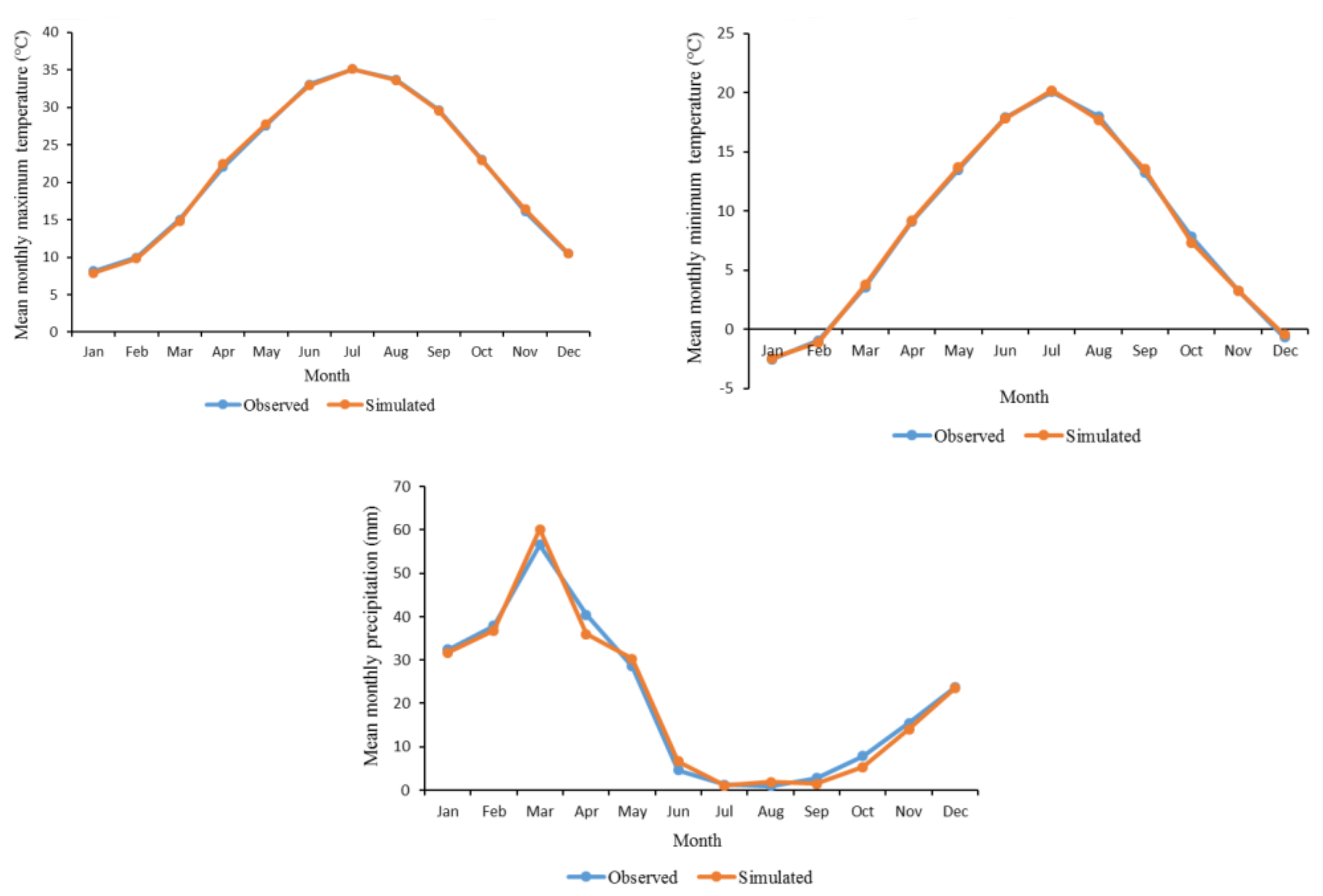
3.1. Projecting Climate Variables

Using the LARS-WG model, climatic parameters of maximum and minimum air temperature and precipitation were predicted in the Mashhad plain based on data of 1979–2016. To calibrate and ensure the accuracy of the LARS-WG model, the simulated data are compared with the observed data on a monthly scale, as shown in Figure 5. Assessment of the monthly average of maximum air temperature, minimum air temperature, and precipitation shows a good agreement among all three parameters.

LARS-WG performance also was investigated using R², NRMSE, RMSE, MAD, and MSE indicators, as presented in

Table 2. Results of LARS performance for the observed and simulated data.

Indicators	Minimum Temperature	Maximum Temperature	Precipitation
R2	0.99	0.99	0.98
NRMSE	2.55	0.95	9.96
RMSE	0.21	0.21	2.09
MAD	0.17	0.17	1.69
MSE	0.04	0.04	4.39

Sources: Research findings.

. The model successfully downscaled the minimum and maximum temperature as well as precipitation, according to the evaluation of these indicators. The higher values of R² (>0.98) and the lower values of RMSE (0.21–2.09), MAD (0.17–1.69), MSE (0.04–4.39), and NRMSE (0.95–9.96) for this period reveal that the simulated precipitation and temperature data are acceptable.

After evaluating the accuracy of the model, the climate scenarios were generated by downscaling HadGEM2 outputs under climate scenarios of RCP 2.6, 4.5, and 8.5 on the horizons of 2045. (We considered a 30-year period (2016–2045) to investigate the effects of climate change on crop production. Because the term climate is a long-term shift in the weather pattern, it is an average of at least 30 years of weather condition of a particular place [75,76,77].) The percentage change in climate variables was then calculated and compared to the benchmark year (2016). The obtained findings are shown in

Table 3. Forecasting of temperature and precipitation changes under climate scenarios in 2045 horizon compared to 2016 (benchmark year).

Scenario	Minimum Temperature	Maximum Temperature	Precipitation
RCP 2.6	3.40	4.06	−14.46
RCP 4.5	1.26	4.16	−18.14
RCP 8.5	5.88	6.05	−30.68

Note: The unit of numbers is percent.

. According to the results, the minimum and maximum temperatures are expected to increase by about 5.88% and 6.05%, respectively, while precipitation would decrease by approximately 30.68%.

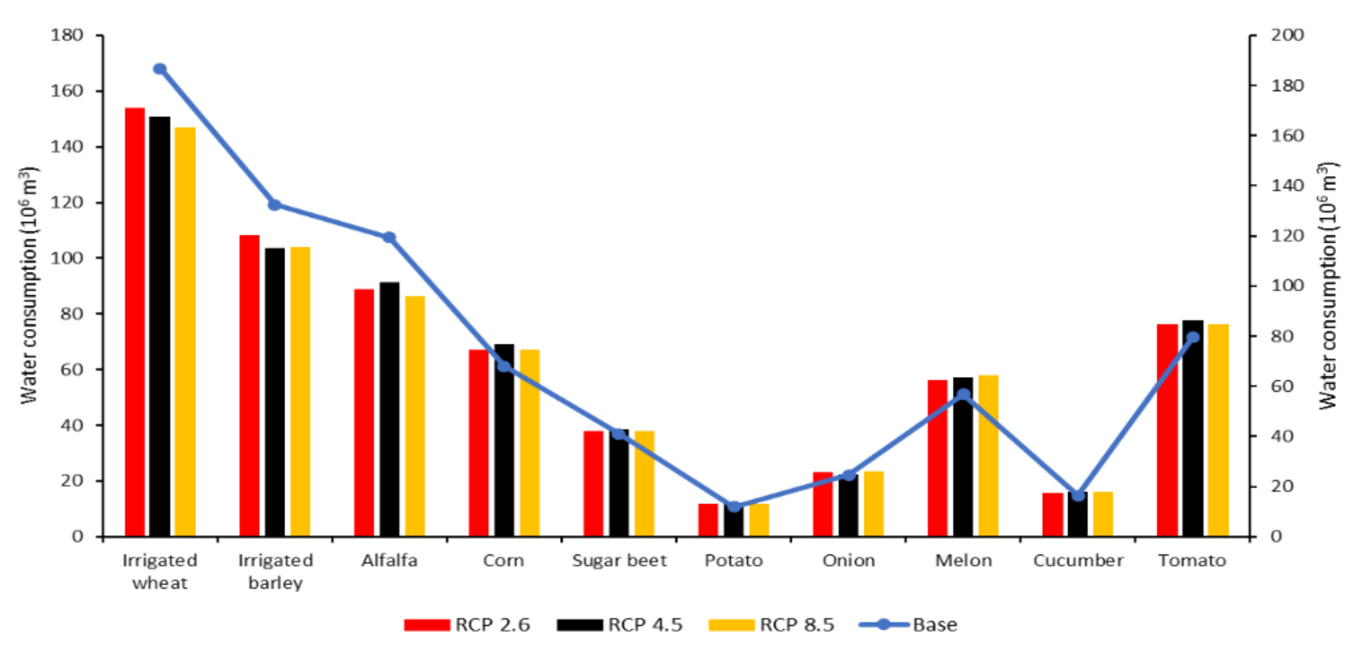
3.2. Evaluating the Impacts of Climate Change on Water Resources

The groundwater depth was forecasted because of climatic change using a panel data model under three scenarios in the Mashhad plain. The first step in the analysis was to determine whether the variables were stationary. This was performed using the Im-Pesaran-Shin (IPS) and ADF-Fisher-type panel unit root tests.

Table 4. The results of unit root test and Hausman test.

Variable	IPS		Fisher-ADF
	Without Trend	With Trend	Without Trend	With Trend
Minimum temperature	−4.57 ***	−5.03 ***	41.63 ***	31.27 ***
Maximum temperature	−4.40 ***	−5.04 ***	39.64 ***	31.31 ***
Precipitation	−18.70 ***	−19.91 ***	360.43 ***	360.43 ***
Initial groundwater depth	−13.48 ***	−13.52 ***	229.55 ***	198.43 ***
Groundwater depth	−13.50 ***	−13.53 ***	230.11 ***	198.84 ***
Fixed effects versus random effects test	Chi2		p-value
Hausman test	7.69 *		0.10

Note: * and *** show rejection of the unit root hypothesis at the 10% and 1% significance levels, respectively.

shows, for all variables in the model, the null hypothesis of unit roots is rejected with a 99% confidence level. As a result, the model’s variables were all stationary. For panel data, the random-effects and fixed-effects models were used. To identify which should be used, the Hausman test was used. As shown in Table 4, the null hypothesis of no correlation between regional effects and independent variables is rejected. As a result, a fixed-effect model with regional-specific effects was used.

The results of the panel data model for sensitivity of the groundwater depth to climate variables are presented in

Table 5. Sensitivity of the groundwater depth to minimum and maximum temperatures and precipitation in the study area.

Variable	Coefficient	T-Statistic	P-value
Minimum temperature	0.003	0.31	0.75
Maximum temperature	0.003	0.26	0.79
Precipitation	−0.001 *	−1.69	0.09
Initial groundwater depth	0.99 ***	249.04	0.00
Constant	0.40 *	1.79	0.07

* and ***, respectively, indicate rejection of the unit root hypothesis at the 10% and 1% significance levels.

. The findings indicated that maximum and minimum temperatures had a positive impact on the groundwater depth in the Mashhad plain from 2000 to 2016. Furthermore, precipitation was negatively and significantly related to groundwater depth in the plain. Therefore, as precipitation increased, the groundwater depth decreased, resulting in more water in the well, according to many previous studies, including Shahvari et al. [28] and Izady et al. [41].

The results regarding the percentage changes in groundwater depth and water availability under climatic scenarios compared to the baseline are presented in

Table 6. Percentage change in groundwater depth and water availability in the study area under climate scenarios compared to the baseline.

Scenario	Groundwater Depth	Water Availability
RCP 2.6	13.79	−13.25
RCP 4.5	13.50	−13.26
RCP 8.5	15.45	−14.84

Sources: Research findings.

. According to the findings, the depth of groundwater in the Mashhad plain is expected to rise about 13.79% in RCP 2.6, 13.50% in RCP 4.5, and 15.45% in RCP 8.5. Furthermore, water availability will increase by approximately 13.25%, 13.26%, and 14.84% in response to RCP 2.6, RCP 4.5, and RCP 8.5, respectively.

3.3. Assessing the Impacts of Climate Change on Crop Yield

To assess crop yield sensitivity to temperature and precipitation, the yield response function was estimated using the GME model. The estimated results are displayed in

Table 7. Estimates of the impact of climatic variables on crop yield using the GME model.

Crop	Minimum Temperature	Minimum Temperature	Precipitation	Trend	Constant
Irrigated wheat	−1.17 * (0.64)	0.76 *** (0.19)	0.17 ** (0.08)	0.009 ** (0.004)	9.16 *** (1.92)
Rainfed wheat	−0.53 (1.35)	0.93 ** (0.40)	0.49 *** (0.18)	0.004 (0.008)	4.20 (4.07)
Irrigated barley	−0.68 (0.71)	0.71 *** (0.16)	0.13 * (0.07)	0.002 (0.003)	8.09 *** (1.64)
Rainfed barley	−1.22 (1.12)	1.06 *** (0.34)	0.14 (0.15)	0.003 (0.007)	7.42 ** (3.35)
Alfalfa	−2.82 *** (0.77)	−0.62 (0.31)	0.07 (0.06)	0.01 *** (0.004)	18.61 *** (2.41)
Corn	2.37 *** (0.96)	−0.08 (0.41)	0.06 *** (0.02)	0.007 * (0.003)	2.57 (3.42)
Sugar beet	0.62 (0.75)	−1.19 *** (0.36)	0.09 ** (0.04)	0.02 *** (0.003)	10.61 *** (2.62)
Potato	0.53 (1.75)	−0.93 (0.93)	−0.10 (0.07)	0.03 ***(0.007)	10.30 * (5.94)
Onion	−3.16 ** (1.47)	1.55 * (0.89)	−0.11 (0.09)	0.03 *** (0.006)	16.26 *** (4.77)
Melon	1.61 *** (0.64)	−0.85 ** (0.38)	0.11 *** (0.04)	0.01 *** (0.003)	5.88 *** (2.05)
Cucumber	1.99 (1.39)	−2.94 *** (0.96)	0.11 *** (0.05)	0.02 *** (0.006)	10.38 ** (4.62)
Tomato	1.20 (0.86)	−0.90 ** (0.46)	0.08 * (0.05)	0.02 *** (0.003)	7.95 *** (2.90)

Note: Numbers in parenthesis indicate standard error. *, **, and ***, respectively, indicate rejection of the unit root hypothesis at the 10%, 5%, and 1% significance levels.

. The Cobb–Douglas functional form was used in the estimation of yield response functions. Therefore, the estimated parameters in Table 5 show the elasticity values. Based on the results obtained from this table, increasing maximum and minimum temperatures reduce crop yield in many crops. In the case of irrigated wheat, for example, the results show that a 1% increase in maximum temperature results in a 1.17% decrease in yield. In addition, a 1% increase in the minimum temperature increases irrigated wheat yield by approximately 0.76%. Precipitation has a negative impact on yield of some crops due to increase humidity or the potential spread of diseases and pests [78]. Irrigated wheat, rainfed wheat, irrigated barley, rainfed barley, alfalfa, corn, sugar beet, melon, cucumber, and tomato yield are positively influenced by precipitation.

The percentage changes in crop yield in the Mashhad plain under RCP 2.6, RCP 4.5, and RCP 8.5 on the horizon in 2045, as compared to the baseline year, are presented in

Table 8. Percentage changes in crop yield under RCP 2.6, RCP 4.5, and RCP 8.5 for 2045, as compared to the base period in the Mashhad plain.

Crop	RCP 2.6	RCP 4.5	RCP 8.5
Irrigated wheat	−8.71	−11.32	−13.57
Rainfed wheat	−14.48	−18.34	−17.29
Irrigated barley	−5.21	−7.90	−8.56
Rainfed barley	−7.17	−11.04	−12.92
Alfalfa	−19.83	−19.07	−25.20
Corn	13.33	15.64	10.11
Sugar beet	−1.75	−0.98	−5.86
Potato	3.53	5.33	4.74
Onion	−8.86	−14.41	−10.46
Melon	3.12	5.92	5.12
Cucumber	−7.71	−3.91	−8.29
Tomato	2.34	4.02	0.15

Sources: Research findings.

. The findings imply that the yield of irrigated wheat, rainfed wheat, irrigated barley, rainfed barley, alfalfa, sugar beet, onion, and cucumber will decrease in response to all three climate scenarios. Alfalfa crop is prone to experience a decrease in yield between 19.07% and 25.20% and is expected to emerge as a highly vulnerable crop in 2045. In addition, climate change will increase the yield of corn, potato, melon, and tomato crops under all scenarios. With changing climate, corn yield will rise more than other crops. This result is in line with the results of Almaraz et al. [79] and Zhang et al. [80].

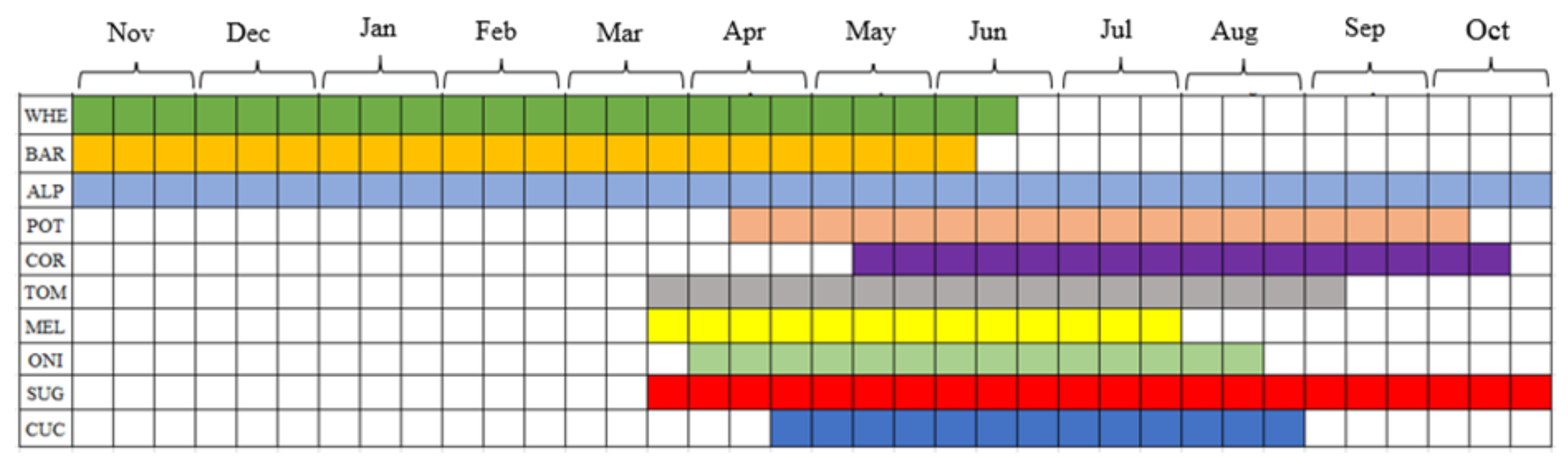
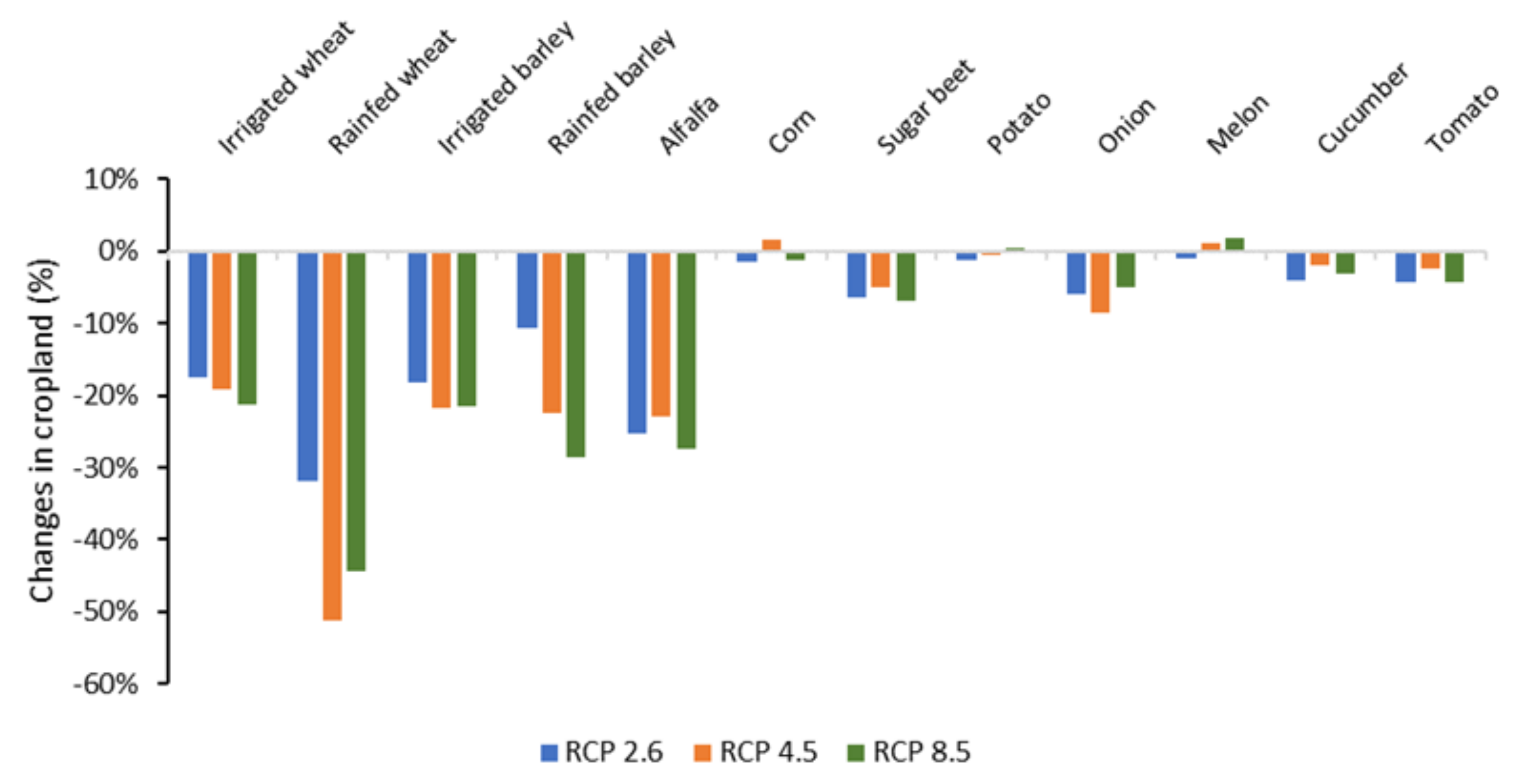
3.4. Evaluating the Impacts of Climate Change on Crop Production and Cropping Pattern

In this section, changes in crop yields and water availability under climate change were incorporated into the PMP model to assess the impact of climate change on cropping pattern, crop production, and water consumption. It is worth noting that the cropping pattern is defined as a combination of agricultural crops that are grown in a particular geographical area [81]. The percentage changes in cropland under three climate scenarios in 2045, as compared to the base year, are shown in Figure 6. The results imply that RCP 2.6, RCP 4.5, and RCP 8.5 scenarios will decrease the cultivated area of irrigated wheat, rainfed wheat, irrigated barley, rainfed barley, alfalfa, sugar beet, onion, cucumber, and tomato in 2045 in the Mashhad plain. On the contrary, the cultivated area of corn, potato, and melon will increase under two scenarios of RCP 4.5 and RCP 8.5 in 2045 relative to the base year. As shown in the figure, the most significant reduction in cultivated land is related to rainfed wheat and RCP 4.5, where the area under cultivation will reduce by approximately 51.16%.

The percentage changes in crop production under climate scenarios for 2045, as compared to the baseline, are presented in

Table 9. Percentage changes in crop production under RCP 2.6, RCP 4.5, and RCP 8.5 for 2045 as compared to the base year in the Mashhad plain.

Crop	RCP 2.6	RCP 4.5	RCP 8.5
Irrigated wheat	−24.95	−28.08	−32.36
Rainfed wheat	−41.43	−59.95	−53.75
Irrigated barley	−22.21	−28.05	−28.50
Rainfed barley	−16.98	−30.96	−37.94
Alfalfa	−40.24	−37.66	−45.53
Corn	11.37	17.92	8.61
Sugar beet	−8.28	−5.85	−12.54
Potato	2.64	4.41	5.33
Onion	−14.51	−21.42	−14.40
Melon	2.05	7.14	6.90
Cucumber	−11.77	−5.90	−10.80
Tomato	−2.41	1.40	−4.12

Sources: Research findings.

. The results of this table show that production of crops, such as irrigated wheat, rainfed wheat, irrigated barley, rainfed barley, alfalfa, sugar beet, onion, and cucumber, will decrease in response to all three climate scenarios. Therefore, the biggest decline (59.95%) will occur for rainfed wheat in RCP 4.5 scenario.

In addition, corn, potato, and melon production will increase by about 17.92%, 5.33%, and 7.14%, respectively, under climate scenarios. This increase in production is due to an increase in yield or area under cultivation, or both, as discussed in the previous section. Additionally, in the presence of climate change in 2045, the Mashhad plain will experience the biggest increase in crop production in corn and RCP 4.5.

Given the decline in production of most crops that account for a large share of the region’s production, it is reasonable to conclude that the occurrence of climate change poses a serious threat to crop production and food security in the region.

Figure 7 shows the water consumption for each crop under current conditions and different climatic scenarios. As expected, under climate scenarios, due to the reduction in water availability and crop yield and, consequently, reduced cropland, water consumption will decrease for crops, such as irrigated wheat (21.40%), irrigated barley (21.88%), alfalfa (27.70%), sugar beet (7.90%), onion (8.71%), cucumber (4.52%), and tomato (4.33%), while there is an increase in water consumption for corn, potato, and melon because of improved yield. Overall, it can be stated that water consumption in climatic scenarios will be reduced by about 13.30%, 13.31%, and 14.90% under RCP 2.6, RCP 4.5, and RCP 8.5, respectively, compared to baseline conditions.

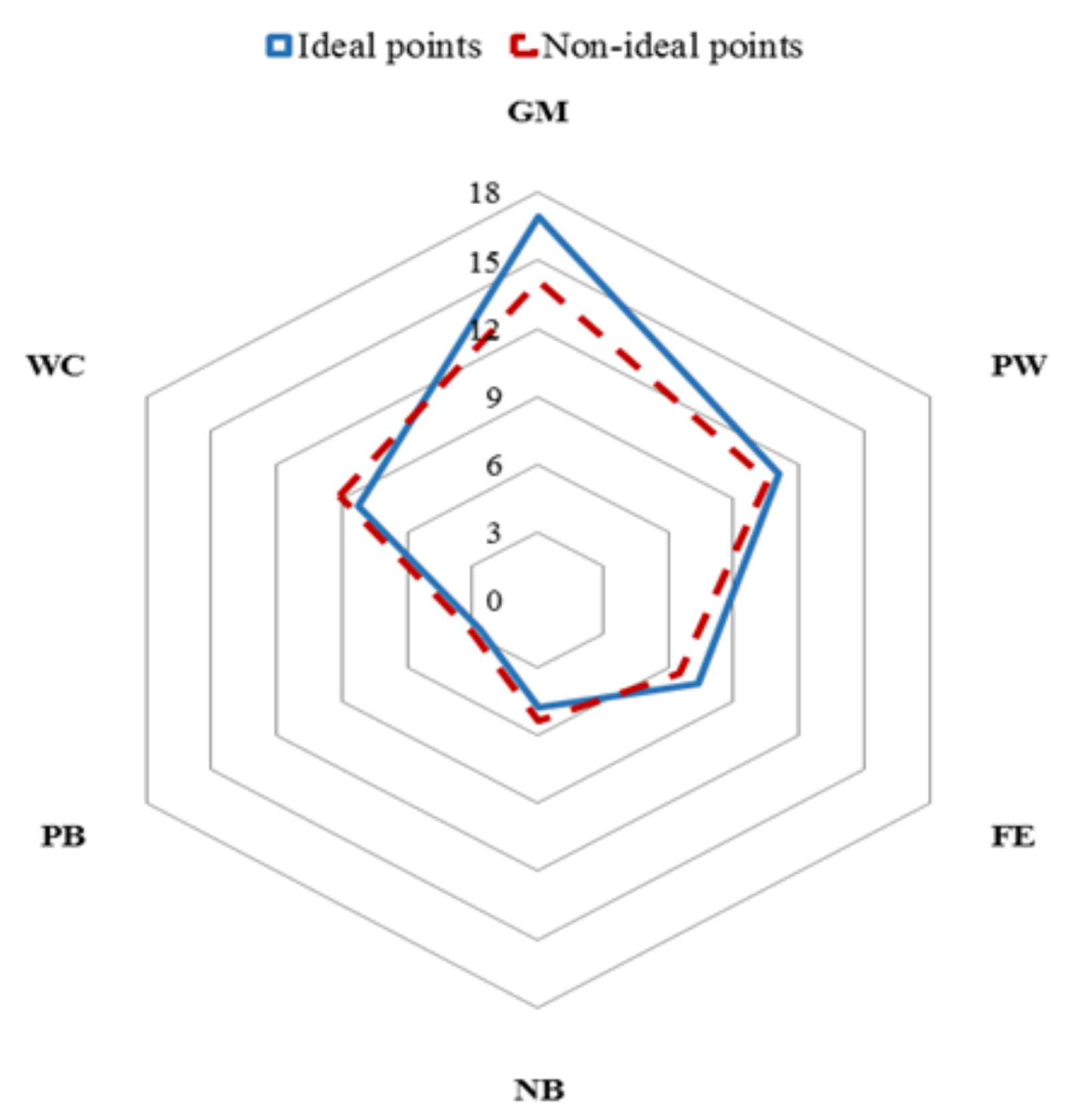
3.5. Assessing the Impacts of Climate Change on Agricultural Sustainability

In the present study, an attempt has been made to evaluate the effects of climate change on agricultural sustainability in the study area using the TOPSIS approach. In the first step, we employed the AHP method to determine the weight of indicators and sub-indicators through interviews with 15 agricultural experts and specialists.

Table 10. Selected indicators and weights.

Indicator	Weights of Criteria (%)	Sub-Indicator	Measurement Unit	Weights of Indicator (%)	Normalized Weights of Indicator (%)	Polarity of Indicator
Economic	52.43	GM	MT	58.33	30.58	+
		PW	MT/103 m3	41.67	21.85	+
Social	14.10	FE	h/ha	100.00	14.10	+
Environmental	33.47	NB	kg/ha	30.51	10.21	−
		PB	kg/ha	17.16	5.74	−
		WC	103 m3/ha	52.33	17.52	−

Note: MT is million tomans.

shows the weights assigned to each indicator and sub-indicator. According to the results of this table, economic, environmental, and social indicators have the greatest importance with 52%, 33%, and 14%, respectively. Due to the low income of farmers in Iran, improving the profitability of agricultural activities is critical to achieving sustainable development in the agricultural sector [60]. In addition, over the past few decades, the excessive use of chemical fertilizers and the uncontrolled extraction of groundwater resources in the process of food production in agriculture has caused irreversible environmental damage [16]. This highlights the importance of environmental issues in assessing the sustainability of Iran’s agricultural sector. In the economic indicator, the importance of the “GM” and “PW” sub-indicators are 58% and 42%, respectively. Because of Iran’s high unemployment rate, the FE index was deemed as the mere social indicator, with a weight of 14%. Among the environmental sub-indicators, WC is the most important environmental sub-indicator, followed by the NI and PB.

In the second step, using the results obtained from the PMP model, the value of each of the sustainability indicators in the base conditions and climatic scenarios was calculated, which forms the decision matrix (see

Table 11. Decision matrix.

Alternative	GM	PW	FE	NB	PB	WC
Base	316,270.25	0.43	162.05	153.34	81.55	8.36
RCP 2.6	279,714.25	0.44	173.04	163.50	86.50	8.72
RCP 4.5	278,643.55	0.44	183.86	172.13	91.12	9.26
RCP 8.5	262,996.33	0.42	182.28	171.21	90.53	9.15

Sources: Research findings.

). Table 11 shows under the climate scenarios that the values of economic indicators are lower and environmental indicators are higher than the baseline conditions.

Table 12. Normalized decision matrix.

Alternative	GM	PW	FE	NB	PB	WC
Base	0.55	0.50	0.46	0.46	0.47	0.47
RCP 2.6	0.49	0.51	0.49	0.49	0.49	0.49
RCP 4.5	0.49	0.51	0.52	0.52	0.52	0.52
RCP 8.5	0.46	0.49	0.52	0.52	0.52	0.52

Sources: Research findings.

indicates the normalized decision matrix. Figure 8 depicts the distribution of positive and negative ideal options across the various sustainability indicators. In the final step, current and climatic conditions were ranked based on sustainability indicators (see

Table 13. Ranking of alternatives.

Alternative	Ci	Rank
Base	0.77	1
RCP 2.6	0.38	2
RCP 4.5	0.36	3
RCP 8.5	0.21	4

Sources: Research findings.

). Based on the results of Table 13, the base condition has the highest Ci values (0.77), indicating that the phenomenon of climate change can be considered a serious threat to the agricultural sustainability in this region. The findings in this section of the research are in line with the study of Karandish et al. [82] and Ghanian et al. [83].

To ensure consistency in the results of Table 13, a sensitivity analysis of the economic, social, and environmental criteria weights used in the TOPSIS model is performed. To achieve this goal, a total of seven experiments has been conducted to compare the impact of potential changes in the weights of economic, social, and environmental criteria (see

Table 14. Results of the sensitivity analysis.

Experiment		Best Alternative
1	All Sub-indicators have same weight	Base
2	Weight of GM criterion = 50% Weight of the other criteria = 10%	Base
3	Weight of PW criterion = 50% Weight of the other criteria = 10%	Base
4	Weight of FE criterion = 50% Weight of the other criteria = 10%	RCP 4.5
5	Weight of NB criterion = 50% Weight of the other criteria = 10%	Base
6	Weight of PB criterion = 50% Weight of the other criteria = 10%	Base
7	Weight of WC criterion = 50% Weight of the other criteria = 10%	Base

). In Experiment 1, all sub-indicators have the same weight (16.66%); in Experiment 2–7, the weight of one criterion is higher than the weight of the remaining criteria. The results of the sensitivity analysis described indicate that in all experiments (except Experiment 4), the base condition is selected as the best alternative. In other words, given the importance of economic and environmental indicators in Iran’s agricultural sector, it is reasonable to expect that if the harmful effects of climate change are not properly managed, the phenomenon will have a negative impact on agricultural sustainability.

4. Conclusions

The climate simulation model predicted a 6% increase in minimum and maximum temperatures, as well as a 30% decrease in precipitation. Additionally, the results showed that water availability will decrease between 13% and 15% under different climate scenarios. Crop yields were found to be negatively affected by increasing maximum and minimum temperatures. Precipitation affects crop yield in different ways, with positive effects on irrigated wheat, rainfed wheat, irrigated barley, rainfed barley, alfalfa, corn, sugar beet, melon, cucumber, and tomato yields and negative effects on potato and onion yields. Overall, future climate change is expected to reduce the yield of irrigated wheat, rainfed wheat, irrigated barley, rainfed barley, alfalfa, sugar beet, onion, and cucumber, while the effects will be reversed for corn, potato, melon, and tomato. The results of the PMP model showed that changes in crops yield and water availability will lead to a reduction in the cultivated area of most crops in 2045, among which dryland wheat will experience the greatest decrease (51%). The results of the evaluation of the effects of climate change on agricultural sustainability show that this phenomenon can have adverse economic and environmental effects on the agricultural system of the study area. As a result, it can have a negative impact on agricultural sustainability if not properly managed.

In entirety, the findings of this study reflect the fact that water and food security in the region will be severely adversely affected by climate change in the future. Nevertheless, by continuing to support population growth policies, uncontrolled extraction of groundwater, and expansion of urbanization in the presence of climate change, more severe irreversible effects on water and food resources in the control area are expected. These results underscore the necessity of implementing adaptation policies, such as reforming the cropping pattern and production technologies, as well as the introduction of drought-tolerant varieties to reduce the detrimental effects of climate in the region.

References

1. Alkaya, E.; Bogurcu, M.; Ulutas, F.; Demirer, G.N. Adaptation to climate change in industry: Improving resource efficiency through sustainable production applications. Water Environ. Res. 2015, 87, 14–25. [Google Scholar] [CrossRef] [PubMed] [Green Version]
2. Shayanmehr, S.; Rastegari Henneberry, S.; Sabouhi Sabouni, M.; Shahnoushi Foroushani, N. Climate Change and Sustainability of Crop Yield in Dry Regions Food Insecurity. Sustainability 2020, 12, 9890. [Google Scholar] [CrossRef]
3. Chiu, S.-Y.; Kao, C.-Y.; Tsai, M.-T.; Ong, S.-C.; Chen, C.-H.; Lin, C.-S. Lipid accumulation and CO2 utilization of Nannochloropsis oculata in response to CO2 aeration. Bioresour. Technol. 2009, 100, 833–838. [Google Scholar] [CrossRef] [PubMed]
4. Gao, M.; Yang, H.; Xiao, Q.; Goh, M. A novel fractional grey Riccati model for carbon emission prediction. J. Clean. Prod. 2021, 282, 124471. [Google Scholar] [CrossRef]
5. Gao, M.; Yang, H.; Xiao, Q.; Goh, M. A novel method for carbon emission forecasting based on Gompertz’s law and fractional grey model: Evidence from American industrial sector. Renew. Energy 2022, 181, 803–819. [Google Scholar] [CrossRef]
6. Noh, S.; Son, Y.; Park, J. Life cycle carbon dioxide emissions for fill dams. J. Clean. Prod. 2018, 201, 820–829. [Google Scholar] [CrossRef]
7. Radmehr, R.; Henneberry, S.R.; Shayanmehr, S. Renewable energy consumption, CO2 emissions, and economic growth nexus: A simultaneity spatial modeling analysis of EU countries. Struct. Change Econ. Dyn. 2021, 57, 13–27. [Google Scholar] [CrossRef]
8. Kohansal, M.R.; Shayan, M.S. The interplay between energy consumption, economic growth and environmental pollution: Application of spatial panel simultaneous-equations model. Iran. Energy Econ. 2016, 5, 179–216. [Google Scholar]
9. Hezareh, R.; Shayanmehr, S.; Darbandi, E.; Schieffer, J. Energy Consumption and Environmental Pollution: Evidence from the Spatial Panel Simultaneous-Equations Model of Developing Countries; Southern Agricultural Economics Association (SAEA): Birmingham, AL, USA, 2017. [Google Scholar]
10. Jin, S.; Hao, Z.; Zhang, K.; Yan, Z.; Chen, J. Advances and challenges for the electrochemical reduction of CO2 to CO: From fundamentals to industrialization. Angew. Chem. Int. Ed. 2021, 60, 20627–20648. [Google Scholar] [CrossRef]
11. Anjum, S.A.; Farooq, M.; Xie, X.-Y.; Liu, X.-J.; Ijaz, M.F. Antioxidant defense system and proline accumulation enables hot pepper to perform better under drought. Sci. Hortic. 2012, 140, 66–73. [Google Scholar] [CrossRef]
12. Kiani Ghalehsard, S.; Shahraki, J.; Akbari, A.; Sardar Shahraki, A. Assessment of the impacts of climate change and variability on water resources and use, food security, and economic welfare in Iran. Environ. Dev. Sustain. 2021, 23, 14666–14682. [Google Scholar] [CrossRef]
13. Sabbaghi, M.A.; Nazari, M.; Araghinejad, S.; Soufizadeh, S. Economic impacts of climate change on water resources and agriculture in Zayandehroud river basin in Iran. Agric. Water Manag. 2020, 241, 106323. [Google Scholar] [CrossRef]
14. Varela Ortega, C.; Esteve, P.; Blanco, I.; Carmona, G.; Ruiz Fernández, J.; Rabah, T. Assessment of Socio-Economic and Climate Change Effects on Water Resources and Agriculture in Southern and Eastern Mediterranean Countries. MEDPRO Technical Report. 2013. Available online: https://ssrn.com/abstract=2276859 (accessed on 10 June 2022).
15. Lehmann, N.; Finger, R.; Klein, T.; Calanca, P.; Walter, A. Adapting crop management practices to climate change: Modeling optimal solutions at the field scale. Agric. Syst. 2013, 117, 55–65. [Google Scholar] [CrossRef]
16. Palazzoli, I.; Maskey, S.; Uhlenbrook, S.; Nana, E.; Bocchiola, D. Impact of prospective climate change on water resources and crop yields in the Indrawati basin, Nepal. Agric. Syst. 2015, 133, 143–157. [Google Scholar] [CrossRef]
17. Connolly-Boutin, L.; Smit, B. Climate change, food security, and livelihoods in sub-Saharan Africa. Reg. Environ. Change 2016, 16, 385–399. [Google Scholar] [CrossRef] [Green Version]
18. Ahmadi, H.; Ghalhari, G.F.; Baaghideh, M. Impacts of climate change on apple tree cultivation areas in Iran. Clim. Change 2019, 153, 91–103. [Google Scholar] [CrossRef]
19. Perdinan, P. A Rationale for International Cooperation in Implementing Adaptation Strategies to Climate Change in the Face of Global Inequality. J. Indones. Focus 2010, 1, 1–8. [Google Scholar]
20. Jat, M.L.; Stirling, C.M.; Jat, H.S.; Tetarwal, J.P.; Jat, R.K.; Singh, R.; Lopez-Ridaura, S.; Shirsath, P.B. Soil processes and wheat cropping under emerging climate change scenarios in South Asia. Adv. Agron. 2018, 148, 111–171. [Google Scholar]
21. Radmehr, R.; Ghorbani, M.; Ziaei, A.N. Quantifying and managing the water-energy-food nexus in dry regions food insecurity: New methods and evidence. Agric. Water Manag. 2021, 245, 106588. [Google Scholar] [CrossRef]
22. Mosavi, S.H.; Soltani, S.; Khalilian, S. Coping with climate change in agriculture: Evidence from Hamadan-Bahar plain in Iran. Agric. Water Manag. 2020, 241, 106332. [Google Scholar] [CrossRef]
23. Shayanmehr, S.; Shahnoushi, N.; Sabouhi Sabouni, M.; Rastegari, S. Climate Change and Its Consequences on Food Security in Khorasan Region. Agric. Econ. 2021, 15, 95–128. [Google Scholar]
24. Xiong, W.; Holman, I.; Lin, E.; Conway, D.; Jiang, J.; Xu, Y.; Li, Y. Climate change, water availability and future cereal production in China. Agric. Ecosyst. Environ. 2010, 135, 58–69. [Google Scholar] [CrossRef]
25. Sinnarong, N.; Chen, C.-C.; McCarl, B.; Tran, B.-L. Estimating the potential effects of climate change on rice production in Thailand. Paddy Water Environ. 2019, 17, 761–769. [Google Scholar] [CrossRef]
26. Mostafa, S.M.; Wahed, O.; El-Nashar, W.Y.; El-Marsafawy, S.M.; Abd-Elhamid, H.F. Impact of climate change on water resources and crop yield in the Middle Egypt region. AQUA—Water Infrastruct. Ecosyst. Soc. 2021, 70, 1066–1084. [Google Scholar] [CrossRef]
27. Medellín-Azuara, J.; Howitt, R.E.; MacEwan, D.J.; Lund, J.R. Economic impacts of climate-related changes to California agriculture. Clim. Change 2011, 109, 387–405. [Google Scholar] [CrossRef]
28. Shahvari, N.; Khalilian, S.; Mosavi, S.H.; Mortazavi, S.A. Assessing climate change impacts on water resources and crop yield: A case study of Varamin plain basin, Iran. Environ. Monit. Assess. 2019, 191, 134. [Google Scholar] [CrossRef]
29. Lu, S.; Bai, X.; Li, W.; Wang, N. Impacts of climate change on water resources and grain production. Technol. Forecast. Soc. Chang. 2019, 143, 76–84. [Google Scholar] [CrossRef]
30. Khashei-Siuki, A.; Sarbazi, M. Evaluation of ANFIS, ANN, and geostatistical models to spatial distribution of groundwater quality (case study: Mashhad plain in Iran). Arab. J. Geosci. 2015, 8, 903–912. [Google Scholar] [CrossRef]
31. Toosi, A.S.; Doulabian, S.; Tousi, E.G.; Calbimonte, G.H.; Alaghmand, S. Large-scale flood hazard assessment under climate change: A case study. Ecol. Eng. 2020, 147, 105765. [Google Scholar] [CrossRef]
32. Naghibi, S.A.; Vafakhah, M.; Hashemi, H.; Pradhan, B.; Alavi, S.J. Groundwater augmentation through the site selection of floodwater spreading using a data mining approach (case study: Mashhad Plain, Iran). Water 2018, 10, 1405. [Google Scholar] [CrossRef] [Green Version]
33. Wilks, D.S.; Wilby, R.L. The weather generation game: A review of stochastic weather models. Prog. Phys. Geogr. 1999, 23, 329–357. [Google Scholar] [CrossRef]
34. Tashekaboud, S.H.; Heydari Tashekaboud, A. Investigating the effects of climate change on stream flows of Urmia Lake basin in Iran. Modeling Earth Syst. Environ. 2019, 329–339. [Google Scholar]
35. Kilsby, C.G.; Jones, P.; Burton, A.; Ford, A.; Fowler, H.J.; Harpham, C.; James, P.; Smith, A.; Wilby, R. A daily weather generator for use in climate change studies. Environ. Model. Softw. 2007, 22, 1705–1719. [Google Scholar] [CrossRef]
36. Racsko, P.; Szeidl, L.; Semenov, M. A serial approach to local stochastic weather models. Ecol. Model. 1991, 57, 27–41. [Google Scholar] [CrossRef]
37. Semenov, M.A.; Brooks, R.J.; Barrow, E.M.; Richardson, C.W. Comparison of the WGEN and LARS-WG stochastic weather generators for diverse climates. Clim. Res. 1998, 10, 95–107. [Google Scholar] [CrossRef] [Green Version]
38. Ahmadi, M.; Etedali, H.R.; Elbeltagi, A. Evaluation of the effect of climate change on maize water footprint under RCPs scenarios in Qazvin plain, Iran. Agric. Water Manag. 2021, 254, 106969. [Google Scholar] [CrossRef]
39. Baez-Villanueva, O.M.; Zambrano-Bigiarini, M.; Ribbe, L.; Nauditt, A.; Giraldo-Osorio, J.D.; Thinh, N.X. Temporal and spatial evaluation of satellite rainfall estimates over different regions in Latin-America. Atmos. Res. 2018, 213, 34–50. [Google Scholar] [CrossRef]
40. Zarei, A.; Chemura, A.; Gleixner, S.; Hoff, H. Evaluating the grassland NPP dynamics in response to climate change in Tanzania. Ecol. Indic. 2021, 125, 107600. [Google Scholar] [CrossRef]
41. Izady, A.; Davary, K.; Alizadeh, A.; Ghahraman, B.; Sadeghi, M.; Moghaddamnia, A. Application of “panel-data” modeling to predict groundwater levels in the Neishaboor Plain, Iran. Hydrogeol. J. 2012, 20, 435–447. [Google Scholar] [CrossRef] [Green Version]
42. Arellano, M. Panel Data Econometrics; OUP Oxford: Oxford, UK, 2003. [Google Scholar]
43. Chinnasamy, P.; Maheshwari, B.; Dillon, P.; Purohit, R.; Dashora, Y.; Soni, P.; Dashora, R. Estimation of specific yield using water table fluctuations and cropped area in a hardrock aquifer system of Rajasthan, India. Agric. Water Manag. 2018, 202, 146–155. [Google Scholar] [CrossRef]
44. Asoka, A.; Gleeson, T.; Wada, Y.; Mishra, V. Relative contribution of monsoon precipitation and pumping to changes in groundwater storage in India. Nat. Geosci. 2017, 10, 109–117. [Google Scholar] [CrossRef] [Green Version]
45. Rohde, M.M.; Edmunds, W.M.; Freyberg, D.; Sharma, O.P.; Sharma, A. Estimating aquifer recharge in fractured hard rock: Analysis of the methodological challenges and application to obtain a water balance (Jaisamand Lake Basin, India). Hydrogeol. J. 2015, 23, 1573–1586. [Google Scholar] [CrossRef]
46. Shayannmehr, S. Climate Change and Its Impacts on Major Crops Production and Market in Iran; Ferdowsi University of Mashhad: Mashhad, Iran, 2021. [Google Scholar]
47. Shayanmehr, S.; Rastegari Henneberry, S.; Sabouhi Sabouni, M.; Shahnoushi Foroushani, N. Drought, climate change, and dryland wheat yield response: An econometric approach. Int. J. Environ. Res. Public Health 2020, 17, 5264. [Google Scholar] [CrossRef]
48. Attavanich, W.; McCarl, B.A. The Effect of Climate Change, CO2 Fertilization, and Crop Production Technology on Crop Yields and Its Economic Implications on Market Outcomes and Welfare Distribution; Agricultural & Applied Economics Association: Philadelphia, PA, USA, 2011. [Google Scholar]
49. Baltagi, B.H. Econometric Analysis of Panel Data; John Wiley & Sons Ltd.: West Sussex, UK, 2005. [Google Scholar]
50. Golan, A.; Judge, G.; Karp, L. A maximum entropy approach to estimation and inference in dynamic models or counting fish in the sea using maximum entropy. J. Econ. Dyn. Control 1996, 20, 559–582. [Google Scholar] [CrossRef]
51. Moreno, B.; García-Álvarez, M.T.; Ramos, C.; Fernández-Vázquez, E. A General Maximum Entropy Econometric approach to model industrial electricity prices in Spain: A challenge for the competitiveness. Appl. Energy 2014, 135, 815–824. [Google Scholar] [CrossRef]
52. Liu, W.; Radmehr, R.; Zhang, S.; Henneberry, S.R.; Wei, C. Driving mechanism of concentrated rural resettlement in upland areas of Sichuan Basin: A perspective of marketing hierarchy transformation. Land Use Policy 2020, 99, 104879. [Google Scholar] [CrossRef]
53. Qureshi, M.E.; Whitten, S.M.; Kirby, M. A multi-period positive mathematical programming approach for assessing economic impact of drought in the Murray–Darling Basin, Australia. Econ. Model. 2014, 39, 293–304. [Google Scholar] [CrossRef]
54. Fathelrahman, E.; Davies, A.; Davies, S.; Pritchett, J. Assessing climate change impacts on water resources and Colorado agriculture using an equilibrium displacement mathematical programming model. Water 2014, 6, 1745–1770. [Google Scholar] [CrossRef] [Green Version]
55. Elouadi, D.; Ouazar, M.; Doukkali, L.; Elyoussfi, A. A mathematical model for assessment of socio-economic impact of climate change on agriculture activities: Cases of the east of Morocco (africa). Indian J. Sci. Technol. 2017, 10, 1–6. [Google Scholar] [CrossRef]
56. Zhao, Z.; Wang, G.; Chen, J.; Wang, J.; Zhang, Y. Assessment of climate change adaptation measures on the income of herders in a pastoral region. J. Clean. Prod. 2019, 208, 728–735. [Google Scholar] [CrossRef]
57. Henderson, B.; Cacho, O.; Thornton, P.; van Wijk, M.; Herrero, M. The economic potential of residue management and fertilizer use to address climate change impacts on mixed smallholder farmers in Burkina Faso. Agric. Syst. 2018, 167, 195–205. [Google Scholar] [CrossRef]
58. Laskookalayeh, S.S.; Najafabadi, M.M.; Shahnazari, A. Investigating the effects of management of irrigation water distribution on farmers’ gross profit under uncertainty: A new positive mathematical programming model. J. Clean. Prod. 2022, 351, 131277. [Google Scholar] [CrossRef]
59. Radmehr, R.; Shayanmehr, S. The determinants of sustainable irrigation water prces in Iran. Bulg. J. Agric. Sci 2018, 24, 893–919. [Google Scholar]
60. Radmehr, R.; Ghorbani, M.; Kulshreshtha, S. Selecting strategic policy for irrigation water management (Case Study: Qazvin Plain, Iran). J. Agric. Sci. Technol. 2020, 22, 579–593. [Google Scholar]
61. Röhm, O.; Dabbert, S. Integrating agri-environmental programs into regional production models: An extension of positive mathematical programming. Am. J. Agric. Econ. 2003, 85, 254–265. [Google Scholar] [CrossRef]
62. Paris, Q.; Howitt, R.E. An analysis of ill-posed production problems using maximum entropy. Am. J. Agric. Econ. 1998, 80, 124–138. [Google Scholar] [CrossRef]
63. Gallego-Ayala, J. Selecting irrigation water pricing alternatives using a multi-methodological approach. Math. Comput. Model. 2012, 55, 861–883. [Google Scholar] [CrossRef]
64. Orojloo, M.; Shahdany, S.M.H.; Roozbahani, A. Developing an integrated risk management framework for agricultural water conveyance and distribution systems within fuzzy decision making approaches. Sci. Total Environ. 2018, 627, 1363–1376. [Google Scholar] [CrossRef]
65. Mortazavi, S.A.; Hezareh, R.; Ahmadi Kaliji, S.; Shayan Mehr, S. Application of linear and non-linear programming model to assess the sustainability of water resources in agricultural patterns. Int. J. Agric. Manag. Dev. 2014, 4, 27–32. [Google Scholar]
66. Kalbar, P.P.; Karmakar, S.; Asolekar, S.R. Technology assessment for wastewater treatment using multiple-attribute decision-making. Technol. Soc. 2012, 34, 295–302. [Google Scholar] [CrossRef]
67. Balioti, V.; Tzimopoulos, C.; Evangelides, C. Multi-criteria decision making using TOPSIS method under fuzzy environment. Application in spillway selection. Multidiscip. Digit. Publ. Inst. Proc. 2018, 2, 637. [Google Scholar]
68. Durmuşoğlu, Z.D.U. Assessment of techno-entrepreneurship projects by using Analytical Hierarchy Process (AHP). Technol. Soc. 2018, 54, 41–46. [Google Scholar] [CrossRef]
69. Rao, C.; Gao, M.; Wen, J.; Goh, M. Multi-attribute group decision making method with dual comprehensive clouds under information environment of dual uncertain Z-numbers. Inf. Sci. 2022, 602, 106–127. [Google Scholar] [CrossRef]
70. Shih, H.-S.; Shyur, H.-J.; Lee, E.S. An extension of TOPSIS for group decision making. Math. Comput. Model. 2007, 45, 801–813. [Google Scholar] [CrossRef]
71. Othman, M.K.; Fadzil, M.N.; Rahman, N.S.F.A. The Malaysian seafarers psychological distraction assessment using a TOPSIS method. Int. J. E-Navig. Marit. Econ. 2015, 3, 40–50. [Google Scholar] [CrossRef] [Green Version]
72. Hsu, T.-K.; Tsai, Y.-F.; Wu, H.-H. The preference analysis for tourist choice of destination: A case study of Taiwan. Tour. Manag. 2009, 30, 288–297. [Google Scholar] [CrossRef]
73. Karahalios, H. The application of the AHP-TOPSIS for evaluating ballast water treatment systems by ship operators. Transp. Res. Part D Transp. Environ. 2017, 52, 172–184. [Google Scholar] [CrossRef]
74. Jayant, A.; Gupta, P.; Garg, S.; Khan, M. TOPSIS-AHP based approach for selection of reverse logistics service provider: A case study of mobile phone industry. Procedia Eng. 2014, 97, 2147–2156. [Google Scholar] [CrossRef] [Green Version]
75. Kumar, V.; Ranjan, D.; Verma, K. Global climate change: The loop between cause and impact. In Global Climate Change; Elsevier: Amsterdam, The Netherlands, 2021; pp. 187–211. [Google Scholar]
76. Nwankwoala, H. Causes of Climate and Environmental Changes: The Need for Environmental-Friendly Education Policy in Nigeria. J. Educ. Pract. 2015, 6, 224–234. [Google Scholar]
77. Kumar, S. Climate change and its causes and effects: A review. IJRSI 2015, 106–108. [Google Scholar]
78. Kokic, P.; Heaney, A.; Pechey, L.; Crimp, S.; Fisher, B.S. Climate change: Predicting the impacts on agriculture: A case study. Aust. Commod. Forecast. Issues 2005, 12, 161–170. [Google Scholar]
79. Almaraz, J.J.; Mabood, F.; Zhou, X.; Gregorich, E.G.; Smith, D.L. Climate change, weather variability and corn yield at a higher latitude locale: Southwestern Quebec. Clim. Change 2008, 88, 187–197. [Google Scholar] [CrossRef]
80. Zhang, Q.; Zhang, J.; Guo, E.; Yan, D.; Sun, Z. The impacts of long-term and year-to-year temperature change on corn yield in China. Theor. Appl. Climatol. 2015, 119, 77–82. [Google Scholar] [CrossRef]
81. Majumder, K. Nature and pattern of crop diversification in West Bengal. Int. J. Res. Manag. Pharm. 2014, 3, 33–41. [Google Scholar]
82. Karandish, F.; Mousavi, S.S.; Tabari, H. Climate change impact on precipitation and cardinal temperatures in different climatic zones in Iran: Analyzing the probable effects on cereal water-use efficiency. Stoch. Environ. Res. Risk Assess. 2017, 31, 2121–2146. [Google Scholar] [CrossRef]
83. Ghanian, M.; Ghoochani, O.M.; Dehghanpour, M.; Taqipour, M.; Taheri, F.; Cotton, M. Understanding farmers’ climate adaptation intention in Iran: A protection-motivation extended model. Land Use Policy 2020, 94, 104553. [Google Scholar] [CrossRef]
Figure 1. Annual mean temperature and precipitation changes in Mashhad plain.
Agriculture 12 01056 g001
Figure 2. Main steps in the methodological framework.
Agriculture 12 01056 g002
Figure 3. Map of study area.
Agriculture 12 01056 g003
Figure 4. The growing season of crops in the study area. Note: WHE: wheat, BAR: barley, ALP: alfalfa, POT: potato, COR: corn, TOM: tomato, MEL: melon, ONI: onion, SUG: sugar beet, and CUC: cucumber.
Agriculture 12 01056 g004
Figure 5. Comparison of the observed and LARS-WG-generated monthly minimum and maximum temperature and precipitation for 1979–2016 in the Mashhad station.
Agriculture 12 01056 g005
Figure 6. Percentage changes in cropland in the climate scenarios as compared to the baseline in the Mashhad plain.
Agriculture 12 01056 g006
Figure 7. The amount of water consumed by each crop in the base year and under different climatic scenarios.
Agriculture 12 01056 g007
Figure 8. TOPSIS positive ideal and negative ideal options.
Agriculture 12 01056 g008