Article

Identifying the Determinants of Regional Raw Milk Prices in Russia Using Machine Learning

Department of Agricultural Markets, University of Hohenheim, 70599 Stuttgart, Germany
*
Author to whom correspondence should be addressed.
Agriculture 2022, 12(7), 1006; https://doi.org/10.3390/agriculture12071006
Submission received: 30 May 2022 / Revised: 29 June 2022 / Accepted: 6 July 2022 / Published: 11 July 2022
(This article belongs to the Special Issue The Application of Machine Learning in Agriculture)

Abstract

:
In this study, official data from Russia’s regions for the period from 2015 to 2019 were analysed on the basis of 12 predictor variables in order to explain the regional raw milk price. Model training and hyperparameter optimisation were performed with a spatiotemporal cross-validation technique using the machine learning (ML) algorithm. The findings of the study showed that the RF algorithm had a good predictive performance Variable importance revealed that drinking milk production, income, livestock numbers and population density are the four most important determinants to explain the variation in regional raw milk prices in Russia.

1. Introduction

Self-sufficiency and food security are the priority goals of Russian food policy [1]. Policy makers in Russia consider the issue of achieving self-sufficiency with milk and dairy products in Russia to be related to various other social and economic problems [2]. Russia’s new Doctrine of Food Security, which has been in place since January 2020, defines the minimum necessary level of food independence as the level of self-sufficiency in percentage terms. For the milk sector, this level corresponds to the ratio of domestic milk and dairy production relative to the volume of internal consumption. This ratio should be at least 90% [3]. However, at the end of 2019, the self-sufficiency rate of milk and dairy products (in terms of milk) was around 82.4% [4]. Milk and dairy product consumption has continued to decrease slowly, from 248 kg per capita in 2013 to 231 kg per capita in 2017 [5]. In 2013, domestic milk and dairy production accounted for 76.6% of domestic consumption, with the remaining 23.4% being imported from various countries [6].
Raw milk prices in Russia are influenced by the scarce dairy production and competition on the dairy market, while processing plants process only 50% of their milk processing capacity [4]. Low milk production in Russia is affected inter alia by the low purchasing power of the population [7]. The high requirements of the dairy market regarding the competitiveness of raw milk influence inter alia raw milk prices in Russia and dairy products’ availability among consumers [8].
During the study period, regional raw milk prices in Russia had a high variance across administrative regions. For instance, in 2019 the raw milk price varied from 238 Euro/t in Irkutsk region to 2504 Euro/t in Chukotka region, while income varied from 212 Euro in Tyva Republic and Republic of Ingushetia to 1062 Euro in Chukotka region. Gross regional product per capita was the lowest in the Republic of Ingushetia (1857 Euro) and the highest gross regional product was observed in the Sakhalin region (30,591 Euro). This variation is difficult to explain, since there is limited scientific research in this field, even though it affects the whole dairy supply chain. Therefore, we tried to investigate the drivers of this spatiotemporal variation. The distances between the regions are huge, and population density and income per capita, as well as consumer preferences, may vary widely from western Russia to the far east of the country, and between the country’s European and Asian regions. Therefore, the research question for this study was “Why do regional raw milk prices differ in Russia and what are the determinants that explain these differences?”.
While this is a standard problem in economic price analysis, conventional econometric estimations have failed in this case due to endogenous price–quantity relationships in the dataset and a lack of relevant predictors, resulting in two-stage least squares or related approaches becoming biased.
At present, machine learning (ML) is often used in agricultural sciences [9,10,11], in economics [12] and in a wide range of other scientific questions, such as image classification [13] and object detection [14]. The machine learning approach has some advantages compared to conventional regression methods because it provides an intuitive interpretability through variable importance and an analysis of partial dependences [15]. Moreover, machine learning methods are helpful in quickly understanding important information in the raw data, with a higher predictive performance [16].
To this direction, we applied ML to identify the determinants of regional raw milk prices in Russia using an ML random forest (RF) model. The aim of the study was also to understand which drivers influence the regional raw milk prices in Russia due to their large variation across the regions and to examine the potential of using the machine learning method for this purpose. The difficulties of the research were collecting and combining the data from two different databases, as well as the presence of some missing values and multicollinearity in the data. To our knowledge at the time of writing, there are no similar works investigating the same problem with traditional or machine learning methods. This does not allow for a comparison between our results and results from similar models. However, it highlights the necessity of such studies. Moreover, the existing literature does not describe the raw milk market structure in depth. Our study provides new insights in this direction. The key problems addressed in the study were revealing the most important determinants of raw milk prices in Russia from the predictors presented in the data, providing insights into the relationships between the milk price and the most important variables and predicting the milk prices based on the set of predictors, applying spatiotemporal cross-validation due to spatiotemporal autocorrelations in the data. In this paper, the predictive performances of three different cross-validation techniques were compared and discussed.

2. Materials and Methods

2.1. Conceptual Framework and Hypotheses

The standard model in economics describes price formation as the equilibrium between supply quantity and demand quantity. However, when econometrically and simultaneously estimating determinants of supply and demand, endogeneity problems usually arise due to reverse causality.
According to the Law of One Price (LOP), raw milk prices in different Russian regions should be linked through a common long-run equilibrium. It was shown that the LOP empirically fails when transportation costs are not considered [17]. However, transportation costs could be expected to play an important role in the formation of raw milk prices across Russian regions.
In the present study, regional milk prices in Russia over a five-year period (2015–2019) were investigated by empirically assessing the effect of twelve different determinants on this response variable. The research hypothesis describes that the collected predictors are related to the raw milk price and can explain to some extent the spatiotemporal variation in raw milk prices across Russian regions.
Twelve predictor variables were included in the final data analysis, and five variables were excluded due to multicollinearity. The twelve analysed predictor variables were income, population density, drinking milk production, number of dairy companies, investments, livestock numbers, milk yield, milk production per capita, milk consumption per capita, total cheese production, average amount of processed milk per company and total number of milk producers (companies).

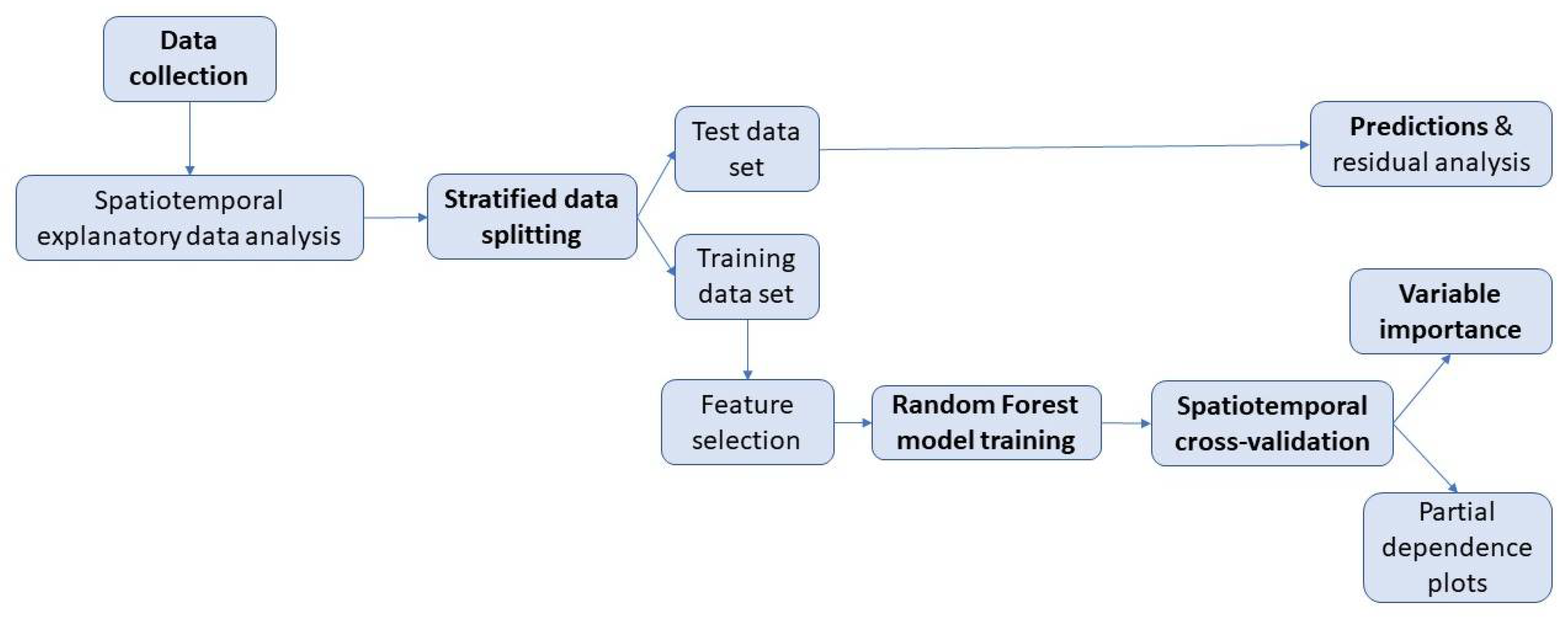
2.2. Analytical Framework

Figure 1 shows the research approach adopted in this study and depicts a detailed workflow and all the applied methodological approaches.

2.3. Data Collection

The data were collected from two sources: the Russian Federal State Statistics Service (RFSSS) and the Dairy Intelligence Agency (DIA, formerly the Russian Dairy Research Centre). The data were collected for 78 regions in the Russian Federation over a seven-year period (2013–2019). At the time of data collection, data for 2020 were not publicly available. The data were limited to seven years because the DIA only contains data from 2013 onwards. The aim of this research is to investigate the determinants of raw milk prices in Russia. Combining data before and after the introduction of embargo (2014) complicates the interpretation of results due to differences in the raw milk market. Thus, we kept the data for the period 2015–2019 (5 years). The collected data consist of 23 columns and 390 rows (8970 datapoints). The database includes the 78 Russian administrative regions (region name and region ID), the response variable (raw and log-transformed), and the 17 predictor variables for the period 2015–2019. Both response and predictor variables in the database show the annual values for the above-mentioned years. In the DIA database, only the annual values are provided.
The DIA collects annually statistical time series data on dairy science and contains information that is not currently offered by the RFSSS (“Population density”, “Total number of milk producers (companies)”, “Milk production per capita”, “Milk consumption per capita”, “Total need for milk”, “The total amount of processed milk”, “Total drinking milk production”, “Total cheese production”, “Total number of dairy companies”). In total, 78 regions were included, rather than the official number of 85 regions in the Russian Federation, as the DIA considers the following seven regions to be sub-regions of their larger neighbouring regions (Moscow city in the Moscow region, St. Petersburg in the Leningrad region, Sevastopol city in the Republic of Crimea, the Republic of Adygea in the Krasnodar region, the Khanti-Manssiskiy autonomous region and Jamalo-Nenetskij autonomous region in the Tyumen region, and the Nenetsk autonomous region in the Archangelsk region). However, the RFSSS separately provides data for these seven sub-regions. To match the data from the DIA, the RFSSS data from these seven regions were merged with the data for their larger neighbouring regions using the weighted average. All the data collected by RFSSS (“Gross regional product per capita”, “Population surplus”, “Livestock cattle”, “Investments in stock capital”, “Income per month per capita”, “Milk yield per cow”, “Milk price”) and was aggregated using population-weighted mean. A total of 17 potential explanatory variables were collected (Table 1).
Milk price (Euro/t) was provided by the RFSSS for the period 1999–2019. However, data before 2013 were not included in the analysis because the DIA does not contain data from before 2013. Finally, five years (2015–2019) were analysed, and the data for 2013 and 2014 were excluded to limit the effect of the introduced embargo. The descriptive statistics for all the collected variables are presented in Table A1.

2.4. Data Imputation

The resulting panel dataset contained 34 missing values in the explanatory variables (0.39%) and 6 missing values in the response variable (0.07%) in all years. These missing values were separately imputed with the available information for each region. Since the vast majority of explanatory variables did not show specific structural breaks, imputation based on median values was selected. However, the milk price showed an increasing linear trend over the years for the vast majority of regions. To maintain this trend, a linear interpolation was performed using the imputeTS package in R [18]. In the entire dataset, four regions included missing values in the response variable. For the linear interpolation the algorithm parameters were set as follows: time (start and end of the time series), frequency 1 (for one year step).

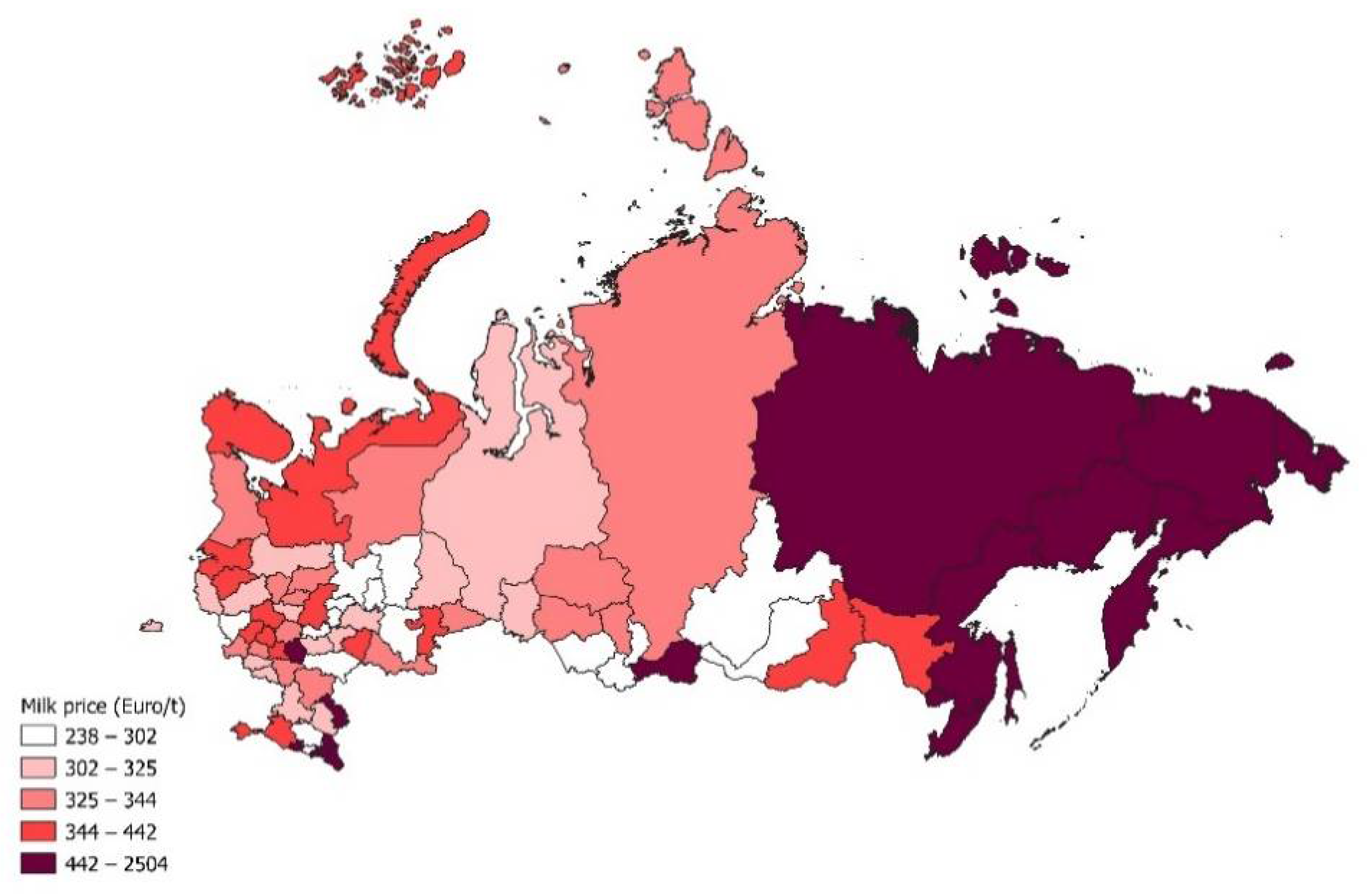
2.5. Spatial Analysis

Conventional spatial lag models [19] were performed at earlier stages of analysis, resulting in poor performance. Therefore, the RF model was used, due to the good predictive performance of ML models for data with non-linear relationships. The presence of spatial autocorrelation in the data was identified by separately calculating Moran’s I for spatial autocorrelation in milk prices for each studied year (2015–2019) in Russia. The value was the lowest in 2019 (0.451) and the highest in 2017 (0.627) and 2018 (0.621), while the remaining years (2015, 2016) showed a moderate level of spatial autocorrelation. Spatial analysis was undertaken in the form of Moran’s I, using GeoDa 1.18.0 (2020), and the spatial map was designed using QGIS 3.16.4—Hannover (QGIS Development Team (2020)).

2.6. Feature Selection

Prior to RF model training, the relevance of all 17 predictor variables for explaining the response variable was evaluated using the ‘all-relevant feature (variable) selection’ Boruta algorithm. The ‘all-relevant feature selection’ method aims to identify the relevance of explanatory variables to the response variable. This is an important step before ML modelling because it ensures that only relevant explanatory variables are used for model predictions. Thus, irrelevant and noisy predictors are not included in the analysis, maximising the model performance [20]. The Boruta algorithm was chosen from among the different relevant feature selection methods [20]. Recent studies show that Boruta has increased sensitivity and selective power in synthetic and real-world datasets, outperforming other common algorithms [21]. In short, the algorithm creates randomised copies of the explanatory variables (so-called “shadow variables”) by shuffling them. Subsequently, a relatively fast version of the random forest algorithm (“ranger random forest”) [22] is performed several times and the importance of each variable is calculated. Then, the variables that scored better than the maximum Z-score among all shadow variables are considered important, while the variables that scored lower are considered unimportant for the analysis [20].
Although all the variables were relevant for the explanation of milk price based on the Boruta algorithm, it was beneficial to exclude the collinear predictors because they may lead to the incorrect identification of significant predictors [23]. The presence of collinear variables in the prediction model can decrease explainability and create spurious associations between predictors and response variables [24]. Moreover, partial dependence plots (PDPs) assume the absence of multicollinearity among the variables [25].
Moreover, the collinear predictor variables were excluded from the dataset based on their relevance, which was derived from feature selection algorithm Boruta, as well as the correlation analysis. Subsequently, the correlation analysis, with a correlation coefficient threshold equal to 0.7, revealed collinear predictor variables, and those with the lower Boruta score were excluded.

2.7. Data Transformation

The explanatory data analysis showed that the milk price was highly right-skewed, and, thus, a log-transformation was applied. Normality is not a required assumption for RF [26]. However, recent studies have shown that, in case of severe skewness, the appropriate transformation can improve the prediction performance [27,28,29,30].

2.8. Random Forest

It should be noted that ML is a powerful data-driven method that develops very rapidly, and many new approaches for classification and regression problems are used, in parallel with traditional methods [31]. The success of the ML approach is determined by several factors, such as data quality and quantity (e.g., well-designed sampling schemes with sufficient and representative data for all examined sub-cases). Moreover, the exclusion of irrelevant, redundant, noisy or generally unreliable information used as predictors increases the model performance [32]. In addition, the ML data-driven models are empirically optimised, looking for the optimal solution [33]. Such models have been applied in various studies with agricultural data [10,11,12], as well as in dairy science [34,35,36,37]. To the authors’ knowledge, the determinants of producers’ milk prices in Russia have not previously been studied using ML algorithms. The motivation for using the RF model was that tree-based methods are good at capturing non-linear relationships in data and providing the variable importance [11]. Thus, the present study was one of the first attempts to examine the potential of ML as a quantitative tool in dairy science (e.g., dairy economics).
It is well known that RF is an ensemble ML method consisting of classification and regression trees [26]. In RF, the input training data are randomly, and with replacement, divided into several samples. Each of these samples is again sub-divided into two sub-samples (in-bag and out-of-bag sub-samples); then, the in-bag sub-sample is used to grow the tree. Thus, each tree is grown independently from the other trees and is not correlated with them, as a different random sample of observations and predictors are used. The different predictions from the trees are averaged to a final prediction in a regression problem. In the classification problem, the majority vote is used. In parallel, the prediction performance and variable importance are calculated based on the out-of-bag sample. The final model is applied to calculate the predictions in the test dataset [38].
Furthermore, RF has a good resistance to over-fitting [39] and a high predictive accuracy, even when many explanatory variables are used [40]. Over-fitting occurs when a trained model performs well on the training dataset, but has a poor predictive performance on the test (unseen) dataset, with the result that the difference between the prediction errors in the training dataset and the test dataset appears and continues to increase during model learning, apparently for reasons such as noise, hypothesis complexity, etc. [41].
The statistical analysis of the final dataset was performed with the R programming language [42]. Lastly, the ML algorithm RF model with spatiotemporal cross-validation was applied and its performance was compared with temporal and spatial cross-validation techniques using the Caret R Package [43] and Random Forest R Package [44].

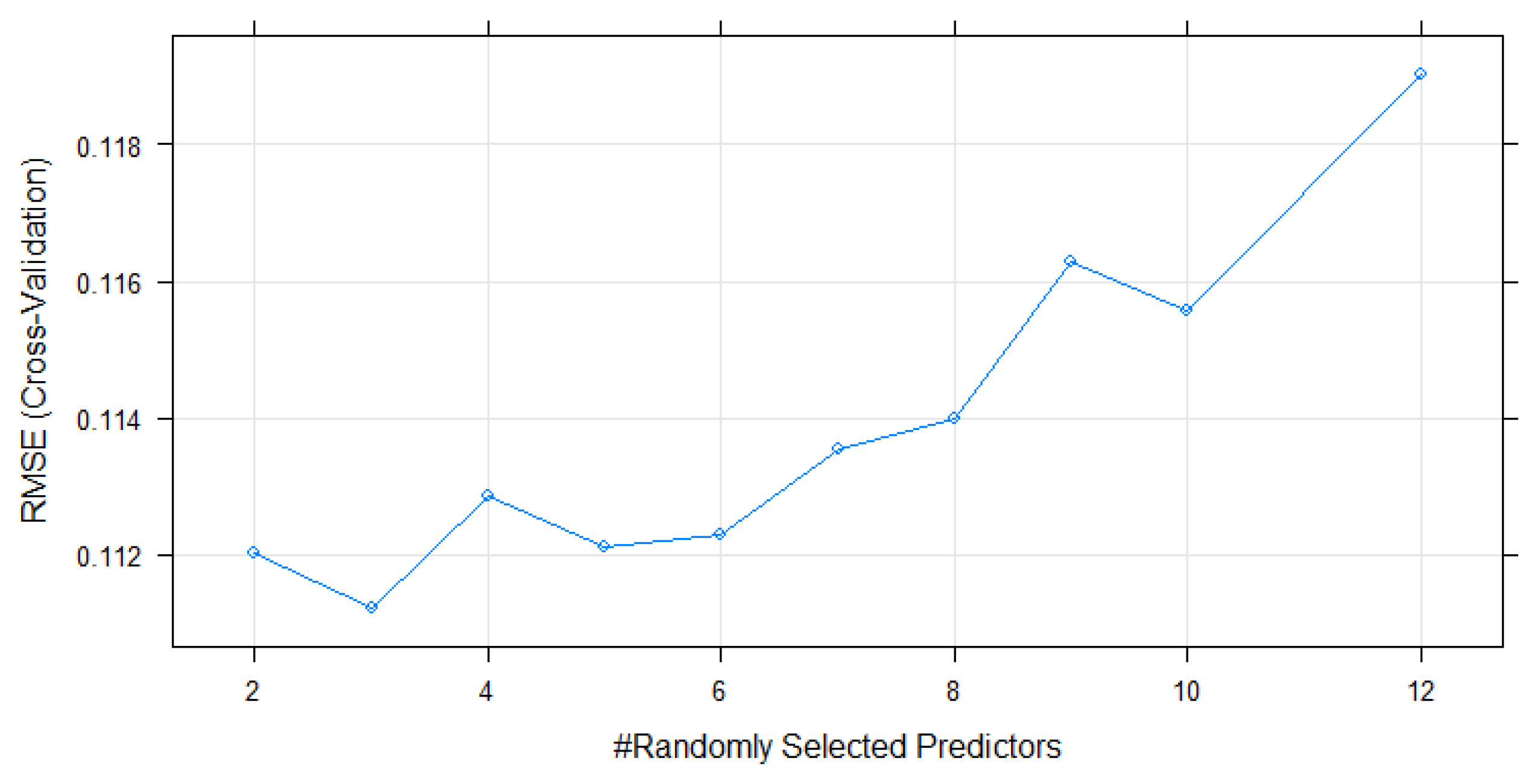
2.9. Model Training and Hyperparameter Optimisation

The splitting of data into training (80%) and test (20%) datasets was performed using stratified sampling on the temporal component (Year), resulting in a dataset with an equal number of observations per year. During the temporal and spatiotemporal cross-validation, the traditional time series splitting was applied, using some years to predict the remaining years. The explanatory data analysis showed a high heterogeneity among different administrative regions. The random forest is a data-driven method, and it is important to provide data that include the maximum available information (e.g., the entire univariate range of the response and predictor variables). Thus, we decided to keep all the regions in the training dataset, but not for all years.
The test dataset was kept out of the training and cross-validation and was only used for the final model assessment. Spatiotemporal cross-validation was applied to the dataset due to the temporal (Figure A1) and spatial autocorrelations (Figure 2, Table 2 revealed in the data.
Temporal cross-validation is a more appropriate method for time series data as the traditional random cross-validation does not account for the temporal structure of the data, leading to overoptimistic prediction errors [45,46].
The spatiotemporal cross-validation was performed using the CAST R package [47]. During the cross-validation phase, the training dataset was split five times based on the time component (Year). By doing this, one year was always kept out for validation. At the same time, a region (or a group of regions) was also kept out from training. The model was trained, and the validation was conducted for the remaining data. In the next split of the data, another year and another region (group of regions) were held out for prediction. Data loss related to the excluded year and excluded region (group of regions) occurred within the training dataset during the cross-validation phase. The procedure systematically repeated for all remaining years and regions. Spatiotemporal cross-validation represents a Leave-Location-and-Time-Out cross-validation technique that enables the proper implementation of spatiotemporal modelling [47].
The model predictions are made on the basis of excluded locations (regions) and excluded points of time (years), while random cross-validation leads to a biased prediction performance [48]. During temporal cross-validation, one year and all regions assigned with this year were excluded from the training and used for prediction, while in the spatial cross-validation, one region and all the years assigned to this region were excluded during every split of the data by rotation. Over-fitting by applying temporal and spatial cross-validation techniques can be identified through a comparison with random cross-validation [48].
In addition, RF is a relatively simple method because the most influential hyperparameter can be set according to the number of predictors that are available for splitting the data when growing a tree, known as the mtry parameter [49]. In total, nine different mtry values were tested and compared, based on the resultant Root Mean Square Error (RMSE), R-squared (R2) and Mean Absolute Error (MAE). The best tune of the model was chosen depending on minimal RMSE. The number of growing trees (ntree parameter) was kept constant at 500 trees, which is the default value [50]. Increasing the number of trees does not automatically improve the model’s performance [51]. The model was trained using the caret R package [43], which allows for hyperparameter optimisation as well as temporal, spatial and spatiotemporal cross-validation.
Lastly, the RF model with temporal, spatial and spatiotemporal cross-validation was performed in the present study, although, due to temporal and spatial autocorrelations of the data, the spatiotemporal cross-validation technique was chosen for the final model. The performances of three cross-validation techniques were compared and are presented in Table 3 (section “Results”). The final model was applied to the test dataset for an independent assessment of model performance in a new dataset, in which RMSE, MAE, R2 and residual characteristics were calculated.

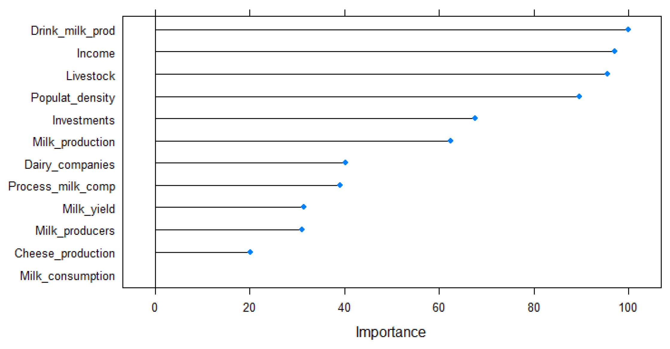
2.10. RF Variable Importance

RF calculates the variable importance of each predictor, based either on node impurity or permutation error. Node impurity (the number of times that each variable is chosen in each node in each tree of the ensemble) can be biased when the predictors vary in their scale or are correlated, and their sampling is performed with a replacement [52]. In contrast, importance (which is calculated by estimating the increase in the prediction error when shuffling the variable while simultaneously keeping all other variables unchanged) is more stable and unbiased [53,54]. Given the above-mentioned facts, the permutation importance for predictor variables was calculated in the present study. Finally, the PDPs for the eight most important variables were presented using the pdp package [55]. These plots visualise the partial dependence of the response variable on each single explanatory variable, with the aim of showing their relationship type [56].

3. Results

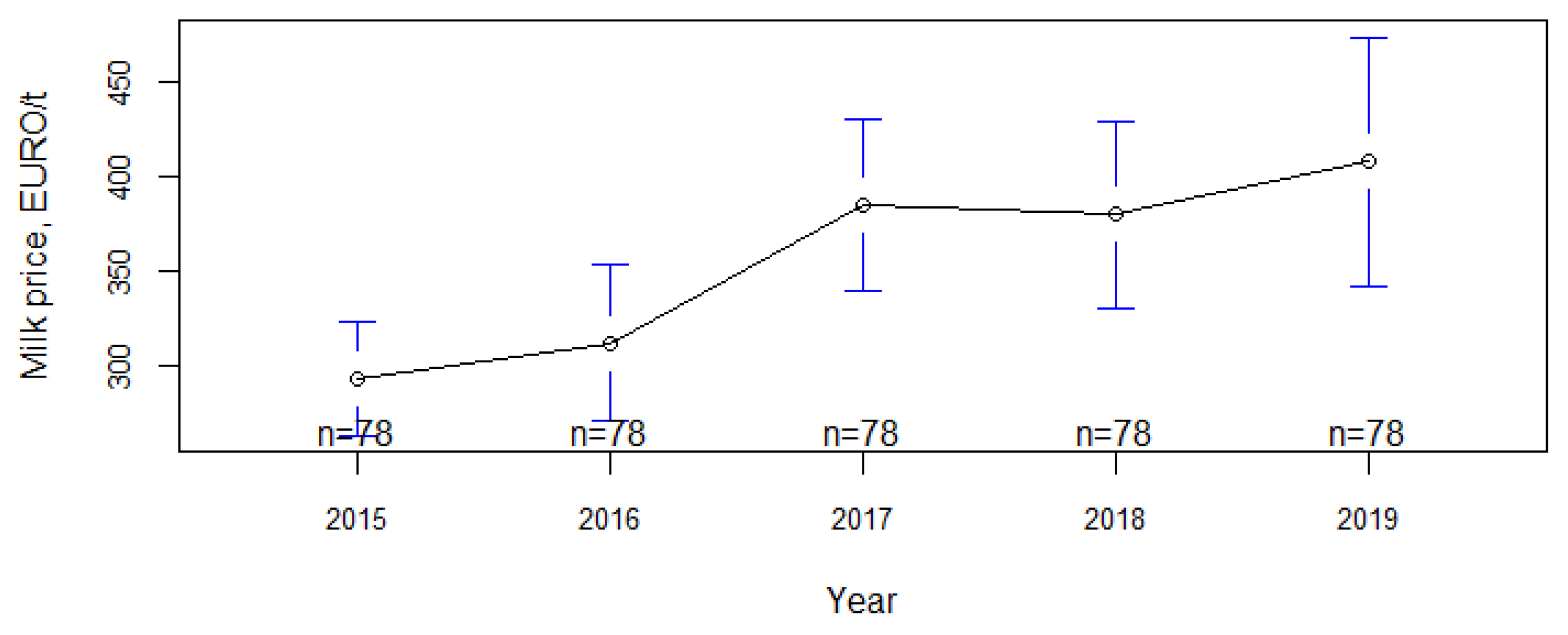
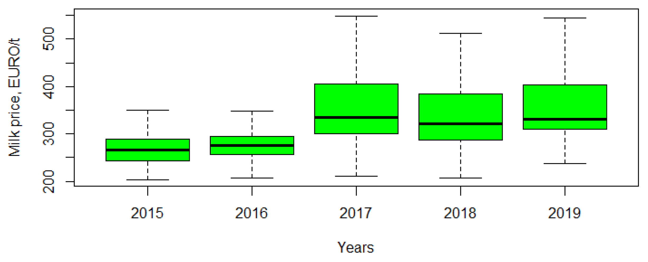
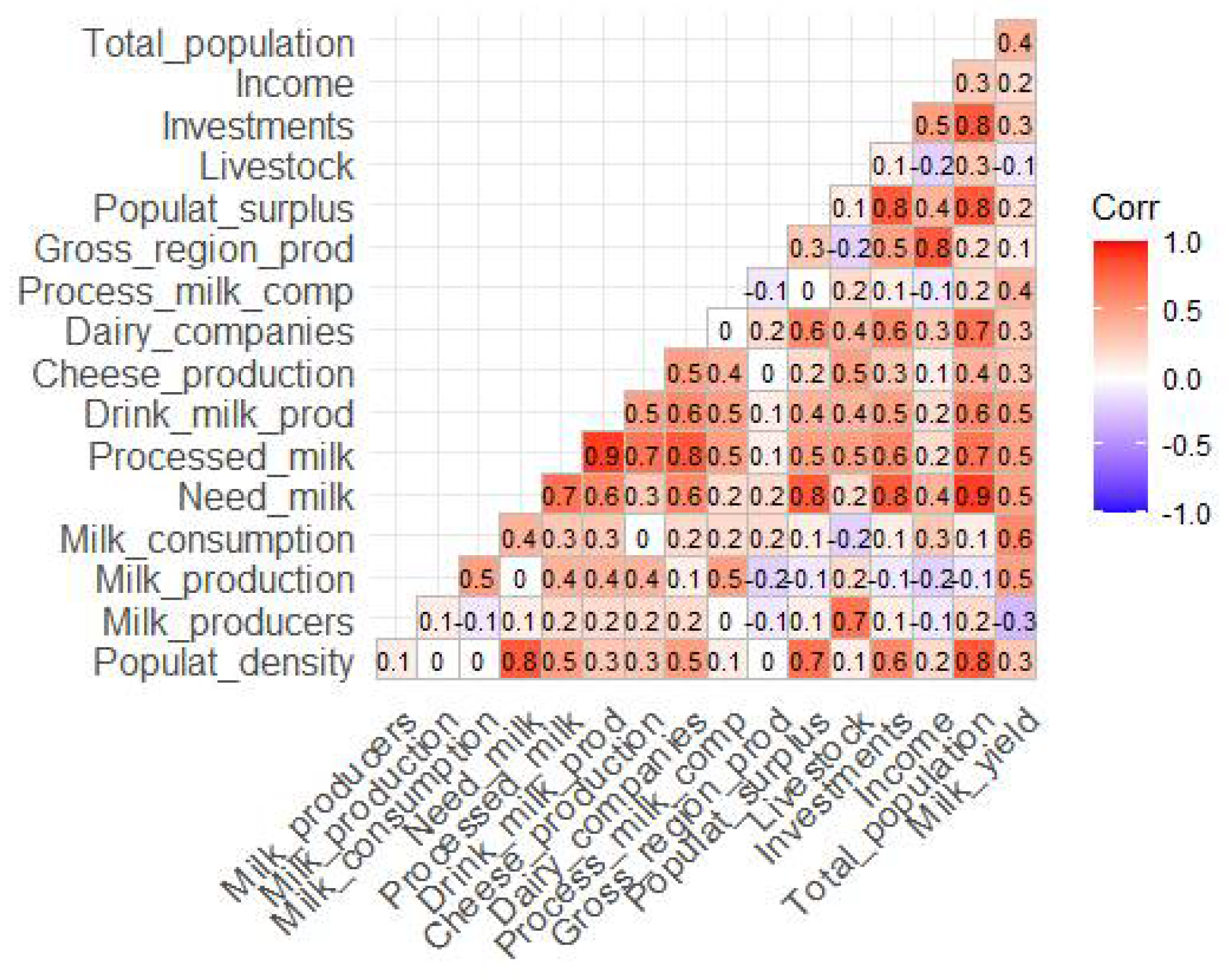
3.1. Exploratory Data Analysis

The analysis of the mean milk price in Russia showed a steady increase from 2015 to 2017, with a small drop in 2018 before the increase continued in 2019 (Figure 3).
The analysis of the period 2015–2019 showed that milk price rose in the period 2015–2017, then fell slightly in 2018 before continuing to rise again in 2019. A Kruskal–Wallis test confirmed that there was a statistically significant difference in milk prices between different years (p-value < 2.2 × 10⁻¹⁶). The range of the milk prices over the years 2015–2019 was 2348 Euros (from 156 Euro to 2504 Euros), while the mean milk price was 356 Euro/t. It should be noted that the range in milk prices in the last three years (2017–2019) was greater, showing a greater variance between the different regions (Figure A2). Furthermore, both median and mean prices were higher in those years.

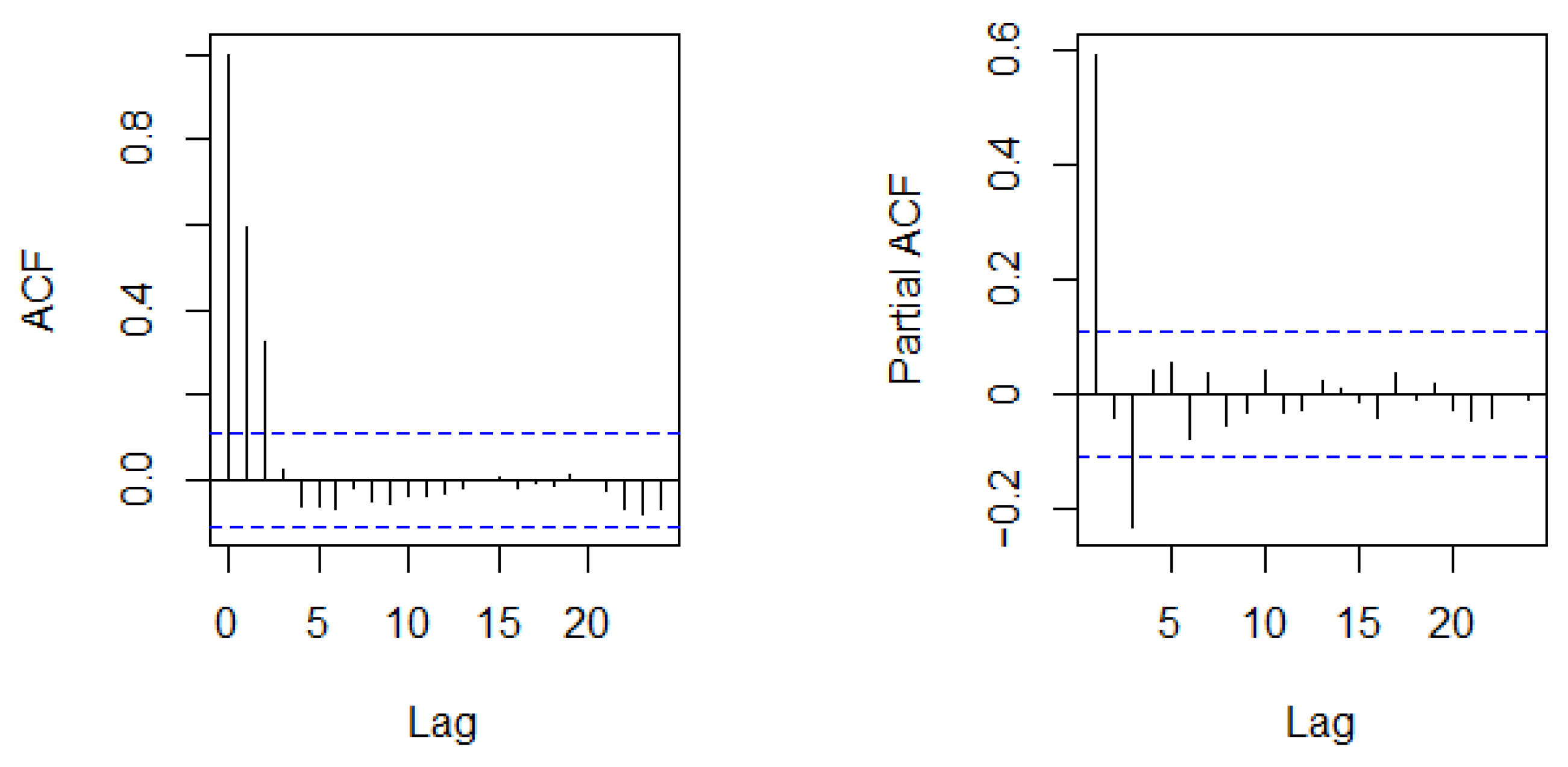
3.2. Spatial and Temporal Autocorrelation

A visualisation of milk prices in Russia in 2019 is given in Figure 2 (section “Materials and Methods”), which shows the spatial autocorrelation between regions. The northern regions had higher milk prices, while some southern regions of Russia generally demonstrated lower milk prices. From this map, it can be inferred that milk prices in some regions were affected by milk prices in neighbouring regions, representing a spatial autocorrelation. The data analysis showed that the raw milk price increased in almost all regions during the study period. Only the Irkutsk region and Stavropol region showed a decrease in raw milk prices, by 12% and 7%, respectively.
The spatial autocorrelation between regions was tested with Moran’s I, whose distribution over the years is presented in Table 2. The weights were created based on the Queen contiguity, with an order of contiguity equal to 1. The maximum number of neighbours in a region was nine, with the mean number of neighbours being equal to 4.54, while three regions without neighbours (Kaliningrad region, Republic of Crimea, Sakhalin region) were removed from the analysis. As a randomisation method, the 999 permutations method was applied.
The temporal autocorrelation between milk prices for the current year and for previous years was detected in data that were tested with the autocorrelation function (ACF) (Figure A1), where many years were located beyond the bounds that are significantly different from zero at the 5% level. Autocorrelation function (ACF) showed how the milk price in the current year was correlated with the milk price in the previous year and with the milk price in the year before that. Partial autocorrelation function showed the autocorrelation between milk prices, removing indirect correlations.

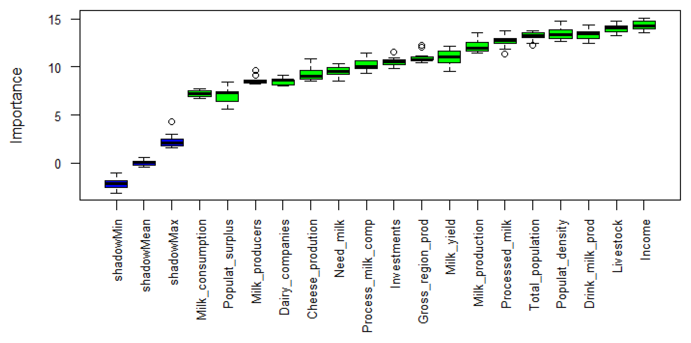
3.3. Results of the Feature Selection

Feature selection was conducted with the training dataset. The Boruta analysis showed that all 17 collected predictor variables were relevant to explaining the milk price (Figure 4). The majority of variables scored higher than the maximum shadow Z-score value among all shadow variables (blue boxplots), indicating potentially strong predictors (green boxplots). In Figure 4, ‘Importance’ is defined as the Z-score of each predictor variable, with the Z-score being calculated by dividing the average accuracy loss by its standard deviation [20]. Income showed the highest predictive ability, followed by livestock numbers, drinking milk production, population density and total population in the first five positions. However, several variables (milk consumption per capita, population surplus, etc.) had a relatively low importance. Nevertheless, the overall performance of these variables was higher than the maximum shadow Z-score, allowing for their inclusion in the final model. The Boruta algorithm showed that all the predictor variables were relevant for the explanation of milk price.
However, the correlation analysis revealed high correlation coefficients for several variables; hence, the threshold for excluding the collinear variables was set at 0.7 [23], and variables that scored higher than 0.7 (Figure A3) were excluded from analysis. At the same time, from a collinear pair of variables, a less relevant variable in the feature selection algorithm Boruta (Figure 4) was excluded from the subsequent analysis to increase the interpretability of the model. The following five predictor variables (out of all 17 collected predictor variables) were kept out of the analysis: gross regional product, total population, population surplus, need in milk and total amount of processed milk.

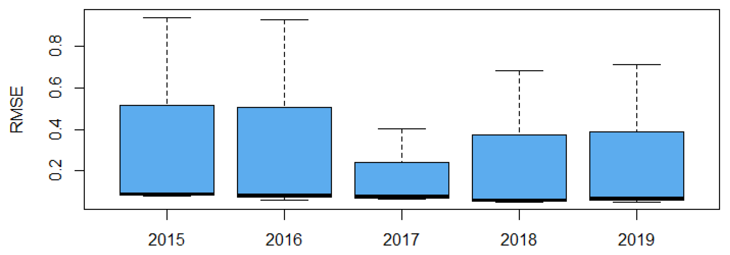
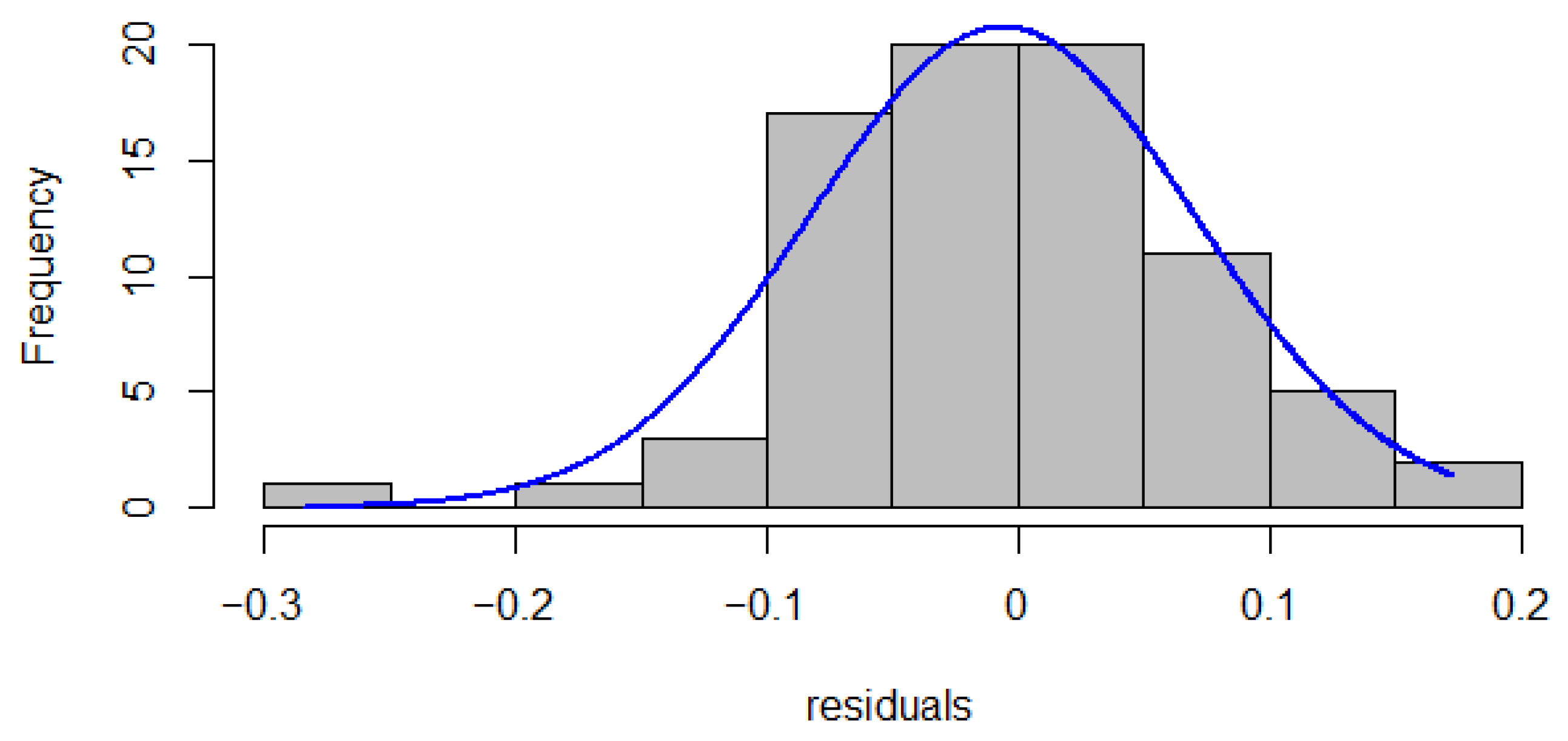
3.4. Results of RF Modelling

Due to temporal and spatial autocorrelations in the data, the spatiotemporal cross-validation technique was applied for a final model. During the optimisation process, the algorithm examined ten different mtry values, which are presented on the horizontal axis in Figure 5. The RMSE was minimal when mtry was 3. This value was close to the default value of mtry for regression (number of predictor variables divided by 3) in the random forest package [50]. The use of mtry values that were much higher or much lower than 3 increased the error, with the highest error being observed when mtry = 12 (Figure 5).
After the optimal mtry value was found, the final model was applied to the independent test dataset to evaluate its predictive ability. The analysis of the results showed good overall performance in the test dataset (Figure A4). This fact was also confirmed by low RMSE and MAE, as well as by its relatively high R2 (Table 3).
The predictive performance of the model was back-transformed into the initial scale (Euro). Additionally, partial dependence plots were created with the response variable in the initial scale (Euro). The different cross-validation technique assesses the model performance in a different way, without changing the model itself. At the end of each of three cross-validation circles, the model used the same amount of training data and captured the same relationships between response and predictor variables. This fact is confirmed by the similar performance of the test dataset. The results of the three different cross-validation strategies show that both the spatial and the temporal aspects of data play an important role in the raw milk prices.
Moreover, R2 in the test dataset was observed to be higher using the spatiotemporal cross-validation technique, while, in this case, the spatial and temporal structure of the data was considered. Due to spatiotemporal autocorrelations in the data, spatiotemporal cross-validation was a more appropriate technique.
The range of predicted values of the milk price was slightly smaller than the range of observed values. The maximum predicted value was underestimated, and the minimum predicted value was overestimated.
The good overall performance of the model was further shown by the residual characteristics. The range of residuals was relatively small, and the majority of them were distributed around zero and approximately normally distributed (Figure A5). The RMSE among the studied years was calculated (Figure A4). The range of prediction errors was higher in 2015 and 2016. Furthermore, in 2017 the range of prediction errors was slightly lower than the rest of the errors because the model could better predict the year 2017 due to the constant increasing trend of milk prices in previous years (2015 and 2016).

3.5. RF Model Interpretation

3.5.1. Variable Importance

Based on the RF variable importance, drinking milk production was the most important predictor, followed by income, livestock, population density, investments, milk production per capita and number of dairy companies (Figure 6).

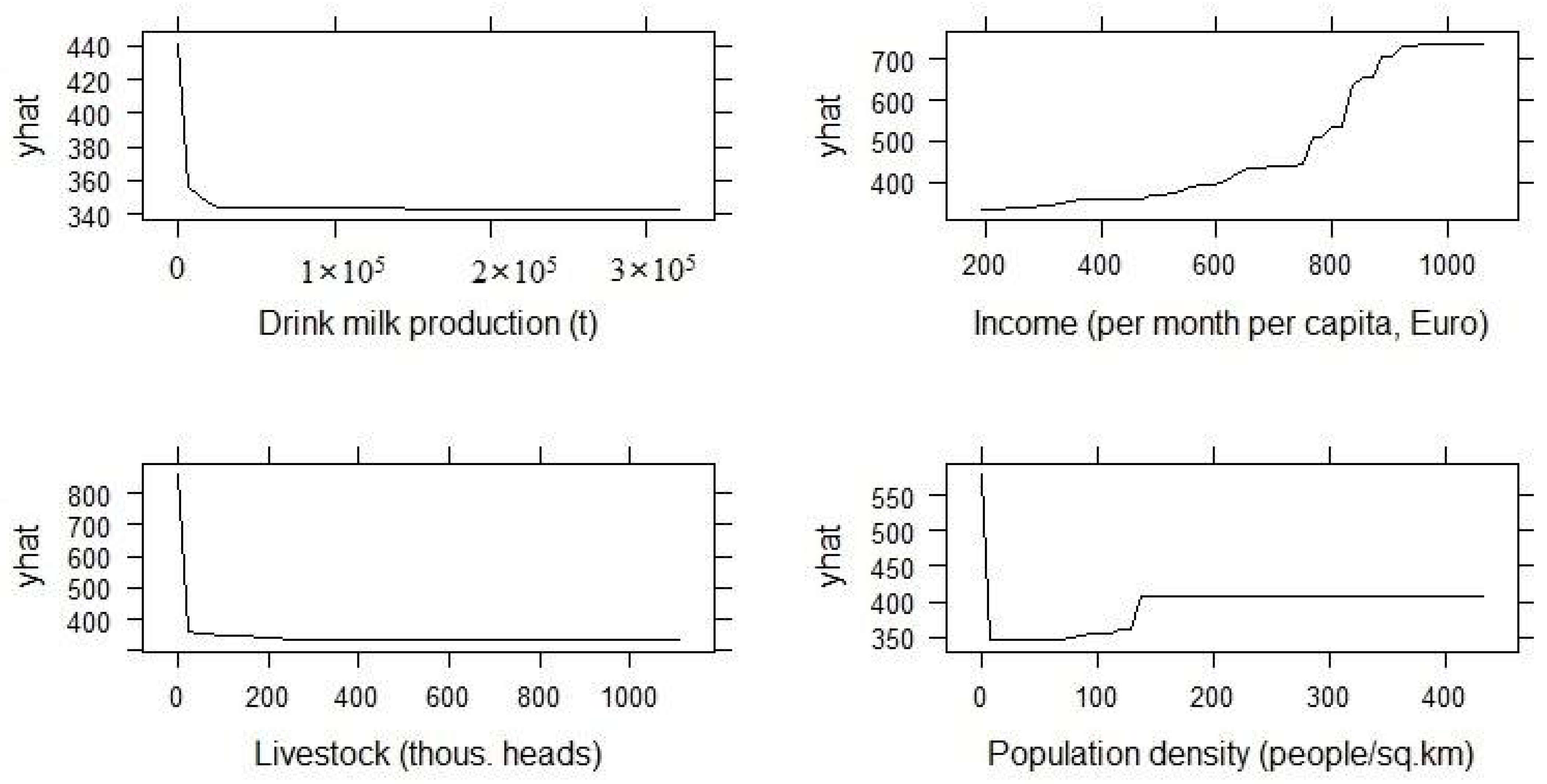
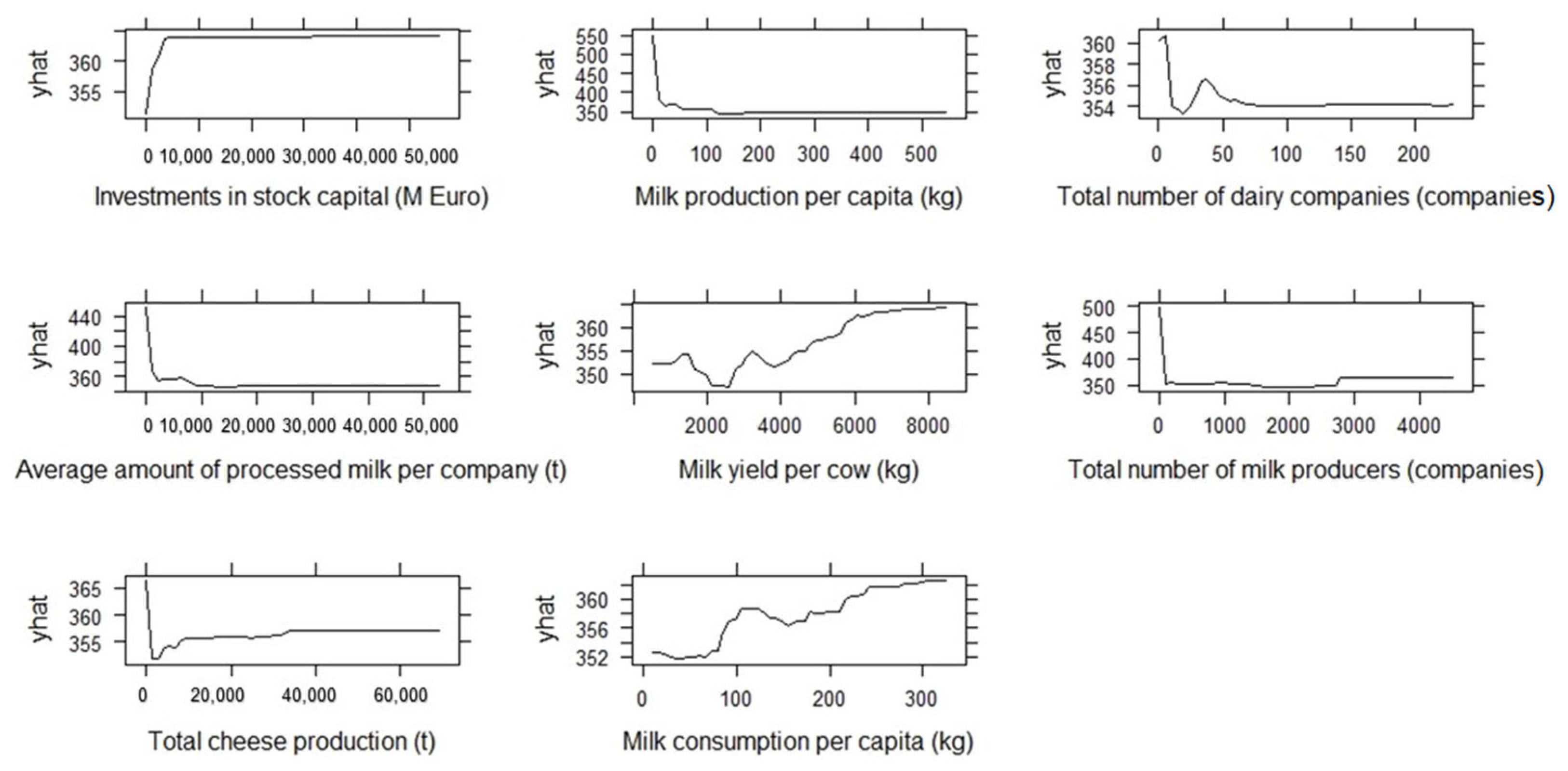
3.5.2. Partial Dependence Plots

Based on the analysis of PDPs (Figure 7) of the four most important variables, it was evident that drinking milk production had a clear monotonic relationship with milk price. More specifically, the rise in drinking milk production decreased the milk price. Nevertheless, the maximum increase occurred within the specific range of values (700–900 Euro/month), and then milk prices stabilised because the further income growth did not affect the milk prices.
The increase in income lead to a growth in milk prices. In contrast, the increase in livestock numbers decreased the milk price. It should be noted that in areas with extremely low livestock numbers (Chukotka autonomous region, Magadan region, etc.), an abrupt increase could be observed in milk price. The population density showed more complex patterns, similar to livestock monotonic trends. The PDPs for the next eight important predictor variables are presented in Figure A6.

4. Discussion

The present study analysed the determinants of milk price formation in Russia using the ML algorithm RF, which has a high predictive power and can detect which determinants are most important to the explanation of milk price. The feature selection algorithm Boruta and correlation analysis were used to exclude any irrelevant predictors from the model training. Although the results of the Boruta algorithm confirmed the relevance of the collected data, the exclusion of highly correlated predictors improved the interpretability of the results. The log transformation of the data was able to improve the predictive performance of the model further as it reduced the skewness of the milk price. Since ML modelling is a data-driven approach, the presence of a very few extreme observations reduced the model’s ability to learn these extreme cases. A spatiotemporal cross-validation technique was applied to consider the temporal and spatial structure of the data. It should be noted that the aim of this study was not to forecast milk prices, but to understand the main drivers influencing milk prices.
This study investigated milk price variability in Russian regions in the years from 2015 to 2019. The data analysis showed that the milk price continuously rose between 2015 and 2017, with a small drop in 2018, but the rise continued in 2019. This increase was probably due to the embargo, which forced Russia’s dairy sector to substitute imported dairy products with domestic production. Insufficient dairy production increased competition on the dairy market and consequently boosted the increase in milk prices in Russia [4]. Generally, an increase in milk price might be considered a positive development because farmers and milk producers receive higher prices for raw milk. However, the supply of high-quality raw milk is a serious problem in Russia due to the lack and low quality of feeding resources and hygiene [4], as well as the contamination of raw milk with antibiotics [57].
In 2014, the global political conflict involving Ukraine (Crimea) resulted in sanctions being imposed on the Russian Federation, which responded by introducing an embargo on the imports of agricultural and food products (including milk and dairy products) from the European Union, Norway, Australia, the United States of America and Canada [58]. However, it would appear that the embargo had no major negative effect on the consumption level in Russia, because Russian consumers adapted their buying behaviour to the new situation and started consuming a larger proportion of Russian products [59]. In this respect, studies have shown that milk price changes in Russia are affected by innovations and investment in the Russian dairy sector in a way that is independent of the international dairy markets [60].
The highest milk prices were observed in the Chukotka autonomous district, Magadan region and Kamchatka territory (source: RFSSS). All these regions are located in the far east of Russia, where there are scarce feeding resources, an extremely cold climate, few milk producers, livestock and dairy companies, and a low population density (as can be seen from the data collected from RFSSS and DIA). Moreover, in many of these regions, there is a poorly developed infrastructure that should be further improved [61].
The RF variable importance showed that drinking milk production was the most important determinant of raw milk prices in Russia. The increase in drinking milk production leads to decreases in milk prices, which can be explained by the market being overfilled with drinking milk, which decreases the price of drinking milk. This development forces raw milk prices to fall accordingly. Consequently, the more drinking milk the region produces, the lower the raw milk prices in this region.
Income was second the most important factor in determining the changes and fluctuations in milk prices in Russian regions. Increasing average per capita income contributes to improvements in livelihood, development of the region and a growth in demand and consumers’ willingness to pay, and also generates additional purchasing power, etc. The increasing purchasing power of the population will create an attractive climate for developing the dairy industry in the region, which will constantly affect the raw milk price. This attracts new investments to the region and increases the price of consumer goods, particularly dairy products. Higher consumer prices for dairy products could be a reason for the higher producer prices for raw milk in the region. Dairy companies can make a greater profit and are able to pay milk producers more for raw milk. Increasing income in the region leads to a rise in milk price.
Furthermore, livestock numbers were also one of the most important variables for the explanation of milk price in Russia. The more livestock a region has, the greater the milk supply and the larger the total amount of raw milk in the region. Thus, milk prices will decrease due to the rise in the provision of raw milk. Dairy companies will then have a larger raw milk supply and more options to procure raw milk. Therefore, livestock directly influences the milk price. For example, in most northern and far-eastern Russian regions, the number of milk producers is low and is combined with high raw milk prices. More milk producers or larger dairy farms could lead to an increase in livestock in the region. Therefore, a rise in livestock numbers leads to a fall in raw milk price.
Moreover, population density was also one of the most important predictor variables influencing raw milk prices in Russia. In the extremely low populated regions, raw milk prices are higher than in other regions. In the regions with a medium population density, the milk prices increase. However, in the highly populated regions, raw milk prices remain stable. Thus, the population density shows a complex relationship with milk prices and seems to not have any monotonic trend. This phenomenon can be explained through the non-linear relationship between population density and milk prices in Russia in the studied period (2015–2019).
The limitation of this study is that administrative regions had to be used as an approximation of spatial heterogeneity. However, some regions are very large, and whether the prices for these regions would can represent the entire region in the same way remains unclear. DIA was founded in 2013, providing important data for the dairy sector. Unfortunately, data for the years before 2013 are not provided by RFSSS database. This limits the ability to study the milk market before 2013. Additionally, DIA only provides data on an annual scale and does not allow for a study of the seasonal variations in the raw milk prices. Moreover, both databases do not provide data for the higher administrative levels (e.g., districts of each region). Consequently, the spatial heterogeneity inside each region is shadowed (e.g., differences between urban and rural areas). The different size and shape of each region results in an uneven number of assigned neighbours in the spatial analysis.
Among the different examined methods, the Queen continuity offers the most realistic representation of the spatial relationships among Russian regions. Nevertheless, the three regions (Republic of Crimea, Kaliningrad region, and Sakhalin region) became isolates, as they did not share any common borders with other neighbour regions. These three regions were excluded from the calculation of the Moran’s I, but not from the random forest modelling.
The potential of ML approaches in agriculture is continuously growing because they provide an efficient way of processing data with complex (non-linear) relationships. Future research could include the study of other potential covariates such as transportation costs, fodder costs, infrastructure development, and age structure of the population, assuming that this information will be publicly available at a later stage. In addition, the study of other machine learning methods (artificial neural networks, support vector machines, etc.) could further enhance the understanding of milk markets in Russia. We would like to investigate the milk prices using finer scale data in both space and time, i.e., the sub-regions inside each region, and based on monthly data.

5. Conclusions

Raw milk prices increased in almost all Russian regions in the period 2015–2019. As expected, the regional raw milk prices exhibited spatial and temporal autocorrelations. However, the consideration of spatial and temporal autocorrelations in the dataset and the application of spatiotemporal cross-validation led to a decrease in the predictive performance of the RF in the training dataset compared with the use of temporal cross-validation techniques. Thus, spatiotemporal cross-validation was applied before RF model training. Regarding the determinants of regional milk price, the ML algorithm RF was used to estimate their influence on the response variable in the dataset. The results showed that drinking milk production, income, livestock numbers and population density were the four most important determinants (of those used in this study) when explaining the regional raw milk price in Russia. An increase in drinking milk production and livestock numbers in a region led to a decrease in raw milk price, but an increase in the income led to an increase in milk price. The relationship between milk prices and population density was non-linear. The findings of the present study could contribute to the stakeholders’ decision-making processes in the dairy supply chain in Russia, especially milk producers and dairy companies.

Author Contributions

The authors of this paper contributed as follows: Conceptualization, S.K. and S.H.; methodology, S.K.; software, S.K.; validation, S.K.; formal analysis, S.K.; investigation, S.K.; resources, S.H.; data curation, S.K.; writing—original draft preparation, S.K.; writing—review and editing, S.H.; visualization, S.K.; supervision, S.H.; project administration, S.H. All authors have read and agreed to the published version of the manuscript.

Funding

This research received no external funding.

Institutional Review Board Statement

Not applicable.

Data Availability Statement

The dataset and scripts generated for this study are available upon reasonable request to the corresponding author.

Acknowledgments

The authors thank the anonymous reviewers and the editor, as well as Professor Loy and members of the Department of Agricultural Economics in Kiel for valuable comments on earlier versions of the manuscript.

Conflicts of Interest

The authors declare no conflict of interest.

Appendix A

Figure A1. Autocorrelation function (ACF) and partial autocorrelation function (PACF) for milk price.
Agriculture 12 01006 g0a1
Figure A2. Boxplots for milk prices without outliers (2015–2019).
Agriculture 12 01006 g0a2
Figure A3. Correlation plot for all 17 collected explanatory variables Red color in the correlation plot indicates the correlation coefficients greater than zero; blue color indicates the correlation coefficients smaller than zero).
Agriculture 12 01006 g0a3
Figure A4. Prediction root mean square errors (RMSE) for different years in the test dataset.
Agriculture 12 01006 g0a4
Figure A5. Histogram of residuals distribution.
Agriculture 12 01006 g0a5
Figure A6. Partial dependence plots (PDPs) for the next eight important predictor variables: investments, milk production, number of dairy companies, amount of processed milk per company, milk yield, number of milk producers, cheese productions and milk consumption.
Agriculture 12 01006 g0a6
Table A1. Descriptive statistics of the collected dataset.
VariablenMinPctile (25)MedianPctile (75)MaxMeanSD
Milk_price390155.8271.3304.3354.12503.7356.1215.1
Log_milk_price3902.22.42.52.63.42.50.1
Populat_density3900.15.223.342.4432.833.952.2
Milk_producers3901151.2253.54734506393.3481.2
Milk_production3900.255.198.95170.2542.6132.1108.4
Milk_consumption39010.186.3144.0193.0324142.467.4
Need_milk390381182,008.2165,124.5278,7003,975,390287,775.4490,548.1
Processed_milk390141,225135,650294,6501,830,000234,591.4290,050
Drink_milk_prod3900.39711.340,621.6107,963.8321,112.270,532.976,357.4
Cheese_production3900116.5857.34470.268,971.15300.910,872.7
Dairy_companies390112233422930.333.6
Process_milk_comp39011953.26129.510,471.152,692.37794.57434.2
Gross_region_prod3901362.83304.84462.26142.630,680.65673.74405.5
Populat_surplus390−22,135−7356.5−3576960.5154,016−137.117,253.0
Livestock390089.8169.3290.31110.9234.6220.3
Investments390116.4641.31284.62546.955,544.72671.95498.4
Income390190.6289.3325.1386.31062.4357.8126.5
Total_population39049,505796,878.81,192,8432,405,15620,291,9341,880,8212,444,763
Milk_yield3905153823.54584.55532.284624550.31518.7

References

  1. Wegren, S.K.; Elvestad, C. Russia’s food self-sufficiency and food security: An assessment. Post-Communist Econ. 2018, 30, 565–587. [Google Scholar] [CrossRef]
  2. Solodukha, P.V.; Maiorova, E.A.; Shinkareva, O.V. Social and economic consequences of influence of food embargo on production of milk and dairy products in Russia. Ecol. Agric. Sustain. Dev. 2019, 2019, 297–305. [Google Scholar]
  3. Decree of the President of the Russian Federation of 21 January 2020 N 20. On approval of the Doctrine of Food Security of the Russian Federation. Available online: http://ivo.garant.ru/#/document/73438425/paragraph/1/doclist/34006/showentries/0/highlight/%D0%A3%D0%BA%D0%B0%D0%B7%20%D0%9F%D1%80%D0%B5%D0%B7%D0%B8%D0%B4%D0%B5%D0%BD%D1%82%D0%B0%20%D0%A0%D0%A4%2021.01.2020:3 (accessed on 15 September 2021).
  4. Nosov, V.V.; Suray, N.M.; Mamaev, O.A.; Chemisenko, O.V.; Panov, P.A.; Pokidov, M.G. Milk production dynamics in the Russian Federation: Causes and consequences. IOP Conf. Ser Earth Environ. Sci. 2020, 548, 022091. [Google Scholar] [CrossRef]
  5. Kulikov, I.M.; Minakov, I.A. Food security: Problems and prospects in Russia. Sci. Pap. Ser. Manag. Econ. Eng. Agric. Rural. Dev. 2019, 19, 141–147. [Google Scholar]
  6. Wegren, S.K. The Russian food embargo and food security: Can household production fill the void? Eurasian Geogr. Econ. 2014, 55, 491–513. [Google Scholar] [CrossRef]
  7. Guziy, S. The market of milk and dairy products in Russia: Peculiarities, tendencies and prospects of development. In The Agri-Food Value Chain: Challenges for Natural Resources Management and Society; Slovak University of Agriculture: Nitra, Slovakia, 2016; pp. 770–776. [Google Scholar]
  8. Artemova, E.I.; Kremyanskaya, E.V. Determinants of the development of the domestic milk market in the context of import substitution. Polythem. Netw. Electron. Sc. J. Kuban State Agrar. Univ. 2016, 116, 882–896. [Google Scholar]
  9. McQueen, R.J.; Garner, S.R.; Nevill-Manning, C.G.; Witten, I.H. Applying machine learning to agricultural data. Comput. Electron. Agric. 1995, 12, 275–293. [Google Scholar] [CrossRef] [Green Version]
  10. Balducci, F.; Impedovo, D.; Pirlo, G. Machine learning applications on agricultural datasets for smart farm enhancement. Machines 2018, 6, 38. [Google Scholar] [CrossRef] [Green Version]
  11. Storm, H.; Baylis, K.; Heckelei, T. Machine learning in agricultural and applied economics. Eur. Rev. Agric. Econ. 2020, 47, 849–892. [Google Scholar] [CrossRef]
  12. Saltzman, B.; Yung, J. A machine learning approach to identifying different types of uncertainty. Econ. Lett. 2018, 171, 58–62. [Google Scholar] [CrossRef]
  13. Hong, D.; Gao, L.; Yao, J.; Zhang, B.; Plaza, A.; Chanussot, J. Graph convolutional networks for hyperspectral image classification. IEEE Trans. Geosci. Remote Sens. 2020, 59, 5966–5978. [Google Scholar] [CrossRef]
  14. Han, J.; Zhang, D.; Cheng, G.; Liu, N.; Xu, D. Advanced deep-learning techniques for salient and category-specific object detection: A survey. IEEE Signal Process. Mag. 2018, 35, 84–100. [Google Scholar] [CrossRef]
  15. Guo, C.; Cui, Y. Machine learning exhibited excellent advantages in the performance simulation and prediction of free water surface constructed wetlands. J. Environ. Manag. 2022, 309, 114694. [Google Scholar] [CrossRef]
  16. Dahiya, N.; Gupta, S.; Singh, S.A. Review Paper on Machine Learning Applications, Advantages, and Techniques. ECS Trans. 2022, 107, 6137. [Google Scholar] [CrossRef]
  17. Goodwin, B.K. Multivariate cointegration tests and the law of one price in international wheat markets. Appl. Econ. Perspect. Policy 1992, 14, 117–124. [Google Scholar] [CrossRef]
  18. Moritz, S.; Bartz-Beielstein, T. ImputeTS: Time Series Missing Value Imputation in R. R J. 2017, 9, 207–218. [Google Scholar] [CrossRef] [Green Version]
  19. Anselin, L. Spatial Econometrics: Methods and Models; Springer: Dordrecht, The Netherlands, 1988. [Google Scholar] [CrossRef] [Green Version]
  20. Kursa, M.B.; Rudnicki, W.R. Feature selection with the Boruta package. J. Stat. Softw. 2010, 36, 1–13. [Google Scholar] [CrossRef] [Green Version]
  21. Degenhardt, F.; Seifert, S.; Szymczak, S. Evaluation of variable selection methods for random forests and omics data sets. Briefings Bioinf. 2019, 20, 492–503. [Google Scholar] [CrossRef] [Green Version]
  22. Wright, M.N.; Wager, S.; Probst, P. Package “ranger”: A Fast Implementation of Random Forests (Version 0.13.1) [R Package]. 2021. Available online: https://cran.r-project.org/web/packages/ranger/ranger.pdf (accessed on 15 September 2021).
  23. Dormann, C.F.; Elith, J.; Bacher, S.; Buchmann, C.; Carl, G.; Carré, G.; Marquéz, J.R.G.; Gruber, B.; Lafourcade, B.; Leitão, P.J.; et al. Collinearity: A review of methods to deal with it and a simulation study evaluating their performance. Ecography 2013, 36, 27–46. [Google Scholar] [CrossRef]
  24. Leeuwenberg, A.M.; van Smeden, M.; Langendijk, J.A.; van der Schaaf, A.; Mauer, M.E.; Moons, K.G.; Reitsma, J.B.; Schuit, E. Comparing methods addressing multi-collinearity when developing prediction models. arXiv 2021, arXiv:210101603. [Google Scholar] [CrossRef]
  25. Molnar, C. Interpretable Machine Learning: A Guide for Making Black Box Models Explainable. 2021. Available online: https://christophm.github.io/interpretable-ml-book/index.html (accessed on 15 September 2021).
  26. Breiman, L. Random forests. Mach. Learn. 2001, 45, 5–32. [Google Scholar] [CrossRef] [Green Version]
  27. Jiang, Y.; Cukic, B.; Menzies, T. Can data transformation help in the detection of fault-prone modules? In DEFECTS’ 08: Proceedings of the 2008 Workshop on Defects in Large Software Systems; Association for Computing Machinery: New York, NY, USA, 2008; pp. 16–20. [Google Scholar] [CrossRef] [Green Version]
  28. Lütkepohl, H.; Xu, F. The role of the log transformation in forecasting economic variables. Empir. Econ. 2012, 42, 619–638. [Google Scholar] [CrossRef] [Green Version]
  29. Stevens, F.R.; Gaughan, A.E.; Linard, C.; Tatem, A.J. Disaggregating census data for population mapping using random forests with remotely-sensed and ancillary data. PLoS ONE 2015, 10, e0107042. [Google Scholar] [CrossRef] [Green Version]
  30. Curran-Everett, D. Explorations in statistics: The log transformation. Adv. Physiol. Educ. 2018, 42, 343–347. [Google Scholar] [CrossRef] [PubMed]
  31. Trawinski, B.; Smętek, M.; Telec, Z.; Lasota, T. Nonparametric statistical analysis for multiple comparison of machine learning regression algorithms. Int. J. Appl. Math. Comput. Sci. 2012, 22, 867–881. [Google Scholar] [CrossRef]
  32. Hall, M.A. Correlation-based feature selection of discrete and numeric class machine learning. In Computer Science Working Papers (Working Paper 00/08); University of Waikato, Department of Computer Science: Hamilton, New Zealand, 2000. [Google Scholar]
  33. Goldstein, B.A.; Navar, A.M.; Carter, R.E. Moving beyond regression techniques in cardiovascular risk prediction: Applying machine learning to address analytic challenges. Eur. Heart J. 2017, 38, 1805–1814. [Google Scholar] [CrossRef] [PubMed] [Green Version]
  34. Shahinfar, S.; Page, D.; Guenther, J.; Cabrera, V.; Fricke, P.; Weigel, K. Prediction of insemination outcomes in Holstein dairy cattle using alternative machine learning algorithms. J. Dairy Sci. 2014, 97, 731–742. [Google Scholar] [CrossRef] [PubMed] [Green Version]
  35. Borchers, M.R.; Chang, Y.M.; Proudfoot, K.L.; Wadsworth, B.A.; Stone, A.E.; Bewley, J.M. Machine-learning-based calving prediction from activity, lying, and ruminating behaviors in dairy cattle. J. Dairy Sci. 2017, 100, 5664–5674. [Google Scholar] [CrossRef]
  36. Ma, W.; Fan, J.; Li, Q.; Tang, Y. A raw milk service platform using BP Neural Network and Fuzzy Inference. Inf. Process. Agric. 2018, 5, 308–319. [Google Scholar] [CrossRef]
  37. Volkmann, N.; Kulig, B.; Hoppe, S.; Stracke, J.; Hensel, O.; Kemper, N. On-farm detection of claw lesions in dairy cows based on acoustic analyses and machine learning. J. Dairy Sci. 2021, 104, 5921–5931. [Google Scholar] [CrossRef]
  38. Mota, L.F.; Pegolo, S.; Baba, T.; Peñagaricano, F.; Morota, G.; Bittante, G.; Cecchinato, A. Evaluating the performance of machine learning methods and variable selection methods for predicting difficult-to-measure traits in Holstein dairy cattle using milk infrared spectral data. J. Dairy Sci. 2021, 104, 8107–8121. [Google Scholar] [CrossRef]
  39. Cutler, D.R.; Edwards, T.C., Jr.; Beard, K.H.; Cutler, A.; Hess, K.T.; Gibson, J.; Lawler, J.J. Random forests for classification in ecology. Ecology 2007, 88, 2783–2792. [Google Scholar] [CrossRef]
  40. Svetnik, V.; Liaw, A.; Tong, C.; Culberson, J.C.; Sheridan, R.P.; Feuston, B.P. Random forest: A classification and regression tool for compound classification and QSAR modeling. J. Chem. Inf. Comput. Sci. 2003, 43, 1947–1958. [Google Scholar] [CrossRef]
  41. Ying, X. An overview of overfitting and its solutions. J. Phys. Conf. Ser. 2019, 1168, 022022. [Google Scholar] [CrossRef]
  42. R Core Team. R: A Language and Environment for Statistical Computing. (Version 4.0.4) [Computer Software]; R Foundation for Statistical Computing: Vienna, Austria, 2021; Available online: https://www.R-project.org/ (accessed on 7 September 2021).
  43. Kuhn, M.; Wing, J.; Weston, S.; Williams, A.; Keefer, C.; Engelhardt, A.; Cooper, T.; Mayer, Z.; Kenkel, B. Caret: Classification and Regression Training. [R Package] (Version 6.0-86). 2022. Available online: https://cran.r-project.org/web/packages/caret/caret.pdf (accessed on 15 September 2021).
  44. Liaw, A. Randomforest: Breiman and Cutler’s Random Forests for Classification and Regression. [R Package] (Version 4.7–1.1). Available online: https://cran.r-project.org/web/packages/randomForest/randomForest.pdf (accessed on 15 September 2021).
  45. Roberts, D.R.; Bahn, V.; Ciuti, S.; Boyce, M.S.; Elith, J.; Guillera-Arroita, G.; Hauenstein, S.; Lahoz-Monfort, J.J.; Schröder, B.; Thuiller, W.; et al. Cross-validation strategies for data with temporal, spatial, hierarchical, or phylogenetic structure. Ecography 2017, 40, 913–929. [Google Scholar] [CrossRef]
  46. Wang, Q.; Bovenhuis, H. Validation strategy can result in an overoptimistic view of the ability of milk infrared spectra to predict methane emission of dairy cattle. J. Dairy Sci. 2019, 102, 6288–6295. [Google Scholar] [CrossRef]
  47. Meyer, H.; Reudenbach, C.; Ludwig, M.; Nauss, T.; Pebesma, E. CAST: “Caret” Applications for Spatial-Temporal Models (Version 0.5.1) [R Package]. Available online: https://cran.r-project.org/web/packages/CAST/CAST.pdf (accessed on 16 September 2021).
  48. Meyer, H.; Reudenbach, C.; Hengl, T.; Katurji, M.; Nauss, T. Improving performance of spatio-temporal machine learning models using forward feature selection and target-oriented validation. Environ. Model. Softw. 2018, 101, 1–9. [Google Scholar] [CrossRef]
  49. Probst, P.; Wright, M.N.; Boulesteix, A.L. Hyperparameters and tuning strategies for random forest. WIREs Data Min. Knowl. Discovery 2019, 9, e1301. [Google Scholar] [CrossRef] [Green Version]
  50. Liaw, A.; Wiener, M. Classification and regression by randomForest. R News 2002, 2, 18–22. [Google Scholar]
  51. Oshiro, T.M.; Perez, P.S.; Baranauskas, J.A. How many trees in a random forest? In Machine Learning and Data Mining in Pattern Recognition; Perner, P., Ed.; Springer: Berlin/Heidelberg, Germany, 2012; pp. 154–168. [Google Scholar] [CrossRef]
  52. Kuhn, M. Building predictive models in R using the caret package. J. Stat. Softw. 2008, 28, 1–26. [Google Scholar] [CrossRef] [Green Version]
  53. Strobl, C.; Boulesteix, A.L.; Zeileis, A.; Hothorn, T. Bias in random forest variable importance measures: Illustrations, sources and a solution. BMC Bioinf. 2007, 8, 25. [Google Scholar] [CrossRef] [PubMed] [Green Version]
  54. Strobl, C.; Boulesteix, A.L.; Kneib, T.; Augustin, T.; Zeileis, A. Conditional variable importance for random forests. BMC Bioinf. 2008, 9, 307. [Google Scholar] [CrossRef] [PubMed] [Green Version]
  55. Greenwell, B. Package “pdp”: Partial Dependence Plots (Version 0.6.0) [R Package]. 20 July 2017. Available online: https://mran.microsoft.com/snapshot/2018-06-07/web/packages/pdp/pdp.pdf (accessed on 15 September 2021).
  56. Greenwell, B. pdp: An R Package for Constructing Partial Dependence Plots. R J. 2017, 9, 421–436. [Google Scholar] [CrossRef] [Green Version]
  57. Artyukhova, S.I.; Tolstoguzova, T.T.; Gunkova, P.I.; Ushakova, S.G.; Luneva, O.N.; Voskanyan, O.S. Monitoring the degree of contamination of milk with residual amounts of antibiotics by manufacturers. IOP Conf. Ser. Earth Environ. Sci. 2020, 613, 012007. [Google Scholar] [CrossRef]
  58. Russia’s Restrictions on Imports of Agricultural and Food Products: An Initial Assessment. Available online: http://www.fao.org/3/i4055e/i4055e.pdf (accessed on 15 September 2021).
  59. Wegren, S.K.; Nilssen, F.; Elvestad, C. The impact of Russian food security policy on the performance of the food system. Eurasian Geogr. Econ. 2016, 57, 671–699. [Google Scholar] [CrossRef]
  60. Carvalho, G.R.; Bessler, D.; Hemme, T.; Schröer-Merker, E. Understanding International Milk Price Relationships. Paper presentation. In Proceedings of the Southern Agricultural Economics Association’s 2015 Annual meeting, Atlanta, GA, USA, 31 January–3 February 2015. [Google Scholar] [CrossRef]
  61. Melnikov, A.B.; Shcherbakov, P.A.; Voronkova, O.Y.; Mikhaylushkin, P.V.; Poltarykhin, A.L. Level of development of milk and dairy products market of the federal districts of the Russian Federation. Int. J. Mech. Eng. Technol. 2018, 9, 1214–1219. [Google Scholar]
Figure 1. Workflow for the present study.
Agriculture 12 01006 g001
Figure 2. Map of milk prices in 2019 in Russia (Euro/t).
Agriculture 12 01006 g002
Figure 3. Mean raw milk prices in Russia (2015–2019).
Agriculture 12 01006 g003
Figure 4. Feature selection with the Boruta algorithm using log-transformed response variable.
Agriculture 12 01006 g004
Figure 5. Random forest (RF) model performance (in log-transformed training data) with different mtry values.
Agriculture 12 01006 g005
Figure 6. Variable importance of predictor variables using machine learning random forest (RF) model.
Agriculture 12 01006 g006
Figure 7. Partial dependence plots (PDPs) between milk price (yhat) and the four most important predictor variables: drinking milk production, income, livestock and population density.
Agriculture 12 01006 g007
Table 1. All 17 collected explanatory variables (variable in each region/year).
Variable (Unit)DescriptionAbbreviationSource
Population density (people/km2)Population densityPopul_densityDIA
Total number of milk producers (companies)Total number of milk producing companies Milk_producersDIA
Milk production per capita (kg)Milk production per capitaMilk_productionDIA
Milk consumption per capita (kg)Milk consumption per capitaMilk_consumptionDIA
Total need for milk (t)Total need for milk Need_milkDIA
The total amount of processed milk (t)Amount of processed milkProcessed_milkDIA
Total drinking milk production (t)Production of drinking milk Drink_milk_prodDIA
Total cheese production (t)Cheese productionCheese_productionDIA
Total number of dairy companies (companies)Milk processing companiesDairy_companiesDIA
Average amount of processed milk per company (t)Calculated as total amount of processed milk divided by number of dairy companiesProcess_milk_compDIA
Gross regional product per capita (Euro)Gross regional productGross_region_prodRFSSS
Population surplus (people)Total increase in population Populat_surplusRFSSS
Livestock cattle (thousand heads)Number of livestock cattleLivestockRFSSS
Investments in stock capital (M Euro)Total investments in stock capitalInvestmentsRFSSS
Income per month per capita (Euro)Average income per capitaIncomeRFSSS
Total population (people)Total populationTotal_populationRFSSS
Milk yield per cow (kg)RFSSS calculated it as the amount of milk from all dairy herd divided by the average livestock numbersMilk_yieldRFSSS
Links for the used databases: DIA: https://www.dairynews.ru/company/country/russia/stat/; RFSSS: https://www.gks.ru (accessed on 7 September 2021).
Table 2. Moran’s I for spatial autocorrelation for milk prices in the period 2015–2019 in Russia.
20152016201720182019
Moran’s I0.5590.5260.6270.6210.451
p-value0.0010.0010.0010.0010.001
Table 3. Comparison of the random forest (RF) model performance in the training and test datasets using temporal, spatial and spatiotemporal cross-validation techniques.
Training DatasetTest Dataset
RMSER-SquaredMAERMSER-SquaredMAE
Temporal cross-validation 0.0820.7170.0620.0770.7410.059
Back-transformed performance---73.1360.87545.891
Spatial cross-validation0.0880.4620.0780.0770.7420.058
Back-transformed performance---71.5940.87745.841
Spatiotemporal cross-validation0.1110.4880.0830.0770.7440.058
Back-transformed performance---76.3440.87246.086
Publisher’s Note: MDPI stays neutral with regard to jurisdictional claims in published maps and institutional affiliations.

