
Agricultural Water Optimal Allocation Using Minimum Cross-Entropy and Entropy-Weight-Based TOPSIS Method in Hetao Irrigation District, Northwest China

Abstract
:1. Introduction
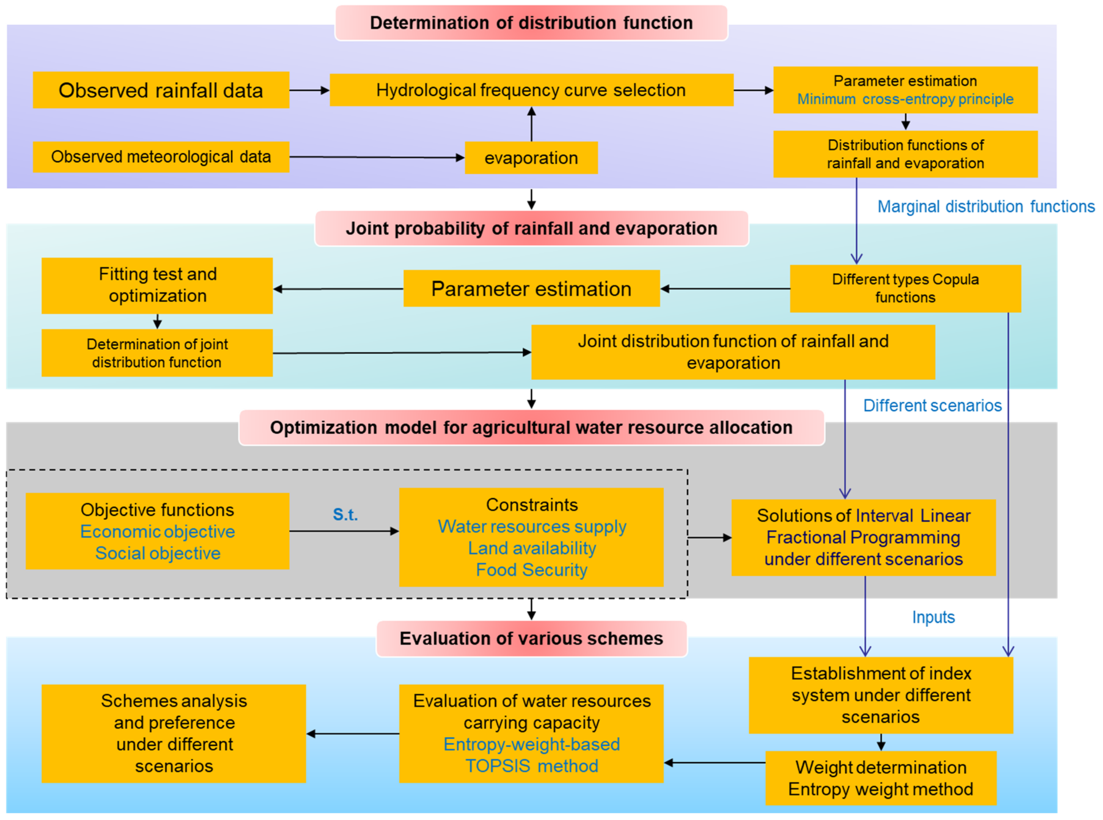
2. Methods
2.1. Minimum Cross-Entropy Principle
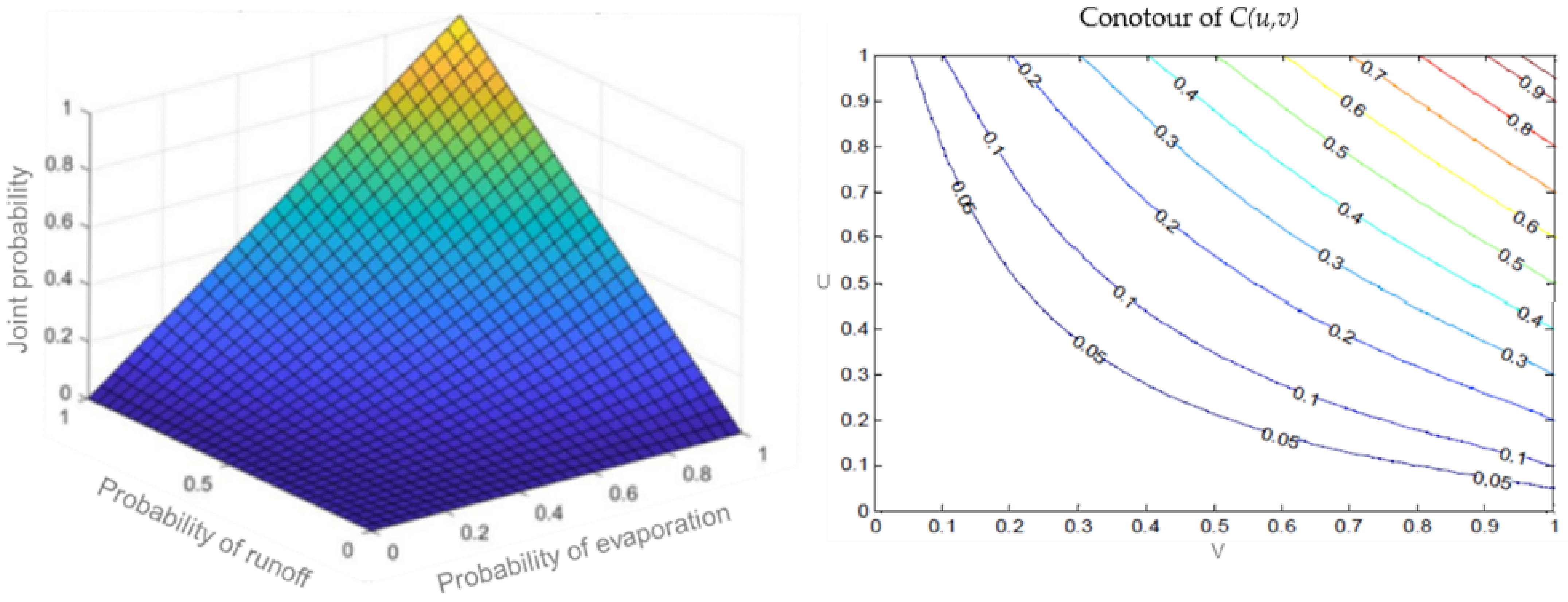
2.2. Copula Function
2.3. Interval Linear Fractional Programming (ILFP)
2.3.1. Interval Parameter Programming (IPP)
2.3.2. Linear Fractional Programming (LFP)
2.3.3. ILFP
2.4. Entropy-Weight-Based TOPSIS Method
3. Application
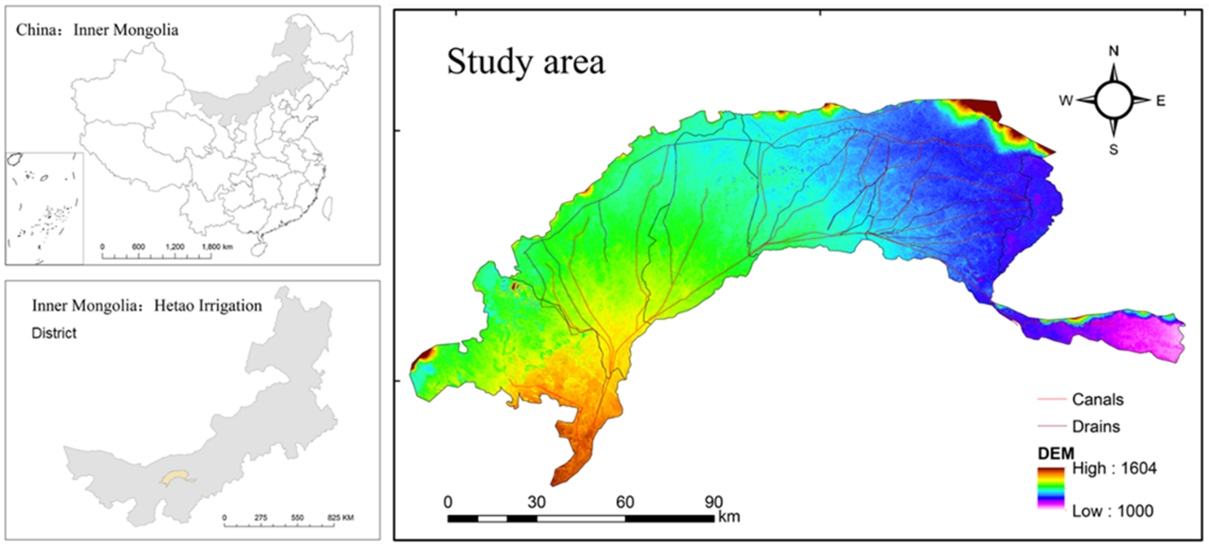
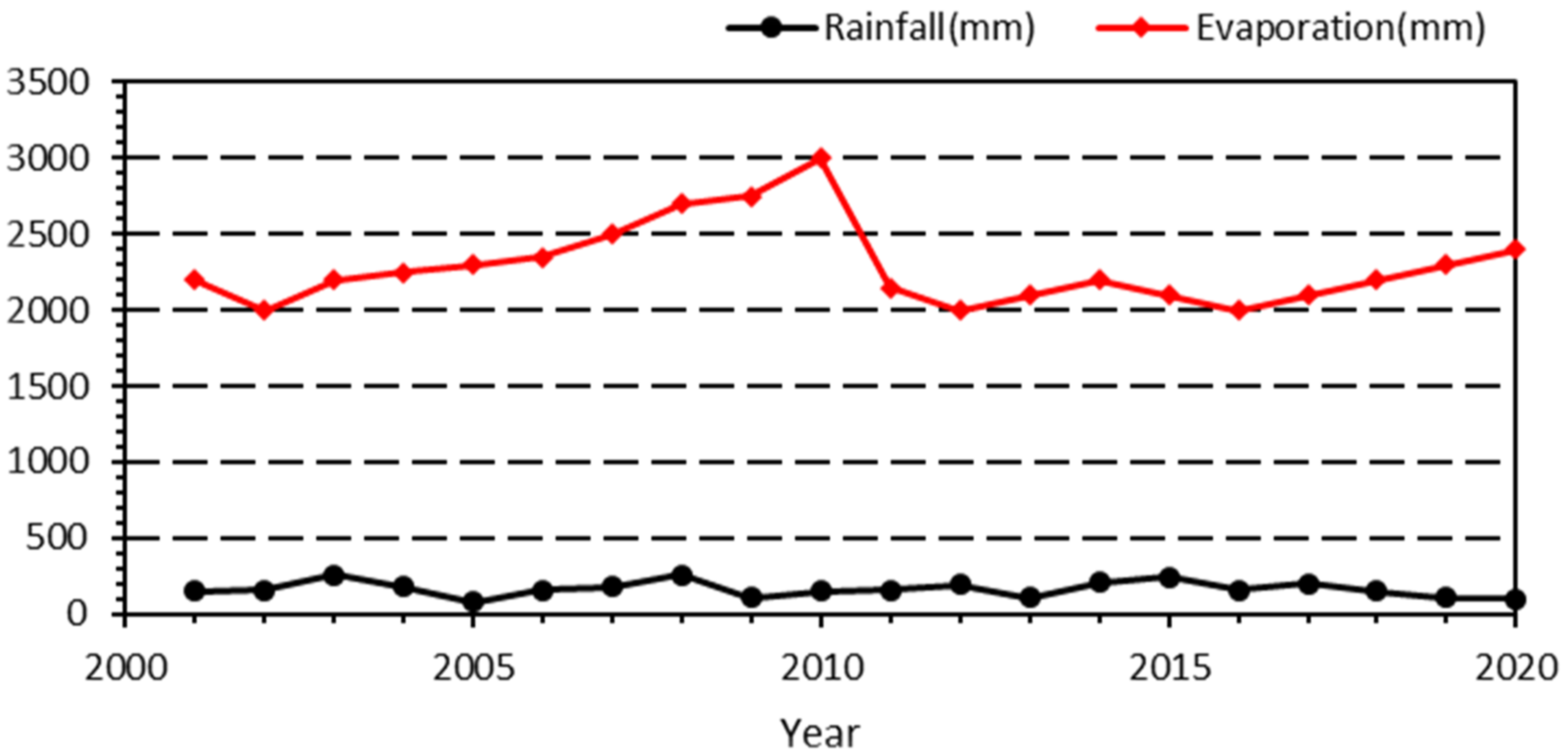
3.1. Study Area and Data Collection
3.2. Parameter Estimation
3.3. Joint Probability of Water Supply and Water Demand
3.4. Agricultural Water Resource Optimal Allocation under Uncertainty
- (1)
- Water availability constraint
- (2)
- Water demand constraint
- (3)
- Land availability constraint
- (4)
- Drip irrigation water quantity constraint
- (5)
- Crop price constraint
- (6)
- Food security constraint
4. Result Analysis and Discussion
4.1. Water Scarcity in the HID
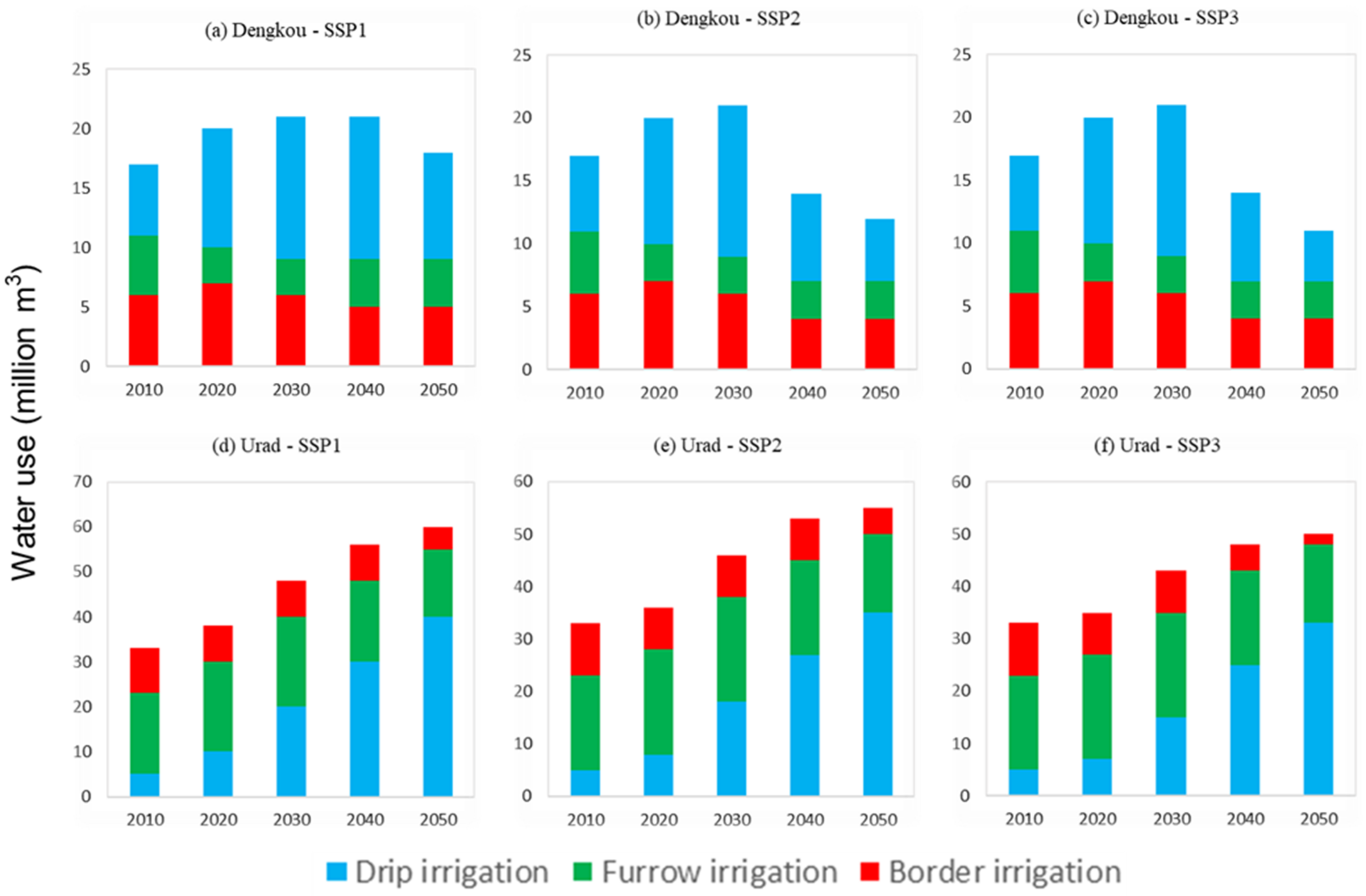
4.2. Regional Water Use in the HID
4.3. Water Availability Changes in the HID
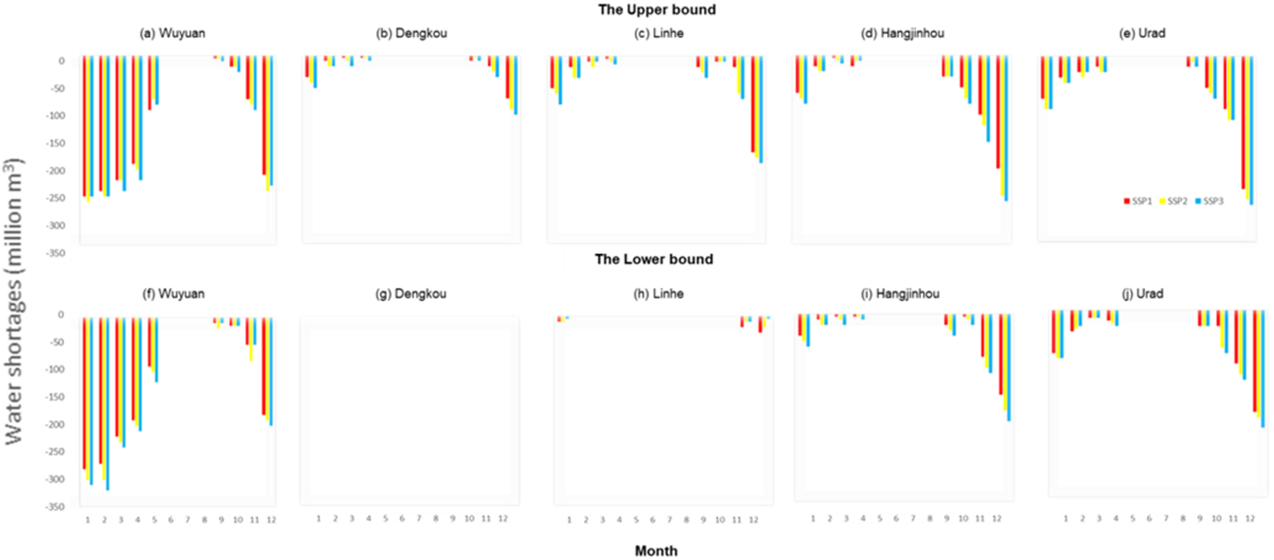
4.4. Water Shortages in the HID
4.5. Evaluation of Water Resources’ Carrying Capacity in the HID
5. Conclusions
Author Contributions
Funding
Conflicts of Interest
Appendix A

| Function Name | C(u,v) | Interpretation |
|---|---|---|
| Clayton copula | and . is the Kendall coefficient of rank correlation, and the same below. | |
| Gumbel copula | and . | |
| Frank copula | and . | |
| t-copula | is the inverse function t distribution function while the degree of freedom is k; ρ is the correlation coefficients between variables. | |
| Gaussian copula | is the inverse function of standard normal distribution function; ρ is the correlation coefficients between variables. |
References
- Li, Y.; Huang, G. An inexact two-stage mixed integer linear programming method for solid waste management in the City of Regina. J. Environ. Manag. 2006, 81, 188–209. [Google Scholar] [CrossRef] [PubMed]
- Huang, G.H.; Chi, G.F.; Li, Y.P. Long-Term Planning of an Integrated Solid Waste Management System under Uncertainty—Ι. Model Development. Environ. Eng. Sci. 2005, 22, 823–834. [Google Scholar] [CrossRef]
- Huang, G.H.; Chi, G.F.; Li, Y.P. Long-Term Planning of an Integrated Solid Waste Management System under Uncertainty—ΙΙ. A North American Case Study. Environ. Eng. Sci. 2005, 22, 835–853. [Google Scholar] [CrossRef]
- Zhang, Y.; Yang, P.; Liu, X.; Adeloye, A.J. Simulation and optimization coupling model for soil salinization and waterlogging control in the Urad irrigation area, North China. J. Hydrol. 2022, 607, 127408. [Google Scholar] [CrossRef]
- Gu, J.J.; Guo, P.; Huang, G.H. Inexact stochastic dynamic programming method and application to water resources management in Shandong China under uncertainty. Stoch. Hydrol. Hydraul. 2013, 27, 1207–1219. [Google Scholar] [CrossRef]
- Gu, J.J.; Guo, P.; Huang, G.H.; Shen, N. Optimization of the industrial structure facing sustainable development in resource-based city subjected to water resources under uncertainty. Stoch. Hydrol. Hydraul. 2013, 27, 659–673. [Google Scholar] [CrossRef]
- Tong, F.; Guo, P. Simulation and optimization for crop water allocation based on crop water production functions and climate factor under uncertainty. Appl. Math. Model. 2013, 37, 7708–7716. [Google Scholar] [CrossRef]
- Li, M.; Guo, P.; Fang, S.Q.; Zhang, L.D. An inexact fuzzy parameter two-stage stochastic programming model for irrigation water allocation under uncertainty. Stoch. Hydrol. Hydraul. 2013, 27, 1441–1452. [Google Scholar] [CrossRef]
- Fang, S.Q.; Guo, P.; Li, M.; Zhang, L. Bi-level Multi-objective Programming Applied to Water Resources Allocation. Math. Prob. Eng. 2013, 2013, 837919. [Google Scholar] [CrossRef] [Green Version]
- Guo, P.; Chen, X.; Tong, L.; Li, J.; Li, M. An optimization model for a crop deficit irrigation system under uncertainty. Eng. Optim. 2012, 46, 1–14. [Google Scholar] [CrossRef]
- Hashimoto, T.; Loucks, D.P.; Stedinger, J.R. Robustness of water resources systems. Water Resour. Res. 1982, 18, 21–26. [Google Scholar] [CrossRef] [Green Version]
- McKinney, D.C.; Loucks, D.P. Network design for predicting groundwater contamination. Water Resour. Res. 1992, 28, 133–147. [Google Scholar] [CrossRef]
- Loucks, D.P. Modeling and managing the interactions between hydrology, ecology and economics. J. Hydrol. 2005, 328, 408–416. [Google Scholar] [CrossRef]
- Revelle, C.S.; Loucks, D.P.; Lynn, W.R. Linear programming applied to water quality management. Water Resour. Res. 1968, 4, 1–9. [Google Scholar] [CrossRef]
- Fedra, K.; Loucks, D.P. Interactive Computer Technology for Planning and Policy Modeling. Water Resour. Res. 1985, 21, 114–122. [Google Scholar] [CrossRef] [Green Version]
- Tan, Q.; Huang, G.H.; Cai, Y.P. Multi-Source Multi-Sector Sustainable Water Supply Under Multiple Uncertainties: An Inexact Fuzzy-Stochastic Quadratic Programming Approach. Water Resour. Manag. 2013, 27, 451–473. [Google Scholar] [CrossRef]
- Tan, Q.; Huang, G.; Cai, Y.; Yang, Z. A non-probabilistic programming approach enabling risk-aversion analysis for supporting sustainable watershed development. J. Clean. Prod. 2016, 112, 4771–4788. [Google Scholar] [CrossRef]
- Tan, Q.; Huang, G.H.; Cai, Y.P. A Fuzzy Evacuation Management Model Oriented Toward the Mitigation of Emissions. J. Environ. Inform. 2015, 25, 117–125. [Google Scholar] [CrossRef] [Green Version]
- Dong, C.; Huang, G.; Tan, Q. A robust optimization modelling approach for managing water and farmland use between anthropogenic modification and ecosystems protection under uncertainties. Ecol. Eng. 2015, 76, 95–109. [Google Scholar] [CrossRef]
- Wang, R.; Li, Y.; Tan, Q. A review of inexact optimization modeling and its application to integrated water resources management. Front. Earth Sci. 2015, 9, 51–64. [Google Scholar] [CrossRef]
- Dong, C.; Huang, G.H.; Tan, Q.; Cai, Y. Coupled planning of water resources and agricultural land-use based on an inexact-stochastic programming model. Front. Ear. Sci. 2014, 8, 70–80. [Google Scholar] [CrossRef]
- Ren, C.; Guo, P.; Li, M.; Li, R. An innovative method for water resources carrying capacity research—Metabolic theory of regional water resources. J. Environ. Manag. 2016, 167, 139–146. [Google Scholar] [CrossRef] [PubMed]
- Ren, C.; Guo, P.; Yang, G.; Li, R.; Liu, L. Spatial and Temporal Analyses of Water Resources Use Efficiency Based on Data Envelope Analysis and Malmquist Index: Case Study in Gansu Province, China. J. Water Resour. Plan. Manag. 2016, 142, 04016066. [Google Scholar] [CrossRef]
- Ren, C.F.; Li, R.H.; Zhang, L.D.; Guo, P. Multi-objective stochastic fractional goal programming model for water resources optimal allocation among industries. J. Water Res. Plan. Manag. 2016, 142, 04016036. [Google Scholar] [CrossRef]
- Ren, C.F.; Guo, P.; Li, M.; Gu, J.J. Optimization of Industrial Structure Considering the Uncertainty of Water Resources. Water Resour. Manag. 2013, 27, 3885–3898. [Google Scholar] [CrossRef]
- Gui, Z.; Zhang, C.; Li, M.; Guo, P. Risk analysis methods of the water resources system under uncertainty. Front. Agric. Sci. Eng. 2015, 2, 205–215. [Google Scholar] [CrossRef]
- Gui, Z.; Li, M.; Guo, P. Simulation-Based Inexact Fuzzy Semi-Infinite Programming Method for Agricultural Cultivated Area Planning in the Shiyang River Basin. J. Irrig. Drain. Eng. 2017, 143, 05016011. [Google Scholar] [CrossRef]
- Guo, P.; Chen, X.; Li, M.; Li, J. Fuzzy chance-constrained linear fractional programming approach for optimal water allocation. Stoch. Hydrol. Hydraul. 2014, 28, 1601–1612. [Google Scholar] [CrossRef]
- Guo, P.; Wang, X.; Zhu, H.; Li, M. Inexact Fuzzy Chance-Constrained Nonlinear Programming Approach for Crop Water Allocation under Precipitation Variation and Sustainable Development. J. Water Resour. Plan. Manag. 2014, 140, 05014003. [Google Scholar] [CrossRef]
- Li, M.; Guo, P.; Liu, X.; Huang, G.; Huo, Z. A decision-support system for cropland irrigation water management and agricultural non-point sources pollution control. Desalination Water Treat. 2014, 52, 5106–5117. [Google Scholar] [CrossRef]
- Zhang, L.D.; Guo, P.; Fang, S.Q.; Li, M. Monthly Optimal Reservoirs Operation for Multi-crop Deficit Irrigation under Fuzzy Stochastic Uncertainties. J. Appl. Math. 2014, 2014, 105391. [Google Scholar]
- Fu, Y.; Li, M.; Guo, P. Optimal Allocation of Water Resources Model for Different Growth Stages of Crops under Uncertainty. J. Irrig. Drain. Eng. 2014, 140, 05014003. [Google Scholar] [CrossRef]
- Zhang, D.; Guo, P. Integrated agriculture water management optimization model for water saving potential analysis. Agric. Water Manag. 2016, 170, 5–19. [Google Scholar] [CrossRef]
- Liu, C.; Rubæk, G.H.; Liu, F.; Andersen, M.N. Effect of partial root zone drying and deficit irrigation on nitrogen and phosphorus uptake in potato. Agric. Water Manag. 2015, 159, 66–76. [Google Scholar] [CrossRef]
- Liu, C.; Liu, F.; Ravnskov, S.; Rubaek, G.H.; Sun, Z.; Andersen, M.N. Impact of Wood Biochar and Its Interactions with Mycorrhizal Fungi, Phosphorus Fertilization and Irrigation Strategies on Potato Growth. J. Agron. Crop Sci. 2016, 203, 131–145. [Google Scholar] [CrossRef]
- Liu, C.; Ravnskov, S.; Liu, F.; Rubæk, G.H.; Andersen, M.N. Arbuscular mycorrhizal fungi alleviate abiotic stresses in potato plants caused by low phosphorus and deficit irrigation/partial root-zone drying. J. Agric. Sci. 2018, 156, 46–58. [Google Scholar] [CrossRef]
- Liu, C.; Liu, F.; Andersen, M.N.; Wang, G.; Wu, K.; Zhao, Q.; Ye, Z. Domestic wastewater infiltration process in desert sandy soil and its irrigation prospect analysis. Ecotoxicol. Environ. Saf. 2020, 208, 111419. [Google Scholar] [CrossRef]
- Huang, W.; Dai, L.M.; Baetz, B.W.; Cao, M.F.; Razavi, S. Interval Binary Programming Model for Noise Control within an Urban Environment. J. Environ. Inform. 2013, 21, 93–101. [Google Scholar] [CrossRef] [Green Version]
- Huang, W.; Walker, W.S.; Kim, Y. Junction potentials in thermolytic reverse electrodialysis. Desalination 2015, 369, 149–155. [Google Scholar] [CrossRef]
- Huang, W.; Baetz, B.W.; Razavi, S. A GIS-Based Integer Programming Approach for the Location of Solid Waste Collection Depots. J. Environ. Inform. 2016, 28, 39–44. [Google Scholar] [CrossRef] [Green Version]
- Huang, W.; Kim, Y. Electrochemical techniques for evaluating short-chain fatty acid utilization by bioanodes. Environ. Sci. Pollut. Res. 2016, 24, 2620–2626. [Google Scholar] [CrossRef] [PubMed]
- Fan, Y.; Huang, W.; Huang, G.; Huang, K.; Zhou, X. A PCM-based stochastic hydrological model for uncertainty quantification in watershed systems. Stoch. Hydrol. Hydraul. 2015, 29, 915–927. [Google Scholar] [CrossRef]
- Fan, Y.R.; Huang, W.; Huang, G.H.; Li, Z.; Li, Y.P.; Wang, X.Q.; Cheng, G.H.; Jin, L. A Stepwise-Cluster Forecasting Approach for Monthly Stream flows Based on Climate Teleconnections. Stoch. Environ. Res. Risk Assess. 2015, 29, 1557–1569. [Google Scholar] [CrossRef]
- Miao, D.Y.; Huang, W.W.; Li, Y.P.; Yang, Z.F. An Inexact Two-Stage Water Quality Management Model for Supporting Sustainable Development in a Rural System. J. Environ. Inform. 2014, 24, 52–64. [Google Scholar]
- Miao, D.Y.; Huang, W.W.; Li, Y.P.; Yang, Z.F. Planning Water Resources Systems under Uncertainty Using An Interval-Fuzzy De Novo Programming Method. J. Environ. Inform. 2014, 24, 11–23. [Google Scholar] [CrossRef] [Green Version]


| Dimension | Index | Unit | Index Attribute | Weights |
|---|---|---|---|---|
| Economic dimension (A) | The benefits of unilateral water (A1) | RMB/m3 | + | 0.1012 |
| Water production efficiency (A2) | kg/ha | + | 0.1058 | |
| Crop output (A3) | RMB | + | 0.1026 | |
| Social dimension (B) | Proportion of green and high-quality agricultural products (B1) | % | + | 0.1324 |
| Land productivity (B2) | kg/ha | + | 0.0988 | |
| Resource consumption per unit of GDP (B3) | kg/RMB | − | 0.1259 | |
| Environmental dimension (C) | Aging rate of engineering facilities (C1) | % | − | 0.0992 |
| Global Warming Potential per output (C2) | kg/CO2e | − | 0.0984 | |
| Agricultural non-point pollution discharge (C3) | kg | − | 0.1357 |
Publisher’s Note: MDPI stays neutral with regard to jurisdictional claims in published maps and institutional affiliations. |
© 2022 by the authors. Licensee MDPI, Basel, Switzerland. This article is an open access article distributed under the terms and conditions of the Creative Commons Attribution (CC BY) license (https://creativecommons.org/licenses/by/4.0/).
Share and Cite
Zhang, Y.; Yang, P. Agricultural Water Optimal Allocation Using Minimum Cross-Entropy and Entropy-Weight-Based TOPSIS Method in Hetao Irrigation District, Northwest China. Agriculture 2022, 12, 853. https://doi.org/10.3390/agriculture12060853
Zhang Y, Yang P. Agricultural Water Optimal Allocation Using Minimum Cross-Entropy and Entropy-Weight-Based TOPSIS Method in Hetao Irrigation District, Northwest China. Agriculture. 2022; 12(6):853. https://doi.org/10.3390/agriculture12060853
Chicago/Turabian StyleZhang, Yunquan, and Peiling Yang. 2022. "Agricultural Water Optimal Allocation Using Minimum Cross-Entropy and Entropy-Weight-Based TOPSIS Method in Hetao Irrigation District, Northwest China" Agriculture 12, no. 6: 853. https://doi.org/10.3390/agriculture12060853