
Simulating the Impacts of Climate Change on Maize Yields Using EPIC: A Case Study in the Eastern Cape Province of South Africa †


Abstract
:1. Introduction
2. Materials and Methods
2.1. Background
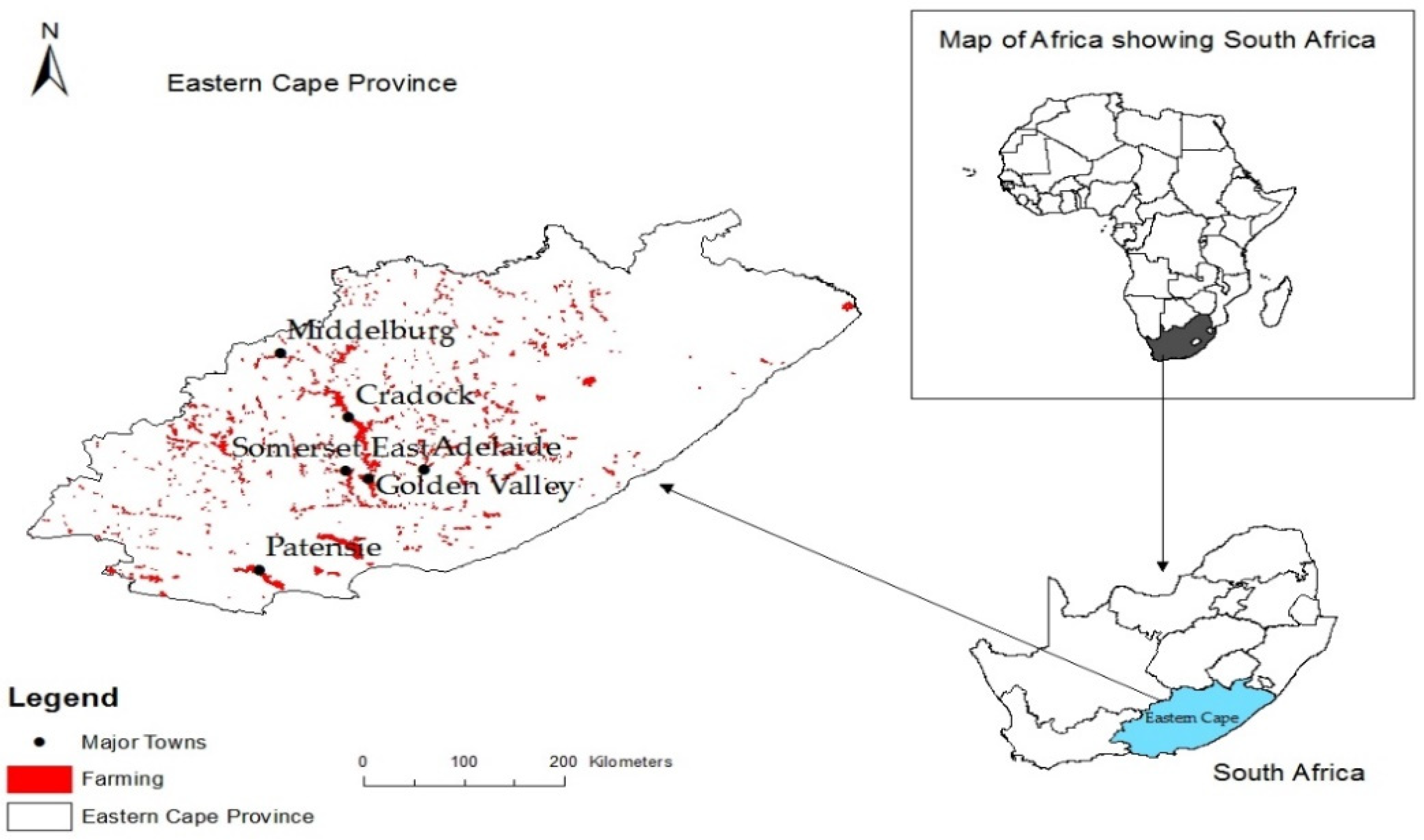
2.2. Study Area
2.3. EPIC Model Description
2.4. Field Work
2.5. Model Inputs
2.6. EPIC Model Set-Up
2.6.1. Framework
2.6.2. Model Calibration
2.6.3. Model Evaluation
2.7. Climate Data
2.8. Data Analysis
3. Results
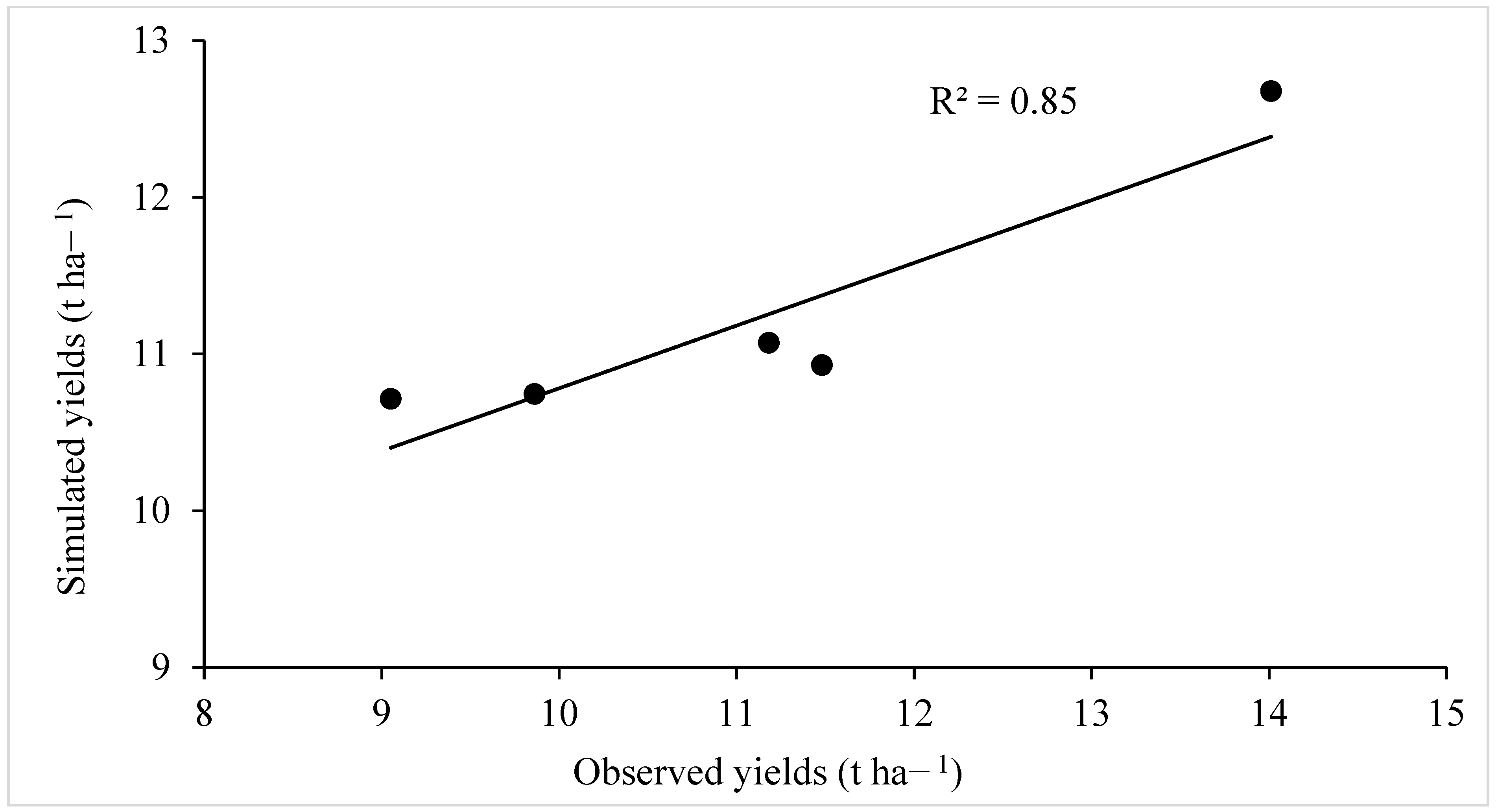
3.1. Model Calibration
3.2. Validation
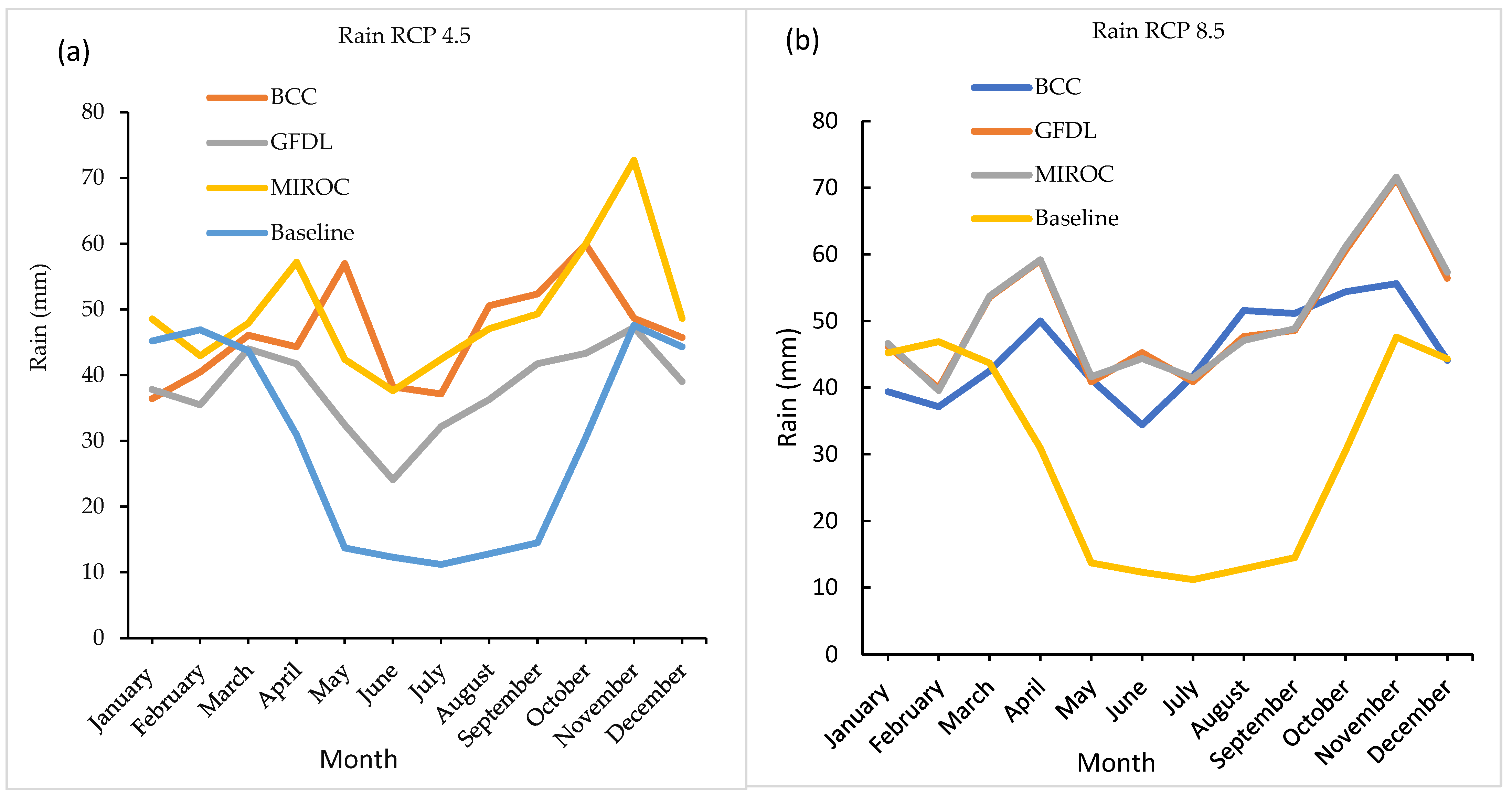
3.3. Climate Data Analysis
3.3.1. Temperature and Rainfall
3.3.2. Yield Simulations
3.3.3. BCC Model
3.3.4. GFDL Model
3.3.5. MIROC Model
4. Discussion
4.1. EPIC Model Calibration and Validation
4.2. Climate Change Impacts on Maize Yield
5. Limitations of the Study
6. Conclusions
Author Contributions
Funding
Institutional Review Board Statement
Informed Consent Statement
Data Availability Statement
Conflicts of Interest
Appendix A

| Soil Parameters | Soil Layer Number | |
|---|---|---|
| 1 | 2 | |
| Bulk density | 1.48 | 1.52 |
| Soil depth | 0.3 | 1.2 |
| Clay | 20.4 | 15.1 |
| Sand | 52.8 | 42.5 |
| Silt | 26.8 | 42.4 |
| pH | 6.5 | 6.5 |
| Soil organic carbon | 0.91 | 0.2 |
| Cation exchange capacity | 14.3 | 13.4 |
| Date 1 | Operation | Type | Amount |
|---|---|---|---|
| 22 October | Planting | Maize | 50,000 plants ha−1 |
| 22 October | Fertilizer application | Superphosphate | 476 kg ha−1 |
| 22 October | Fertilizer application | Ammonium sulfate | 330 kg ha−1 |
| 22 October | Fertilizer application | Calcium sulfate | 120 kg ha−1 |
| 22 October | Irrigation | Furrow | 75 mm |
| 15 November | Fertiliser application | Ammonium sulfate | 300 kg ha−1 |
| 26 November | Irrigation | Furrow | 75 mm |
| 10 December | Fertiliser application | Ammonium sulfate | 300 kg ha−1 |
| 17 December | Irrigation | Furrow | 75 mm |
| 28 December | Irrigation | Furrow | 75 mm |
| 18 January | Irrigation | Furrow | 75 mm |
| 8 February | Irrigation | Furrow | 75 mm |
| 19 February | Irrigation | Furrow | 75 mm |
| 11 March | Irrigation | Furrow | 75 mm |
| 5 June | Harvesting | Manual | 11 tonnes hectare−1 (average) |


References
- Pachauri, R.K.; Allen, M.R.; Barros, V.R.; Broome, J.; Cramer, W.; Christ, R.; Church, J.A.; Clarke, L.; Dahe, Q.; Dasgupta, P.; et al. Climate Change 2014: Synthesis Report. Contribution of Working Groups I, II and III to the Fifth Assessment Report of the Intergovernmental Panel on Climate Change; Pachauri, R.K., Meyer, L.A., Eds.; IPCC: Geneva, Switzerland, 2014. [Google Scholar]
- Long, S.P.; Ainsworth, E.A.; Leakey, A.D.B.; Noösberger, J.; Ort, D.R. Food for Thought: Lower-Than-Expected Crop Yield Stimulation with Rising CO2 Concentrations. Science 2006, 312, 1918–1921. [Google Scholar] [CrossRef] [PubMed]
- Webber, H.; Gaiser, T.; Ewert, F. What role can crop models play in supporting climate change adaptation decisions to enhance food security in Sub-Saharan Africa? Agric. Syst. 2014, 127, 161–177. [Google Scholar] [CrossRef]
- Stuart-Hill, S.; Schulze, R.E.; Colvin, J. Handbook on Adaptive Management Strategies and Options for the Water Sector in S. Afr. under Climate Change; Water Research Commission: Pretoria, South Africa, 2012; ISBN 9781431202706. [Google Scholar]
- Jury, M.R. Climate trends in southern Africa. S. Afr. J. Sci. 2013, 109, 1–11. [Google Scholar] [CrossRef] [Green Version]
- Nhamo, L.; Mabhaudhi, T.; Modi, A. Preparedness or repeated short-term relief aid? Building drought resilience through early warning in southern Africa. Water SA 2019, 45, 75–85. [Google Scholar] [CrossRef] [Green Version]
- Mulungu, K.; Ng’Ombe, J.N. Climate Change Impacts on Sustainable Maize Production in Sub-Saharan Africa: A Review. In Maize-Production and Use; IntechOpen Limited: London, UK, 2020. [Google Scholar] [CrossRef] [Green Version]
- Agbugba, I.K.; Christian, M.; Obi, A. Economic analysis of smallholder maize farmers: Implications for public extension services in Eastern Cape. S. Afr. J. Agric. Ext. 2020, 48, 50–63. [Google Scholar] [CrossRef]
- Chimonyo, V.G.P.; Mutengwa, C.S.; Chiduza, C.; Tandzi, L. Characteristics of maize growing farmers, varietal use and constraints to increase productivity in selected villages in the Eastern Cape province of South Africa. S. Afr. J. Agric. Ext. 2020, 48, 64–82. [Google Scholar] [CrossRef]
- Kogo, B.K.; Kumar, L.; Koech, R.; Langat, P. Modelling Impacts of Climate Change on Maize (Zea mays L.) Growth and Productivity: A Review of Models, Outputs and Limitations. J. Geosci. Environ. Prot. 2019, 7, 76–95. [Google Scholar] [CrossRef] [Green Version]
- Corbeels, M.; Berre, D.; Rusinamhodzi, L.; Lopez-Ridaura, S. Can we use crop modelling for identifying climate change adaptation options? Agric. For. Meteorol. 2018, 256–257, 46–52. [Google Scholar] [CrossRef]
- Jacobson, K. From Betterment to Bt Maize; Swedish University of Agricultural Sciences: Uppsala, Sweden, 2013. [Google Scholar]
- Khapayi, M.; Celliers, P.R. Factors limiting and preventing emerging farmers to progress to commercial agricultural farming in the King William’s Town area of the Eastern Cape Province, South Africa. S. Afr. J. Agric. Ext. (SAJAE) 2016, 44, 25–41. [Google Scholar] [CrossRef] [Green Version]
- Goldblatt, A. Agriculture: Facts and Trends South Africa; World Wide Fund for Nature: Gland, Switzerland, 2011; pp. 2–26. [Google Scholar]
- Uzoma, K.C.; Smith, W.; Grant, B.; Desjardins, R.L.; Gao, X.; Hanis, K.; Tenuta, M.; Goglio, P.; Li, C. Assessing the effects of agricultural management on nitrous oxide emissions using flux measurements and the DNDC model. Agric. Ecosyst. Environ. 2015, 206, 71–83. [Google Scholar] [CrossRef]
- He, W.; Yang, J.Y.; Qian, B.; Drury, C.F.; Hoogenboom, G.; He, P.; Lapen, D.; Zhou, W. Climate change impacts on crop yield, soil water balance and nitrate leaching in the semiarid and humid regions of Canada. PLoS ONE 2018, 13, e0207370. [Google Scholar] [CrossRef] [PubMed]
- Wang, Z.; Qi, Z.; Xue, L.; Bukovsky, M.; Helmers, M.J. Modeling the impacts of climate change on nitrogen losses and crop yield in a subsurface drained field. Clim. Chang. 2015, 129, 323–335. [Google Scholar] [CrossRef] [Green Version]
- Basche, A.; Archontoulis, S.V.; Kaspar, T.C.; Jaynes, D.B.; Parkin, T.B.; Miguez, F.E. Simulating long-term impacts of cover crops and climate change on crop production and environmental outcomes in the Midwestern United States. Agric. Ecosyst. Environ. 2016, 218, 95–106. [Google Scholar] [CrossRef] [Green Version]
- Folberth, C. Modeling Crop Yield and Water Use in the Context of Global Change with a Focus on Maize in Sub-Saharan Africa. Doctoral Thesis, ETH-Zürich, Zürich, Switzerland, 2013. [Google Scholar]
- Warburton, M.; Schulze, R.; Jewitt, G. Hydrological Responses to Combined Land-Use and Climate Change in Three Diverse South African Catchments; IAHS Publication: Wallingford, UK, 2013; Volume 359. [Google Scholar]
- Abraha, M.; Savage, M. Potential impacts of climate change on the grain yield of maize for the midlands of KwaZulu-Natal, South Africa. Agric. Ecosyst. Environ. 2006, 115, 150–160. [Google Scholar] [CrossRef]
- Navarro-Racines, C.E.; Tarapues, J.; Thornton, P.; Jarvis, A.; Ramirez-Villegas, J. High-resolution and bias-corrected CMIP5 projections for climate change impact assessments. Sci. Data 2020, 7, 1–14. [Google Scholar] [CrossRef] [PubMed] [Green Version]
- Tang, J.; Niu, X.; Wang, S.; Gao, H.; Wang, X.; Wu, J. Statistical downscaling and dynamical downscaling of regional climate in China: Present climate evaluations and future climate projections. J. Geophys. Res. Atmos. 2016, 121, 2110–2129. [Google Scholar] [CrossRef] [Green Version]
- Kaini, S.; Nepal, S.; Pradhananga, S.; Gardner, T.; Sharma, A.K. Representative general circulation models selection and downscaling of climate data for the transboundary Koshi river basin in China and Nepal. Int. J. Clim. 2020, 40, 4131–4149. [Google Scholar] [CrossRef] [Green Version]
- Ziervogel, G.; Shale, M.; DU, M. Climate change adaptation in a developing country context: The case of urban water supply in Cape Town. Clim. Dev. 2010, 2, 94–110. [Google Scholar] [CrossRef]
- Tisseuil, C.; Vrac, M.; Lek, S.; Wade, A. Statistical downscaling of river flows. J. Hydrol. 2010, 385, 279–291. [Google Scholar] [CrossRef]
- Tadross, M.; Jack, C.; Hewitson, B. On RCM-based projections of change in southern African summer climate. Geophys. Res. Lett. 2005, 32. [Google Scholar] [CrossRef]
- Oosthuizen, H.; Schulze, R.; Crespo, O.; Louw, D.; Tadross, M.; Waagsaether, K.; Arowolo, S. Modelling Impacts of Climate Change on Selected South African Crop Farming Sysytems; Water Research Commission: Gezina, South Africa, 2016. [Google Scholar]
- Siabi, E.K.; Kabobah, A.T.; Akpoti, K.; Anornu, G.K.; Amo-Boateng, M.; Nyantakyi, E.K. Statistical downscaling of global circulation models to assess future climate changes in the Black Volta basin of Ghana. Environ. Chall. 2021, 5, 100299. [Google Scholar] [CrossRef]
- Johnson, K.A.; Smithers, J.C.; E Schulze, R. A review of methods to account for impacts of non-stationary climate data on extreme rainfalls for design rainfall estimation in South Africa. J. S. Afr. Inst. Civ. Eng. 2021, 63, 55–61. [Google Scholar] [CrossRef]
- Ziervogel, G.; New, M.; van Garderen, E.A.; Midgley, G.; Taylor, A.; Hamann, R.; Stuart-Hill, S.; Myers, J.; Warburton, M. Climate change impacts and adaptation in South Africa. WIREs Clim. Chang. 2014, 5, 605–620. [Google Scholar] [CrossRef]
- Choruma, D.J.; Balkovic, J.; Odume, O.N. Calibration and Validation of the EPIC Model for Maize Production in the Eastern Cape, South Africa. Agronomy 2019, 9, 494. [Google Scholar] [CrossRef] [Green Version]
- USDA-Natural Resources Conservation Service. Soil Survey Staff Keys to Soil Taxonomy, 12th ed.; USDA-Natural Resources Conservation Service: Washington, DC, USA, 2014. [Google Scholar]
- Mahlalela, P.T.; Blamey, R.C.; Hart, N.; Reason, C.J.C. Drought in the Eastern Cape region of South Africa and trends in rainfall characteristics. Clim. Dyn. 2020, 55, 2743–2759. [Google Scholar] [CrossRef]
- Department of Environmental Affairs Long-Term Adaptation Scenarios Flagship Research Programme (LTAS) for South Africa. Climate Change Implications for the Water Sector in South Africa; SANBI: Pretoria, South Africa, 2013; Volume 1.
- Williams, J.R.; Gerik, T.; Dagitz, S.; Magre, M.; Meinardus, A.; Steglich, E.; Taylor, R. Environmental Policy Integrated Climate Model-Users Manual Version 0810; Blackland Research and Extension Centre: Temple, TX, USA, 2015. [Google Scholar]
- Xiong, W.; Skalský, R.; Porter, C.H.; Balkovič, J.; Jones, J.W.; Yang, D. Calibration-induced uncertainty of the EPIC model to estimate climate change impact on global maize yield. J. Adv. Model. Earth Syst. 2016, 8, 1358–1375. [Google Scholar] [CrossRef] [Green Version]
- Rinaldi, M.; De Luca, D. Application of EPIC model to assess climate change impact on sorghum in southern Italy. Ital. J. Agron. 2012, 7, 12. [Google Scholar] [CrossRef] [Green Version]
- Balkovic, J.; van der Velde, M.; Schmid, E.; Skalský, R.; Khabarov, N.; Obersteiner, M.; Stürmer, B.; Xiong, W. Pan-European crop modelling with EPIC: Implementation, up-scaling and regional crop yield validation. Agric. Syst. 2013, 120, 61–75. [Google Scholar] [CrossRef]
- Clewer, A.G.; Scarisbrick, D.H. Practical Statistics and Experimental Design for Plant and Crop Science; Wiley: Hoboken, NJ, USA, 2001; ISBN 9780471899082. [Google Scholar]
- Ruane, A.C.; Goldberg, R.; Chryssanthacopoulos, J. Climate forcing datasets for agricultural modeling: Merged products for gap-filling and historical climate series estimation. Agric. For. Meteorol. 2015, 200, 233–248. [Google Scholar] [CrossRef] [Green Version]
- FAO; IIASA; ISRIC; ISS-CAS; JRC. Harmonized World Soil Database; Version 1.1; FAO: Rome, Italy; Laxenburg, Austria, 2009. [Google Scholar]
- Balkovič, J.; van der Velde, M.; Skalský, R.; Xiong, W.; Folberth, C.; Khabarov, N.; Smirnov, A.; Mueller, N.D.; Obersteiner, M. Global wheat production potentials and management flexibility under the representative concentration pathways. Glob. Planet. Chang. 2014, 122, 107–121. [Google Scholar] [CrossRef] [Green Version]
- Schulze, R.; Maharaj, M. A-Pan Equivalent Reference Potential Evaporation; Schulze, R.E., Ed.; University of KwaZulu-Natal: Durban, South Africa, 2007. [Google Scholar]
- Bao, Y.; Hoogenboom, G.; McClendon, R.; Vellidis, G. A comparison of the performance of the CSM-CERES-Maize and EPIC models using maize variety trial data. Agric. Syst. 2017, 150, 109–119. [Google Scholar] [CrossRef] [Green Version]
- Moriasi, D.N.; Arnold, J.G.; van Liew, M.W.; Bingner, R.L.; Harmel, R.D.; Veith, T.L. Model Evaluation Guidelines for Systematic Quantification of Accuracy in Watershed Simulations. Trans. ASABE 2007, 50, 885–900. [Google Scholar] [CrossRef]
- Gupta, H.V.; Sorooshian, S.; Yapo, P.O. Status of Automatic Calibration for Hydrologic Models: Comparison with Multilevel Expert Calibration. J. Hydrol. Eng. 1999, 4, 135–143. [Google Scholar] [CrossRef]
- Wang, X.; Williams, J.R.; Gassman, P.W.; Baffaut, C.; Izaurralde, R.; Jeong, J.; Kiniry, J.R. EPIC and APEX: Model Use, Calibration, and Validation. Trans. ASABE 2012, 55, 1447–1462. [Google Scholar] [CrossRef]
- Taylor, K.E.; Stouffer, R.J.; Meehl, G.A. An Overview of CMIP5 and the Experiment Design. Bull. Am. Meteorol. Soc. 2012, 93, 485–498. [Google Scholar] [CrossRef] [Green Version]
- Mackellar, N.; New, M.; Jack, C. Observed and modelled trends in rainfall and temperature for South Africa: 1960–2010. S. Afr. J. Sci. 2014, 110, 1–13. [Google Scholar] [CrossRef] [Green Version]
- Lekalakala, G. Options for Managing Climate Risk and Climate Change Adaptation in Smallholder Farming Systems of the Limpopo Province, South Africa. Ph.D. Thesis, Georg-August-University Göttingen, Göttingen, Germany, 2017. [Google Scholar]
- Wise, M.; Calvin, K.; Thomson, A.; Clarke, L.; Bond-Lamberty, B.; Sands, R.; Smith, S.J.; Janetos, A.; Edmonds, J. Implications of Limiting CO2 Concentrations for Land Use and Energy. Science 2009, 324, 1183–1186. [Google Scholar] [CrossRef]
- Smith, S.J.; Wigley, T. Multi-Gas Forcing Stabilization with Minicam. Energy J. 2006, 27, 373–391. [Google Scholar] [CrossRef]
- Riahi, K.; Rao, S.; Krey, V.; Cho, C.; Chirkov, V.; Fischer, G.; Kindermann, G.E.; Nakicenovic, N.; Rafaj, P. RCP 8.5—A scenario of comparatively high greenhouse gas emissions. Clim. Chang. 2011, 109, 33–57. [Google Scholar] [CrossRef] [Green Version]
- Niu, X.; Easterling, W.; Hays, C.J.; Jacobs, A.; Mearns, L. Reliability and input-data induced uncertainty of the EPIC model to estimate climate change impact on sorghum yields in the U.S. Great Plains. Agric. Ecosyst. Environ. 2009, 129, 268–276. [Google Scholar] [CrossRef]
- Xiong, W.; Balkovič, J.; van der Velde, M.; Zhang, X.; Izaurralde, R.; Skalský, R.; Lin, E.; Mueller, N.; Obersteiner, M. A calibration procedure to improve global rice yield simulations with EPIC. Ecol. Model. 2014, 273, 128–139. [Google Scholar] [CrossRef]
- Angulo, C.; Rötter, R.; Lock, R.; Enders, A.; Fronzek, S.; Ewert, F. Implication of crop model calibration strategies for assessing regional impacts of climate change in Europe. Agric. For. Meteorol. 2013, 170, 32–46. [Google Scholar] [CrossRef]
- Williams, J.R.; Jones, C.A.; Kiniry, J.R.; Spanel, D.A. The EPIC Crop Growth Model. Trans. ASAE 1989, 32, 0497–0511. [Google Scholar] [CrossRef]
- du Plessis, J. Maize Production; Department of Agriculture: Pretoria, South Africa, 2003.
- Folberth, C.; Yang, H.; Gaiser, T.; Abbaspour, K.C.; Schulin, R. Modeling maize yield responses to improvement in nutrient, water and cultivar inputs in sub-Saharan Africa. Agric. Syst. 2013, 119, 22–34. [Google Scholar] [CrossRef]
- Kiniry, J.R.; Williams, J.R.; Vanderlip, R.L.; Atwood, J.D.; Reicosky, D.C.; Mulliken, J.; Cox, W.J.; Mascagni, H.J.; Hollinger, S.E.; Wiebold, W.J. Evaluation of Two Maize Models for Nine U.S. Locations. Agron. J. 1997, 89, 421–426. [Google Scholar] [CrossRef]
- Wang, X.C.; Li, J.; Tahir, M.N.; De Hao, M. Validation of the EPIC model using a long-term experimental data on the semi-arid Loess Plateau of China. Math. Comput. Model. 2011, 54, 976–986. [Google Scholar] [CrossRef]
- Wang, X.; He, X.; Williams, J.R.; Izaurralde, R.; Atwood, J.D. Sensitivity an Uncertainity Analysis of Crop Yields and Soil Organic Carbon Simulated with EPIC. Trans. ASAE 2005, 48, 1041–1054. [Google Scholar] [CrossRef]
- Martin, S.M.; Nearing, M.A.; Bruce, R.R. An Evaluation of the EPIC Model for Soybeans Grown in Southern Piedmont Soils. Trans. ASAE 1993, 36, 1327–1331. [Google Scholar] [CrossRef]
- Warner, G.; Stake, J.; Guillard, K. Evaluation of EPIC for a Shallow New England Soil: I. Maize Yield and Nitrogen Uptake. Trans. ASABE 1997, 40, 575–583. [Google Scholar] [CrossRef]
- Kiniry, J.R.; Williams, J.R.; Major, D.J.; Izaurralde, R.C.; Gassman, P.W.; Morrison, M.; Bergentine, R.; Zentner, R.P. EPIC model parameters for cereal, oilseed, and forage crops in the northern Great Plains region. Can. J. Plant Sci. 1995, 75, 679–688. [Google Scholar] [CrossRef]
- Ko, J.; Piccinni, G.; Steglich, E. Using EPIC model to manage irrigated cotton and maize. Agric. Water Manag. 2009, 96, 1323–1331. [Google Scholar] [CrossRef]
- Craufurd, P.Q.; Wheeler, T.R. Climate change and the flowering time of annual crops. J. Exp. Bot. 2009, 60, 2529–2539. [Google Scholar] [CrossRef] [PubMed] [Green Version]
- Dominguez-Faus, R.; Folberth, C.; Liu, J.; Jaffe, A.M.; Alvarez, P.J.J. Climate Change Would Increase the Water Intensity of Irrigated Corn Ethanol. Environ. Sci. Technol. 2013, 47, 6030–6037. [Google Scholar] [CrossRef] [PubMed]
- Sacks, W.J.; Deryng, D.; Foley, J.A.; Ramankutty, N. Crop planting dates: An analysis of global patterns. Glob. Ecol. Biogeogr. 2010, 19, 607–620. [Google Scholar] [CrossRef]
- Matarira, C.H.; Makadho, J.M.; Mwamuka, F.C. Climate Change Impacts on Maize Production and Adaptive Measures for the Agricultural Sector. In Interim Report on Climate Change Country Studies; Ramos-Mane, C., Benioff, R., Eds.; US Country Studies Program: Washington, DC, USA, 1995. [Google Scholar]
- Walker, N.; Schulze, R. An assessment of sustainable maize production under different management and climate scenarios for smallholder agro-ecosystems in KwaZulu-Natal, South Africa. Phys. Chem. Earth Parts A/B/C 2006, 31, 995–1002. [Google Scholar] [CrossRef]
- Araya, A.; Kisekka, I.; Lin, X.; Prasad, P.V.; Gowda, P.; Rice, C.; Andales, A. Evaluating the impact of future climate change on irrigated maize production in Kansas. Clim. Risk Manag. 2017, 17, 139–154. [Google Scholar] [CrossRef]
- Bassu, S.; Brisson, N.; Durand, J.-L.; Boote, K.; Lizaso, J.; Jones, J.W.; Rosenzweig, C.; Ruane, A.C.; Adam, M.; Baron, C.; et al. How do various maize crop models vary in their responses to climate change factors? Glob. Chang. Biol. 2014, 20, 2301–2320. [Google Scholar] [CrossRef]
- Islam, A.; Ahuja, L.R.; Garcia, L.A.; Ma, L.; Saseendran, A.S.; Trout, T. Modeling the impacts of climate change on irrigated corn production in the Central Great Plains. Agric. Water Manag. 2012, 110, 94–108. [Google Scholar] [CrossRef]
- Olesen, J.E.; Bindi, M. Consequences of climate change for European agricultural productivity, land use and policy. Eur. J. Agron. 2002, 16, 239–262. [Google Scholar] [CrossRef]
- Yin, G.; Gu, J.; Zhang, F.; Hao, L.; Cong, P.; Liu, Z. Maize Yield Response to Water Supply and Fertilizer Input in a Semi-Arid Environment of Northeast China. PLoS ONE 2014, 9, e86099. [Google Scholar] [CrossRef] [Green Version]
- Durodola, O.S.; Mourad, K.A. Modelling Maize Yield and Water Requirements under Different Climate Change Scenarios. Climate 2020, 8, 127. [Google Scholar] [CrossRef]
- Chisanga, C.B.; Phiri, E.; Chinene, V.R.N.; Chabala, L.M. Projecting maize yield under local-scale climate change scenarios using crop models: Sensitivity to sowing dates, cultivar, and nitrogen fertilizer rates. Food Energy Secur. 2020, 9. [Google Scholar] [CrossRef]
- Mapfumo, P.; Chagwiza, C.; Antwi, M. Impact of Rainfall Variability on Maize Yield in the KwaZulu-Natal, North-West and Free State Provinces of South Africa (1987–2017). J. Agribus. Rural. Dev. 2020, 58, 359–367. [Google Scholar] [CrossRef]
- Mnkeni, P.; Chiduza, C.; Modi, A.T.; Stevens, J.B. Best Management Practices for Smallholder Farming on Two Irrigation Schemes in the Eastern Cape and Kwazulu-Natal Through Participatory Adaptive Research; Water Research Commission: Pretoria, South Africa, 2010. [Google Scholar]
- Jury, M.R. Climate trends across South Africa since 1980. Water SA 2018, 44, 297–307. [Google Scholar] [CrossRef] [Green Version]
- Davis-Reddy, C.L.; Vincent, K. Climate Change Handbook for Southern Africa Climate, 2nd ed.; CSIR: Pretoria, South Africa, 2017; ISBN 9780620765220. [Google Scholar]
- Wang, J.; Wang, E.L.; Yang, X.G.; Zhang, F.S.; Yin, H. Increased yield potential of wheat-maize cropping system in the North China Plain by climate change adaptation. Clim. Chang. 2012, 113, 825–840. [Google Scholar] [CrossRef]
- Yang, Y.; Liu, D.L.; Anwar, M.R.; Zuo, H.; Yang, Y. Impact of future climate change on wheat production in relation to plant-available water capacity in a semiaridenvironment. Arch. Meteorol. Geophys. Bioclimatol. Ser. B 2013, 115, 391–410. [Google Scholar] [CrossRef]
- Müller, C.; Waha, K.; Bondeau, A.; Heinke, J. Hotspots of climate change impacts in sub-Saharan Africa and implications for adaptation and development. Glob. Chang. Biol. 2014, 20, 2505–2517. [Google Scholar] [CrossRef]
- Dale, A.L.; Fant, C.W.; Strzepek, K.; Lickley, M.J.; Solomon, S. Climate model uncertainty in impact assessments for agriculture: A multi-ensemble case study on maize in sub-Saharan Africa. Earth’s Futur. 2017, 5, 337–353. [Google Scholar] [CrossRef]
- Asseng, S.; Ewert, F.; Rosenzweig, C.; Jones, J.W.; Hatfield, J.L.; Ruane, A.C.; Boote, K.; Thorburn, P.J.; Rötter, R.; Cammarano, D.; et al. Uncertainty in simulating wheat yields under climate change. Nat. Clim. Chang. 2013, 3, 827–832. [Google Scholar] [CrossRef] [Green Version]
- Klein, T.; Holzkämper, A.; Calanca, P.; Seppelt, R.; Fuhrer, J. Adapting agricultural land management to climate change: A regional multi-objective optimization approach. Landsc. Ecol. 2013, 28, 2029–2047. [Google Scholar] [CrossRef] [Green Version]
- Ceglar, A.; Črepinšek, Z.; Kajfež-Bogataj, L.; Pogačar, T. The simulation of phenological development in dynamic crop model: The Bayesian comparison of different methods. Agric. For. Meteorol. 2011, 151, 101–115. [Google Scholar] [CrossRef]
- van der Linden, P.; Mitchell, J. Ensembles: Climate Change and Its Impact: Summary of Research and the Results from the ENSEMBLES Project. Met Off. Hadley Cent. Exeter 2009. [Google Scholar] [CrossRef]
- Parry, M.L.; Rosenzweig, C.; Iglesias, A.; Livermore, M.; Fischer, G. Effects of climate change on global food production under SRES emissions and socio-economic scenarios. Glob. Environ. Chang. 2004, 14, 53–67. [Google Scholar] [CrossRef]
- Swann, A.L.S.; Hoffman, F.M.; Koven, C.D.; Randerson, J.T. Plant responses to increasing CO2 reduce estimates of climate impacts on drought severity. Proc. Natl. Acad. Sci. USA 2016, 113, 10019–10024. [Google Scholar] [CrossRef] [Green Version]
- Mengis, N.; Keller, D.P.; Eby, M.; Oschlies, A. Uncertainty in the response of transpiration to CO2 and implications for climate change. Environ. Res. Lett. 2015, 10, 094001. [Google Scholar] [CrossRef]
- Biernath, C.; Gayler, S.; Bittner, S.; Klein, C.; Högy, P.; Fangmeier, A.; Priesack, E. Evaluating the ability of four crop models to predict different environmental impacts on spring wheat grown in open-top chambers. Eur. J. Agron. 2011, 35, 71–82. [Google Scholar] [CrossRef] [Green Version]


| Driving Regional General Circulation Model | Source | Abbreviation of the Model Used in this Study |
|---|---|---|
| BCC-CSM1.1 | Beijing Climate Centre, China Meteorological Administration, China | BCC |
| GFDL-ESM2M | Geophysical Fluid Dynamic Laboratory, USA | GFDL |
| MIROC-ESM | Atmosphere and Ocean Research Institute (University of Tokyo), National Institute for Environmental Studies and Japan Agency for Marine-Earth Science and Technology | MIROC |
| Observed Mean (t ha−1) | Simulated Mean (t ha−1) | NSE | RMSE (t ha−1) | PBIAS % | |
|---|---|---|---|---|---|
| Calibration | 11.26 | 11.23 | 0.53 | 1.17 | 0.31 |
| Validation | 11.12 | 11.23 | 0.61 | 1.018 | −0.2 |
| Yield (t ha−1) | Irrigation Water Used (mm) | WUE (kg ha−1 mm−1) | N Leaching (kg N ha−1) | Seasonal Et (mm) | |
|---|---|---|---|---|---|
| Scenario | |||||
| Baseline | 12.24 A ± 0.58 | 562.89 A ± 82.53 | 24.13 A ± 1.33 | 19.91 B ± 24.17 | 907.78 C ± 46.79 |
| RCP 4.5 | 11.51 B ± 1.10 | 541.09 A ± 74.29 | 23.46 A ± 1.96 | 36.79 B ± 34.09 | 943.10 A ± 39.08 |
| RCP 8.5 | 10.20 C ± 0.81 | 460.81 B ± 61.86 | 22.40 B ± 1.19 | 66.13 A ± 53.58 | 918.84 B ± 40.94 |
| General Circulation Model | |||||
| BCC-ESM | 10.89 A ± 1.17 | 509.23 A ± 66.43 | 23.24 A ± 2.34 | 49.22 A ± 41.35 | 922.45 A ± 32.91 |
| GFDL | 11.05 A ± 1.32 | 510.82 A ± 92.8 | 22.95 B ± 1.33 | 47.34 A ± 52.37 | 933.88 A ± 45.78 |
| MIROC | 10.62 A ± 0.95 | 481.52 A ± 73.55 | 22.58 BC ± 1.09 | 56.49 A ± 48.18 | 936.34 A ± 44.62 |
| Period | |||||
| 2040–2069 | 11.31 * ± 0.73 | 525.26 *±6 8.77 | 23.37 * ± 0.76 | 39.35 * ± 34.14 | 938.76 * ± 36.59 |
| 2070–2099 | 10.39 * ± 1.33 | 475.82 * ± 81.78 | 22.48 * ± 1.33 | 62.78 * ± 55.77 | 922.62 * ± 45.13 |
| Scenario and Period | Yield | Seasonal Irrigation | Water Use Efficiency | N Leaching |
|---|---|---|---|---|
| BCC | ||||
| RCP 4.5 2040–2069 | −8.2 | −5.4 | −4.3 | −26.4 |
| RCP 4.5 2070–2099 | −7.4 | −5.9 | −5.1 | 108.8 |
| RCP 8.5 2040–2069 | −10.7 | −5.9 | −7.0 | 148.4 |
| RCP 8.5 2070–2099 | −15.6 | −8.0 | −14.1 | 215.5 |
| GFDL | ||||
| RCP 4.5 2040–2069 | 0.0 | −1.9 | 0 | 17.4 |
| RCP 4.5 2070–2099 | −2.5 | 0.3 | −2.8 | 39.4 |
| RCP 8.5 2040–2069 | −14.8 | −13.6 | −13.4 | 207.5 |
| RCP 8.5 2070–2099 | −20.8 | −13.6 | −21.7 | 375.4 |
| MIROC | ||||
| RCP 4.5 2040–2069 | −8.2 | −13.2 | −6.6 | 113.5 |
| RCP 4.5 2070–2099 | −13.1 | −8.7 | −12.1 | 178.8 |
| RCP 8.5 2040–2069 | −10.7 | −12.9 | −9.6 | 153.2 |
| RCP 8.5 2070–2099 | −23.8 | −13.6 | −22.7 | 373.8 |
Publisher’s Note: MDPI stays neutral with regard to jurisdictional claims in published maps and institutional affiliations. |
© 2022 by the authors. Licensee MDPI, Basel, Switzerland. This article is an open access article distributed under the terms and conditions of the Creative Commons Attribution (CC BY) license (https://creativecommons.org/licenses/by/4.0/).
Share and Cite
Choruma, D.J.; Akamagwuna, F.C.; Odume, N.O. Simulating the Impacts of Climate Change on Maize Yields Using EPIC: A Case Study in the Eastern Cape Province of South Africa. Agriculture 2022, 12, 794. https://doi.org/10.3390/agriculture12060794
Choruma DJ, Akamagwuna FC, Odume NO. Simulating the Impacts of Climate Change on Maize Yields Using EPIC: A Case Study in the Eastern Cape Province of South Africa. Agriculture. 2022; 12(6):794. https://doi.org/10.3390/agriculture12060794
Chicago/Turabian StyleChoruma, Dennis Junior, Frank Chukwuzuoke Akamagwuna, and Nelson Oghenekaro Odume. 2022. "Simulating the Impacts of Climate Change on Maize Yields Using EPIC: A Case Study in the Eastern Cape Province of South Africa" Agriculture 12, no. 6: 794. https://doi.org/10.3390/agriculture12060794