
Research on the Time-Dependent Split Delivery Green Vehicle Routing Problem for Fresh Agricultural Products with Multiple Time Windows


Abstract
:1. Introduction
- (1)
- Split delivery vehicle routing problem with multiple time windows
- (2)
- The Distribution of Fresh Agricultural Products
- (3)
- Time-Dependent Vehicle Routing Problem
- The SDVRPTW model has been applied rarely in the research of fresh agricultural product distribution. The basic SDVRPTW model normally takes into account load constraints, split delivery and the precondition that the consumer has just one time window. In order to make the model better simulate the actual conditions of fresh agricultural product distribution, this study will consider and evaluate a time-varying road network, carbon emissions and customer satisfaction on the basis of SDVRPTW to develop the TDSDGVRPMTW model.
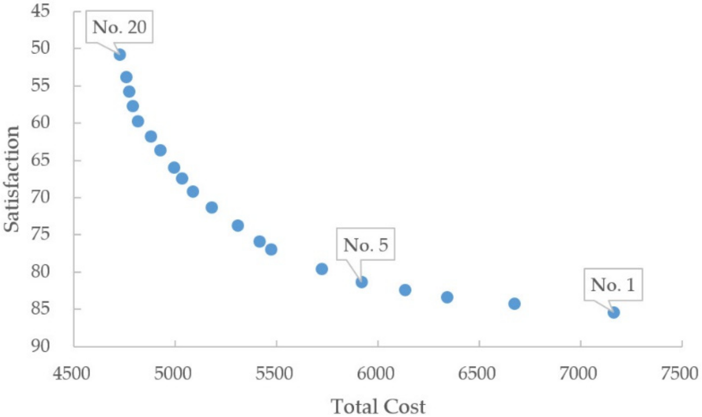
- While multi-objective optimization problems are frequently aimed at obtaining a Pareto-optimal front, decision-makers expect a complete and feasible solution. Furthermore, the TOPSIS method is employed to select the solution that satisfies the requirements from the Pareto-optimal front.
- It is verified by a real-world case that as a delivery strategy, the TDSDGVRPMTW model proposed in this paper not only can effectively reduce the total cost of fresh agricultural products distribution, but also improve customer satisfaction.
- The customer’s demand for fresh agricultural products is split and distributed according to the temperature required for distribution, and each customer has multiple time windows for receiving services.
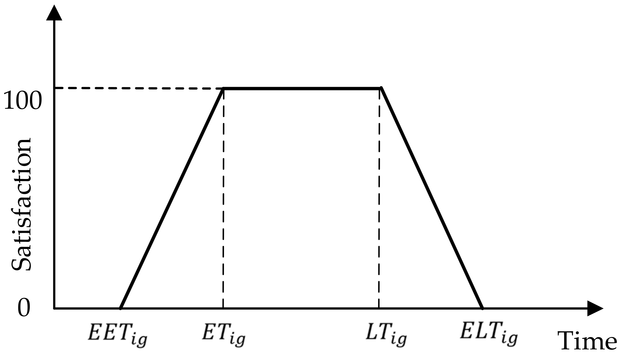
- For each service, every customer will complete a satisfaction rating, the value of satisfaction evaluation depends on the deviation degree between the remaining time when the vehicle leaves the customer and the time window.
- Only one type of produce can be delivered by a single vehicle. A vehicle can only serve a customer once.
- The day is divided into several time periods, and vehicles travel at various speeds at different periods.
2. Materials and Methods
2.1. TDSDGVRPMTW Model
- The travel cost
- The fixed cost
- The service cost
- The refrigeration cost
- The carbon cost
2.2. Customer Satisfaction Measurement Method
2.3. Time-Dependent Vehicle Speed Calculation Method
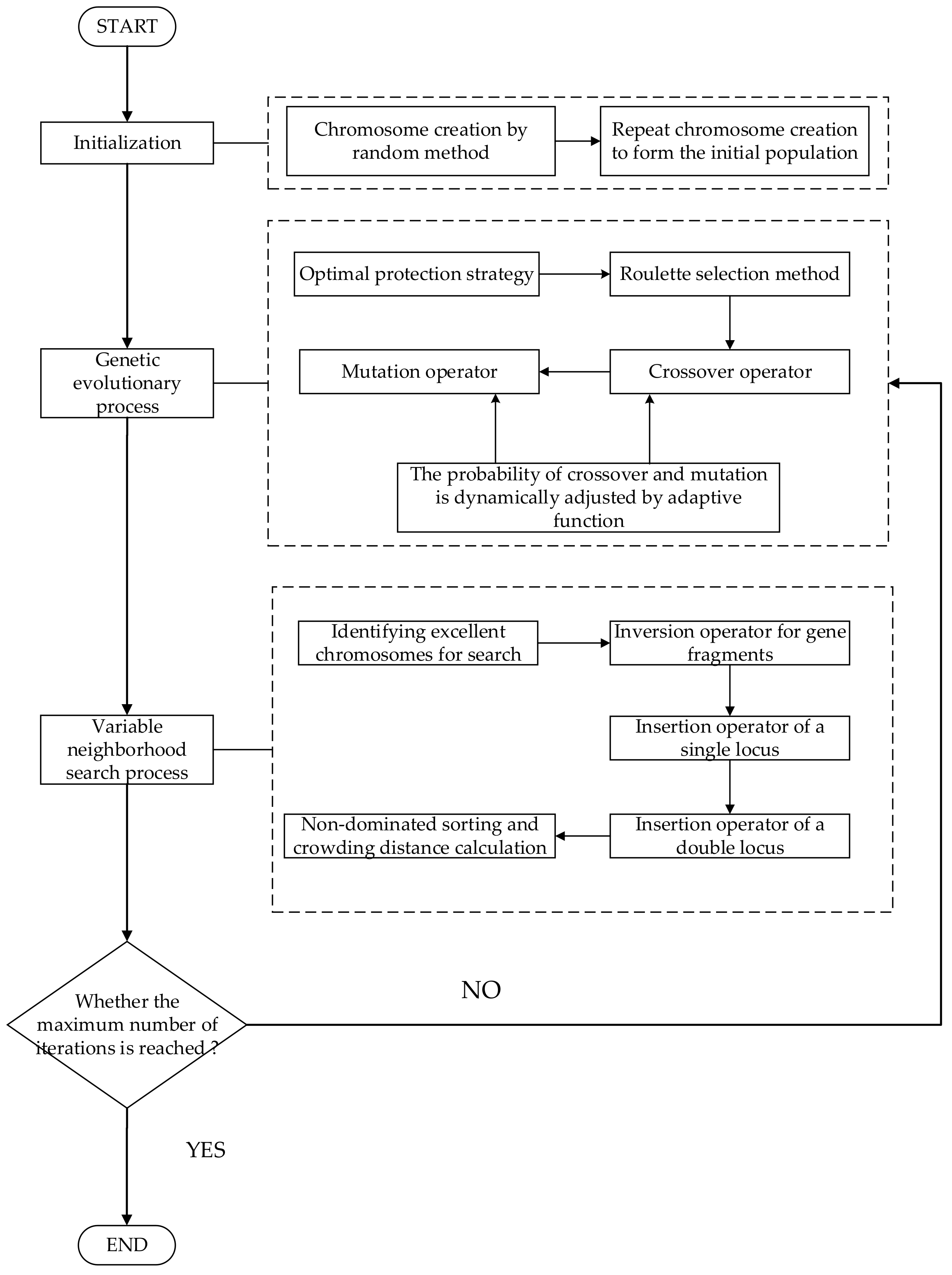
2.4. VNS-NSGA-II Algorithm
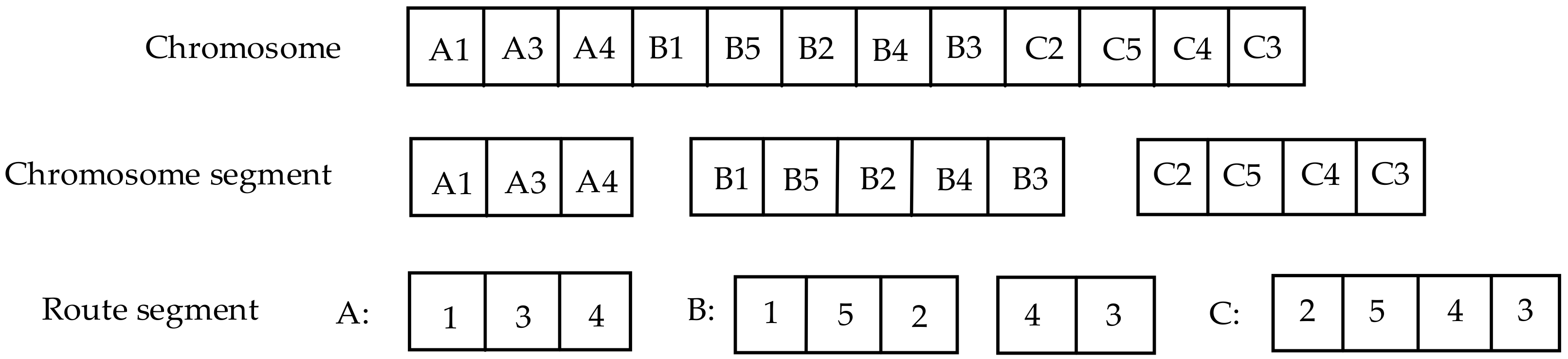
2.4.1. Population Initialization
2.4.2. Genetic Operator
- Selection Operator
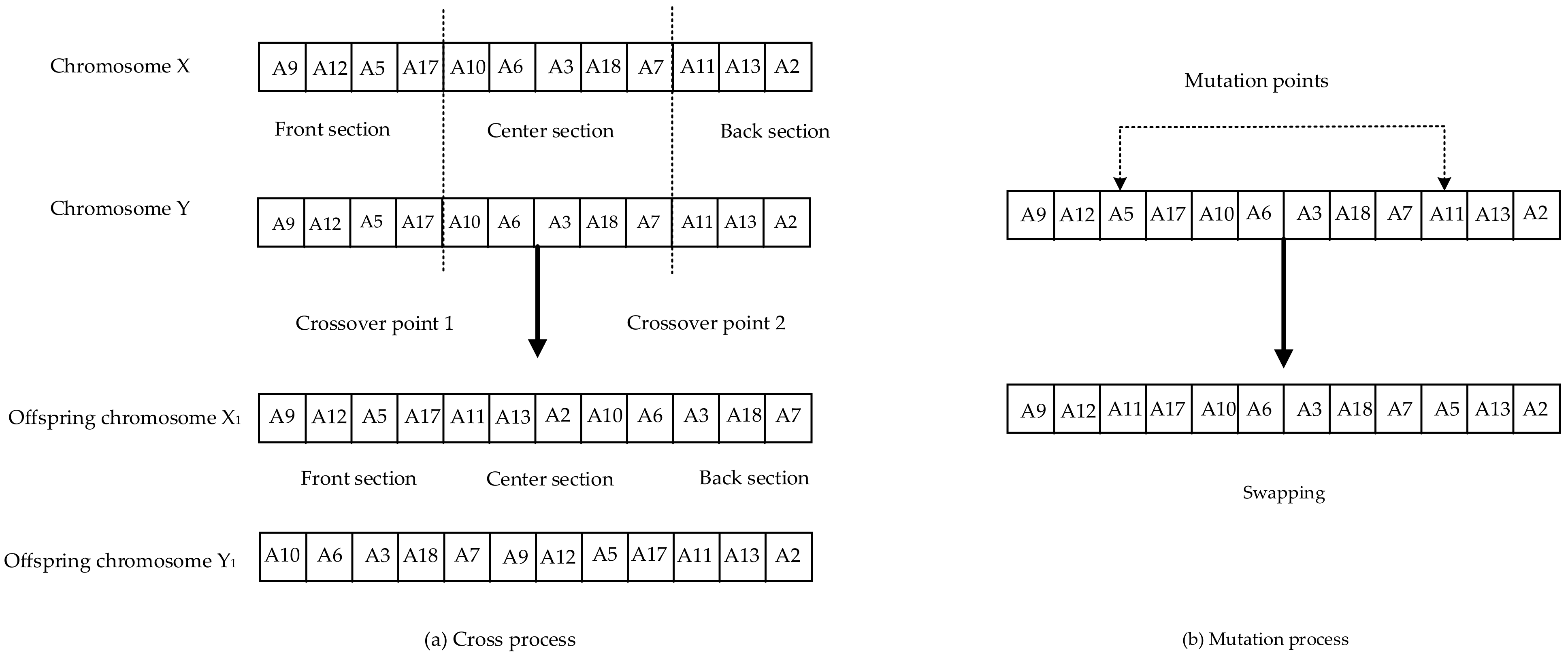
- Crossover Operator
- Mutation Operator
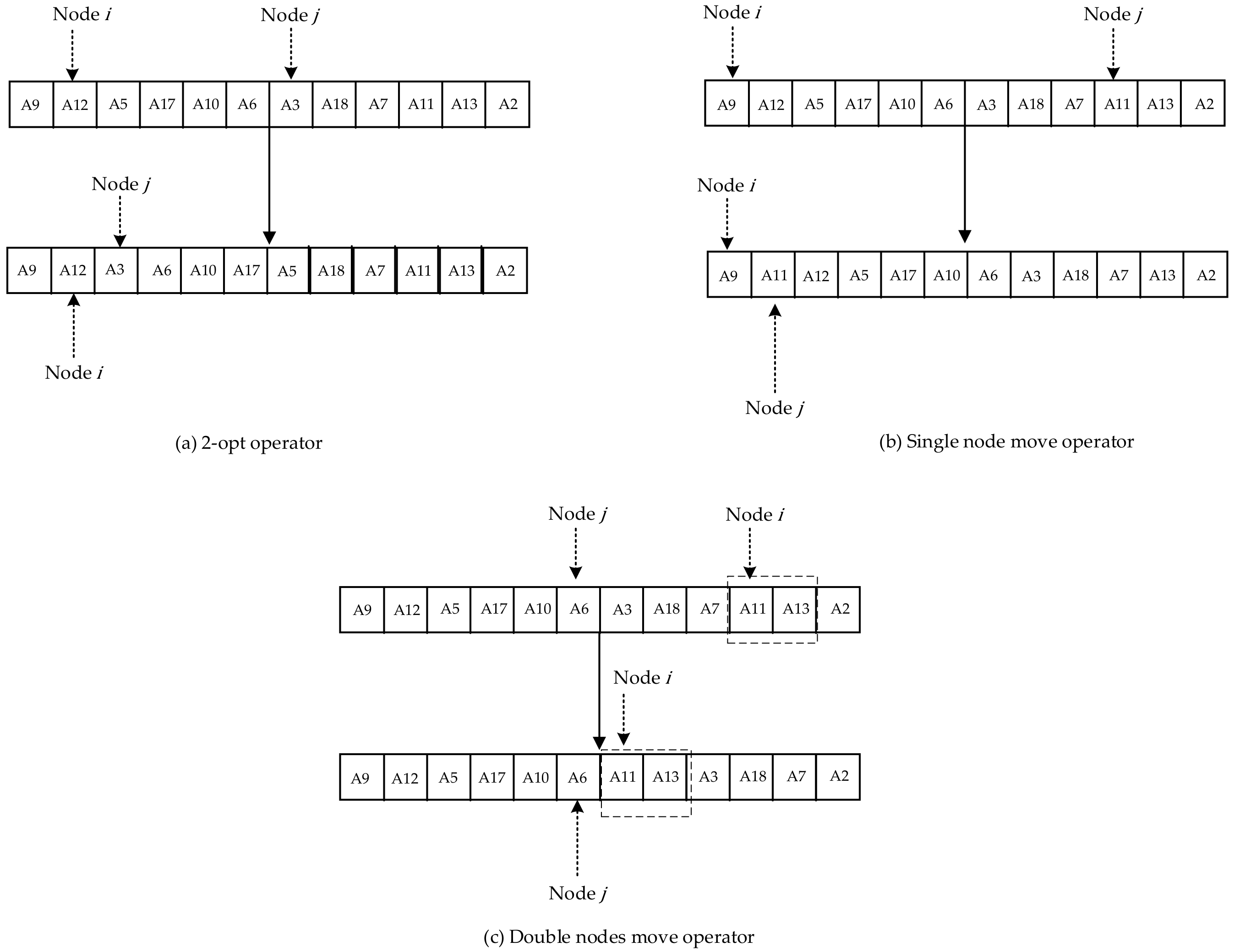
2.4.3. Variable Neighborhood Search Operators
- 2-opt operator
- Single node move operator
- Double nodes move operator
2.4.4. Non-Dominated Sorting and Crowding Distance Calculation
2.5. Select the Optimal Solution Strategy
2.6. Validation of the Simulation Model
3. Results and Discussion
3.1. Comparison with Other Efficient Algorithms
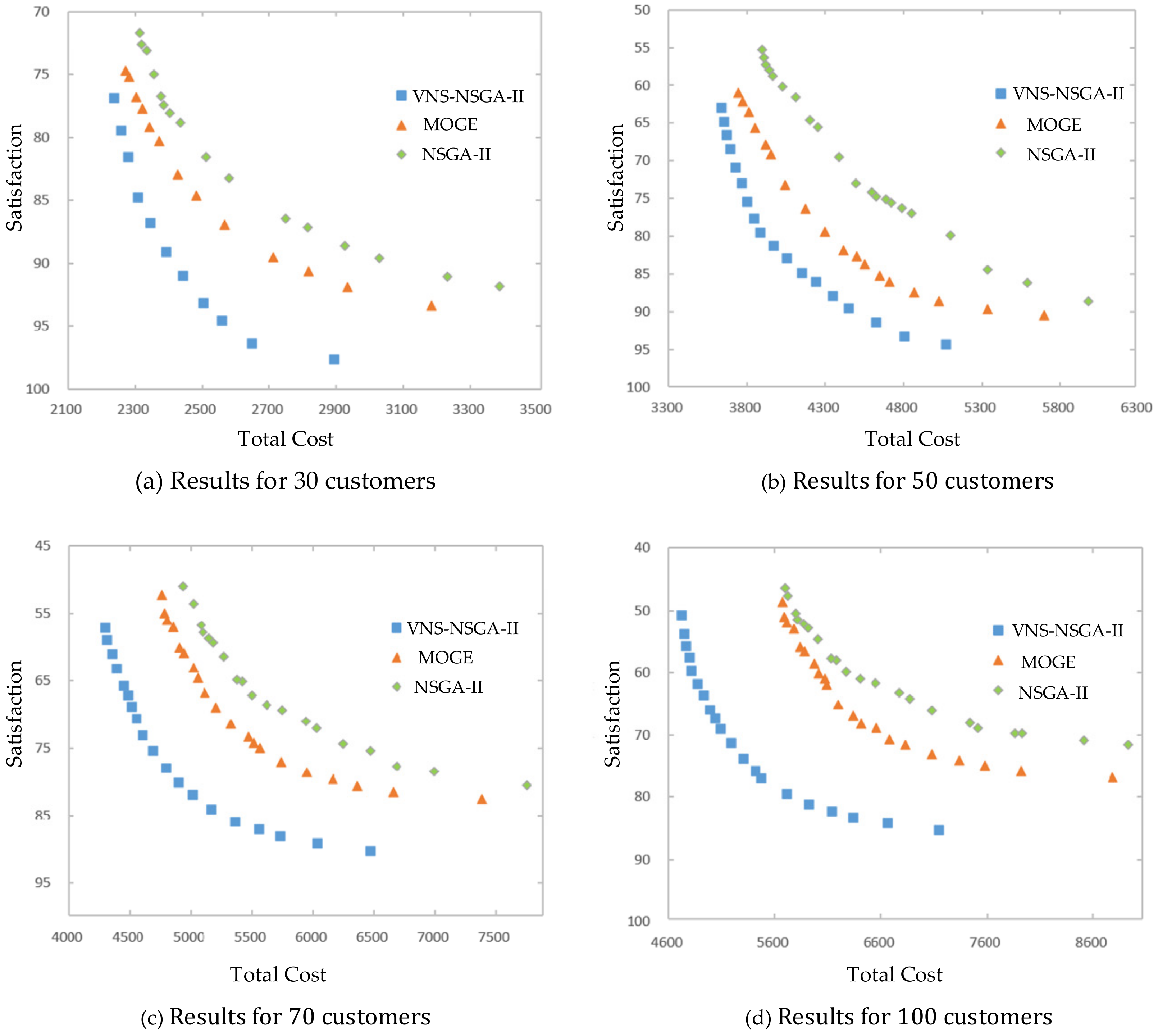
- (1)
- Comparison of Pareto-optimal fronts
- The VNS-NSGA-II algorithm is adaptive to the probability of crossover and mutation, which means that it can adjust the probability of crossover and mutation dynamically based on fitness, evolutionary algebra and the number of unchanged individuals during the evolution process, thereby minimizing the destruction of good solutions and ensuring population diversity. The adaptive function enhances the algorithm’s search capability and prevents premature convergence.
- The variable neighborhood search operators in VNS-NSGA-II reduce the possibility of the algorithm falling into the local optimum. Three mature neighborhood structures in variable neighborhood search operators increase the diversity of neighborhood space. The neighborhood space diversity is proportional to the offspring diversity. Greater neighborhood space diversity also represents the easier identification of the global optimal solution [47].
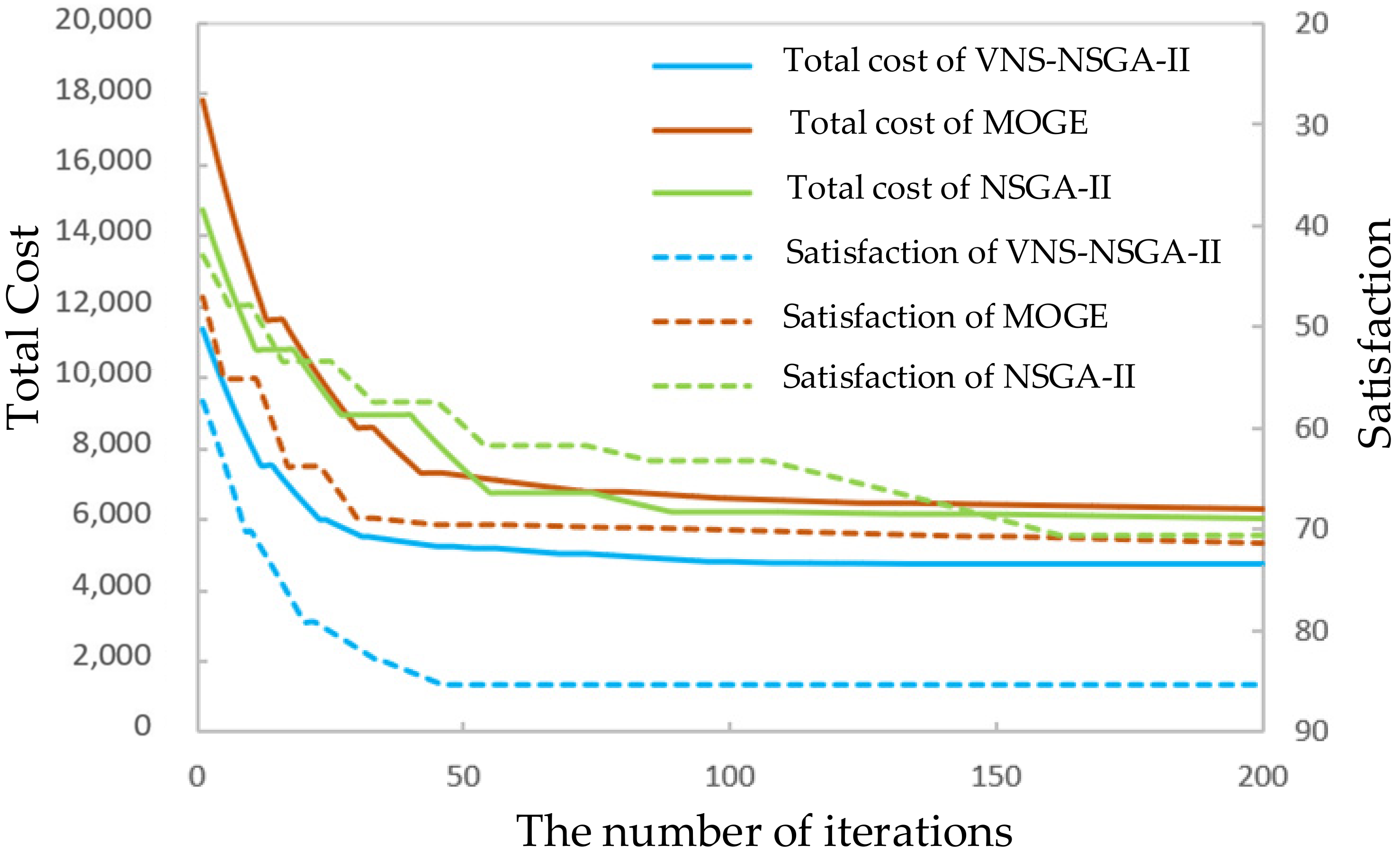
- (2)
- Comparison of convergence
3.2. Analysis of Optimal Solution Selection
3.3. Optimisation of the Fresh Agricultural Products Distribution Routes for the e-Commerce Business in the Sample
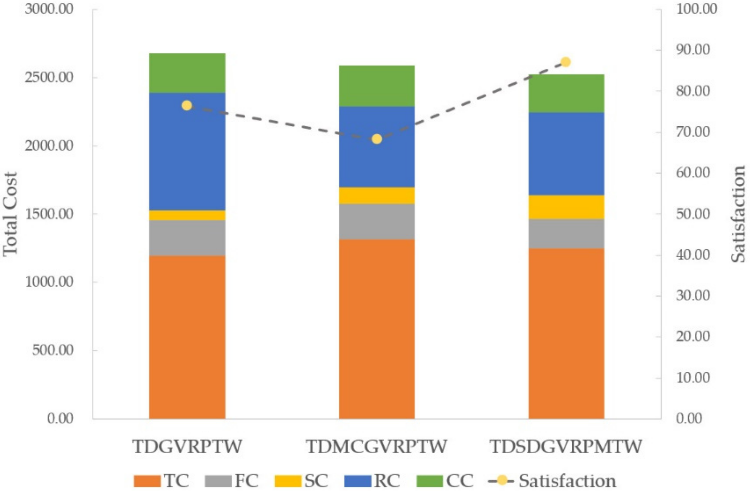
- Split delivery would allow customers ordering multiple agricultural products to be served by multiple vehicles, meaning that each vehicle would serve more customers and travel longer routes, which leads to higher travel costs and service costs. However, split delivery keeps each product at the optimum temperature for transport, which greatly reduces refrigeration costs and lowers the total cost.
- Split delivery allows each vehicle to deliver a smaller number of products to customers, which leads to a shorter service time that makes the vehicle more likely to finish each delivery and leave the customer within the optimal service time window, resulting in higher customer satisfaction. Another reason for the high level of satisfaction is that TDSDGVRPMTW chooses to refuse orders with products of small quantity and prioritizes serving customers ordering products of large quantity.
- Divide a vehicle’s compartment into multiple sections. Each of them transports one type of agricultural product with different optimum temperatures as needed. Although this can reduce refrigeration costs, if a customer’s demand for a certain type of agricultural product exceeds the capacity of the divided compartment, multiple deliveries are required to meet the customer’s demand for this type of agricultural product and more vehicles are needed, leading to high travel costs and carbon emissions.
- Customers have multiple time windows to choose and therefore vehicles have more opportunities to arrive at locations and complete services during a certain time window. The advantages of multiple time windows over a single time window will be leveraged, especially when a customer needs to be served by vehicles multiple times. One customer in TDMCGVRPTW needs the service of multiple vehicles, however, each customer has only one time window, and consequently many vehicles arrive at the location of the customer out of the time window, leading to very low customer satisfaction. Another reason for the low satisfaction is that TDMCGVRPTW chooses to refuse many orders for items that are in high demand, leaving many customers unserved.
- Therefore, the number of vehicle compartments, the capacity of each compartment, and the number of product types demanded by customers are the factors that determine why TDMCGVRPTW chooses not to deliver products that are in high demand and TDSDGVRPMTW chooses the opposite. The compartment of the vehicle in TDMCGVRPTW is divided into four parts. When a customer’s demand for a certain product exceeds the compartment capacity, multiple vehicles are required to deliver the same product to that customer. When the number of vehicles needed to serve the customer exceeds the number of types of products the customer orders, the service cost is too high and the order will be refused by TDMCGVRPTW. Therefore, under this circumstance, the advantages of TDSDGVRPMTW over TDMCGVRPTW can be observed. In terms of product types, TDSDGVRPMTW needs fewer vehicles to complete the distribution to the customer with lower service costs, thus, this customer order will not be refused. When the number of such customers is large, TDSDGVRPMTW would naturally become the best strategy.
4. Conclusions
Author Contributions
Funding
Data Availability Statement
Conflicts of Interest
References
- iResearch Institute. Research Report on Fresh Food E-Commerce Industry in China. 2021. Available online: https://www.iresearch.com.cn/Detail/report?id=3776&isfree=0 (accessed on 7 April 2022).
- Hsu, C.; Chen, W. Optimizing fleet size and delivery scheduling for multi-temperature food distribution. Appl. Math. Model. 2014, 38, 1077–1091. [Google Scholar] [CrossRef]
- Reed, M.; Yiannakou, A.; Evering, R. An ant colony algorithm for the multi-compartment vehicle routing problem. Appl. Soft Comput. 2014, 15, 169–176. [Google Scholar] [CrossRef] [Green Version]
- Arora, R.; Kaushik, C.; Arora, R. Multi-objective and multi-parameter optimization of two-stage thermoelectric generator in electrically series and parallel configurations through NSGA-II. Energy 2015, 91, 242–254. [Google Scholar] [CrossRef]
- Osvald, A.; Stirn, L. A vehicle routing algorithm for the distribution of fresh vegetables and similar perishable food. J. Food Eng. 2008, 85, 285–295. [Google Scholar] [CrossRef]
- Wen, M.; Krapper, E.; Larsen, J.; Stidsen, T. A multilevel variable neighborhood search heuristic for a practical vehicle routing and driver scheduling problem. Networks 2011, 58, 311–322. [Google Scholar] [CrossRef] [Green Version]
- Stellingwerf, H.; Groeneveld, L.; Laporte, G.; Kanellopoulos, A.; Bloemhof, J.; Behdani, B. The quality-driven vehicle routing problem: Model and application to a case of cooperative logistics. Int. J. Prod. Econ. 2021, 231, 107849. [Google Scholar] [CrossRef]
- Yao, B.; Chen, C.; Song, X.; Yang, X. Fresh seafood delivery routing problem using an improved ant colony optimization. Ann. Oper. Res. 2019, 273, 163–186. [Google Scholar] [CrossRef]
- Zhao, Z.; Li, X.; Zhou, X. Optimization of transportation routing problem for fresh food in time-varying road network: Considering both food safety reliability and temperature control. PLoS ONE 2020, 15, e0235950. [Google Scholar] [CrossRef]
- Hsiao, Y.; Chen, M.; Lu, K.; Chin, C. Last-mile distribution planning for fruit-and-vegetable cold chains. Int. J. Logist. Manag. 2018, 29, 862–886. [Google Scholar] [CrossRef]
- Dror, M.; Trudeau, P. Split delivery routing. Nav. Res. Logist. NRL 1990, 37, 383–402. [Google Scholar] [CrossRef]
- Dror, M.; Trudeau, P. Savings by split delivery routing. Transp. Sci. 1989, 23, 141–145. [Google Scholar] [CrossRef]
- Ambrosino, D.; Sciomachen, A. A food distribution network problem: A case study. IMA J. Manag. Math. 2006, 18, 33–53. [Google Scholar] [CrossRef]
- Yoshizaki, H.T.Y. Scatter search for a real-life heterogeneous fleet vehicle routing problem with time windows and split deliveries in Brazil. Eur. J. Oper. Res. 2009, 199, 750–758. [Google Scholar]
- Wu, D.; Wu, C. TDGVRPSTW of fresh agricultural products distribution: Considering both economic cost and environmental cost. Appl. Sci. 2021, 11, 10579. [Google Scholar] [CrossRef]
- Frizzell, W.; Giffin, W. The split delivery vehicle scheduling problem with time windows and grid network distances. Comput. Oper. Res. 1995, 22, 655–667. [Google Scholar] [CrossRef]
- Silva, M.; Subramanian, A.; Ochi, S. An iterated local search heuristic for the split delivery vehicle routing problem. Comput. Oper. Res. 2015, 53, 234–249. [Google Scholar] [CrossRef]
- Yang, W.; Wang, D.; Pang, W.; Tan, A.; Zhou, Y. Goods consumed during transit in split delivery vehicle routing problems: Modeling and solution. IEEE Access 2020, 8, 110336–110350. [Google Scholar] [CrossRef]
- Sin, C.; Haugland, D. A tabu search heuristic for the vehicle routing problem with time windows and split deliveries. Comput. Oper. Res. 2004, 31, 1947–1964. [Google Scholar]
- Desaulniers, G. Branch-and-price-and-cut for the split-delivery vehicle routing problem with time windows. Oper. Res. 2010, 58, 179–192. [Google Scholar] [CrossRef]
- Archetti, C.; Bouchard, M.; Desaulniers, G. Enhanced branch and price and cut for vehicle routing with split deliveries and time windows. Transp. Sci. 2011, 45, 285–298. [Google Scholar] [CrossRef]
- Salani, M.; Vacca, I. Branch and price for the vehicle routing problem with discrete split deliveries and time windows. Eur. J. Oper. Res. 2011, 213, 470–477. [Google Scholar] [CrossRef] [Green Version]
- Bianchessi, N.; Irnich, S. Branch-and-cut for the split delivery vehicle routing problem with time windows. Transp. Sci. 2019, 53, 442–462. [Google Scholar] [CrossRef] [Green Version]
- Luo, Z.; Qin, H.; Zhu, W.; Lim, A. Branch and price and cut for the split-delivery vehicle routing problem with time windows and linear weight-related cost. Transp. Sci. 2017, 51, 668–687. [Google Scholar] [CrossRef]
- McNabb, E.; Weir, D.; Hill, R.; Hall, S. Testing local search move operators on the vehicle routing problem with split deliveries and time windows. Comput. Oper. Res. 2015, 56, 93–109. [Google Scholar] [CrossRef]
- Li, J.; Qin, H.; Baldacci, R.; Zhu, W. Branch-and-price-and-cut for the synchronized vehicle routing problem with split delivery, proportional service time and multiple time windows. Transp. Res. Part E Logist. Transp. Rev. 2020, 140, 101955. [Google Scholar] [CrossRef]
- Wang, H.; Du, L.; Ma, S. Multi-objective open location-routing model with split delivery for optimized relief distribution in post-earthquake. Transp. Res. Part E Logist. Transp. Rev. 2014, 69, 160–179. [Google Scholar] [CrossRef]
- Vahdani, B.; Veysmoradi, D.; Noori, F.; Mansour, F. Two-stage multi-objective location-routing-inventory model for humanitarian logistics network design under uncertainty. Int. J. Disaster Risk Reduct. 2018, 27, 290–306. [Google Scholar] [CrossRef]
- Goodarzi, H.; Tavakkoli-Moghaddam, R.; Amini, A. A new bi-objective vehicle routing-scheduling problem with cross-docking: Mathematical model and algorithms. Comput. Ind. Eng. 2020, 149, 106832. [Google Scholar] [CrossRef]
- Hickman, A.; Hassel, D.; Joumard, R. Methodology for Calculating Transport Emissions and Energy Consumption; The National Academies of Sciences, Engineering, and Medicine: Washington, DC, USA, 1999; pp. 1–362. [Google Scholar]
- Malandraki, C.; Daskin, M. Time dependent vehicle routing problems: Formulations, properties and heuristic algorithms. Transp. Sci. 1992, 26, 185–200. [Google Scholar] [CrossRef]
- Malandraki, C.; Dial, B. A restricted dynamic programming heuristic algorithm for the time dependent traveling salesman problem. Eur. J. Oper. Res. 1996, 90, 45–55. [Google Scholar] [CrossRef]
- Ichoua, S.; Gendreau, M.; Potvin, J. Vehicle dispatching with time-dependent travel times. Eur. J. Oper. Res. 2003, 144, 379–396. [Google Scholar] [CrossRef] [Green Version]
- Fleischmann, B.; Gietz, M.; Gnutzmann, S. Time-varying travel times in vehicle routing. Transp. Sci. 2004, 38, 160–173. [Google Scholar] [CrossRef]
- Wang, Y.; Zhang, J.; Guan, X.; Xu, M.; Wang, Z.; Wang, H. Collaborative multiple centers fresh logistics distribution network optimization with resource sharing and temperature control constraints. Expert Syst. Appl. 2021, 165, 113838. [Google Scholar] [CrossRef]
- Wang, X.; Wang, M.; Ruan, J.; Li, Y. Multi-objective optimization for delivering perishable products with mixed time windows. Adv. Prod. Eng. Manag. 2018, 13, 321–332. [Google Scholar] [CrossRef] [Green Version]
- Wang, H.; Li, W.; Zhao, Z.; Wang, Z.; Li, M.; Li, D. Intelligent distribution of fresh agricultural products in smart city. IEEE Trans. Ind. Inform. 2021, 18, 1220–1230. [Google Scholar] [CrossRef]
- Xu, H.; Fan, W.; Wei, T.; Yu, L. An Or-opt NSGA-II algorithm for multi-objective vehicle routing problem with time windows. In Proceedings of the 2008 IEEE International Conference on Automation Science and Engineering, Arlington, VA, USA, 23 August 2008; pp. 309–314. [Google Scholar]
- Wang, Y.; Zhang, S.; Guan, X.; Peng, S.; Wang, H.; Liu, Y.; Xu, M. Collaborative multi-depot logistics network design with time window assignment. Expert Syst. Appl. 2020, 140, 112910. [Google Scholar] [CrossRef]
- Wang, Y.; Zhang, J.; Assogba, K.; Liu, Y.; Xu, M.; Wang, Y. Collaboration and transportation resource sharing in multiple centers vehicle routing optimization with delivery and pickup. Knowl. Based Syst. 2018, 160, 296–310. [Google Scholar] [CrossRef]
- Pacciarelli, D.; Løkketangen, A.; Mandal, K.; Hasle, G. A memetic NSGA-II for the bi-objective mixed capacitated general routing problem. J. Heuristics 2015, 21, 359–390. [Google Scholar]
- Fan, H.; Zhang, Y.G.; Tian, P.J.; Cao, Y.; Ren, X.X. Dynamic vehicle routing problem of heterogeneous fleets with time-dependent networks. Syst. Eng. Theory Pract. 2022, 42, 455–470, (In Chinese with English Abstract). [Google Scholar] [CrossRef]
- Sánchez-Oro, J.; López-Sánchez, A.D.; Colmenar, J.M. A general variable neighborhood search for solving the multi-objective open vehicle routing problem. J. Heuristics 2020, 26, 423–452. [Google Scholar] [CrossRef]
- Solomon, M.M. Algorithms for the vehicle routing and scheduling problems with time window constraints. Oper. Res. 1987, 35, 254–265. [Google Scholar] [CrossRef] [Green Version]
- Liu, C.; Kou, G.; Zhou, X.; Peng, Y.; Sheng, H.; Alsaadi, F.E. Time-dependent vehicle routing problem with time windows of city logistics with a congestion avoidance approach. Knowl. Based Syst. 2019, 188, 104813. [Google Scholar] [CrossRef]
- Zulvia, E.; Kuo, J.; Nugroho, Y. A many-objective gradient evolution algorithm for solving a green vehicle routing problem with time windows and time dependency for perishable products. J. Clean Prod. 2020, 242, 118428. [Google Scholar] [CrossRef]
- Jiang, Z.; Chen, Y.; Li, X.; Li, B. A heuristic optimization approach for multi-vehicle and one-cargo green transportation scheduling in shipbuilding. Adv. Eng. Inform. 2021, 49, 101306. [Google Scholar] [CrossRef]


| Variable | Definition | Parameter | Definition | Set | Definition |
|---|---|---|---|---|---|
| The cost of the vehicle’s travel | The number of customers that need to be delivered | Set of all nodes in the distribution network, including the distribution center and all customer points | |||
| The cost of vehicle’s fixed use | The vehicle’s travel cost per unit distance | ||||
| The cost of customer service | The fixed cost per vehicle | Set of all vehicles | |||
| The cost of refrigeration | Set of all time periods | ||||
| The cost of carbon emissions | The maximum capacity of the vehicle | Set of all types of fresh agricultural products | |||
| Maximum number of vehicles that can be used | |||||
| in the logistics distribution network | for various fresh agricultural products | ||||
| . | |||||
| to receive service | |||||
| to receive service | |||||
| . | |||||
| , and 0 otherwise | |||||
| , and 0 otherwise | |||||
| , and 0 otherwise | |||||
| is used, and 0 otherwise |
| Number of Customers | Number of Vehicles | Total Demand | Type of Agricultural Products | Unit Price of Agricultural Products |
|---|---|---|---|---|
| 30 | 8 | 520 | A | 10 |
| B | 12 | |||
| 50 | 15 | 860 | A | 10 |
| B | 12 | |||
| 70 | 20 | 1210 | A | 10 |
| B | 12 | |||
| C | 15 | |||
| D | 20 | |||
| 100 | 25 | 1810 | A | 10 |
| B | 12 | |||
| C | 15 | |||
| D | 20 |
| Number of Customers | Total Demand | VNS-NSGA-II | NSGA-II | MOGE | Compared with NSGA-II | Compared with MOGE | |||||
|---|---|---|---|---|---|---|---|---|---|---|---|
| TTC | Satisfaction | TTC | Satisfaction | TTC | Satisfaction | TTC Reduction % | Satisfaction Increases | TTC Reduction % | Satisfaction Increases | ||
| 30 | 520 | 2212.50 | 96.64 | 2301.80 | 90.36 | 2260.71 | 91.86 | 3.88% | 6.28 | 2.13% | 4.79 |
| 50 | 860 | 3608.27 | 93.44 | 3844.34 | 87.57 | 3681.60 | 88.77 | 6.14% | 5.87 | 1.99% | 4.66 |
| 70 | 1210 | 4246.75 | 88.44 | 4865.36 | 79.52 | 4687.99 | 80.96 | 12.71% | 8.92 | 9.41% | 7.49 |
| 100 | 1810 | 4689.05 | 84.51 | 5674.60 | 70.48 | 5642.77 | 75.51 | 17.37% | 14.03 | 16.90% | 8.99 |
| Mean | 1100 | 3689.14 | 90.76 | 4171.52 | 81.98 | 4068.27 | 84.27 | 10.03% | 8.77 | 7.61% | 6.48 |
| No. | TTC | Satisfaction | |||
|---|---|---|---|---|---|
| 1 | 7159.35 | 85.33 | 0.15324 | 0.07745 | 0.33572 |
| 2 | 6669.93 | 84.23 | 0.14917 | 0.06207 | 0.29384 |
| 3 | 6339.67 | 83.36 | 0.14683 | 0.05212 | 0.26196 |
| 4 | 6132.93 | 82.36 | 0.14382 | 0.04670 | 0.24512 |
| 5 | 5916.87 | 81.31 | 0.14107 | 0.04191 | 0.22905 |
| 6 | 5720.60 | 79.56 | 0.13560 | 0.04074 | 0.23101 |
| 7 | 5470.51 | 76.94 | 0.12784 | 0.04415 | 0.25670 |
| 8 | 5413.11 | 75.86 | 0.12433 | 0.04738 | 0.27591 |
| 9 | 5304.79 | 73.74 | 0.11767 | 0.05464 | 0.31709 |
| 10 | 5176.35 | 71.30 | 0.11072 | 0.06388 | 0.36585 |
| 11 | 5083.69 | 69.12 | 0.10476 | 0.07280 | 0.41003 |
| 12 | 5029.63 | 67.43 | 0.10022 | 0.07997 | 0.44381 |
| 13 | 4990.14 | 65.90 | 0.09622 | 0.08657 | 0.47360 |
| 14 | 4924.46 | 63.60 | 0.09103 | 0.09657 | 0.51477 |
| 15 | 4877.52 | 61.75 | 0.08737 | 0.10469 | 0.54507 |
| 16 | 4813.10 | 59.75 | 0.08457 | 0.11347 | 0.57296 |
| 17 | 4787.05 | 57.70 | 0.08147 | 0.12251 | 0.60062 |
| 18 | 4770.79 | 55.69 | 0.07903 | 0.13145 | 0.62454 |
| 19 | 4755.34 | 53.77 | 0.07760 | 0.13995 | 0.64331 |
| 20 | 4724.00 | 50.77 | 0.07745 | 0.15324 | 0.66428 |
| No. | TTC | CC | RC | Number of Vehicles Used | Average Loading Rate | Satisfaction |
|---|---|---|---|---|---|---|
| 1 | 7159.35 | 11.65% | 34.13% | 22 | 43.67% | 85.33 |
| 5 | 5916.87 | 7.79% | 26.46% | 15 | 59.72% | 81.31 |
| 20 | 4724.00 | 5.83% | 16.51% | 12 | 74.92% | 50.77 |
| No. | X | Y | Demand (kg) | Ready Time | Due Time | Types |
|---|---|---|---|---|---|---|
| 0 | 31 | 47 | 0 | 5:00 | 17:30 | |
| 1 | 37 | 61 | 500 | 6:30 | 8:30 | A, B |
| 2 | 31 | 29 | 350 | 5:30 | 8:30 | A |
| 3 | 51 | 57 | 600 | 6:00 | 9:00 | A |
| 4 | 51 | 32 | 900 | 12:00 | 15:00 | B, C |
| 5 | 11 | 42 | 1200 | 8:00 | 12:00 | A, D |
| 6 | 21 | 42 | 100 | 15:00 | 16:00 | B |
| 7 | 16 | 62 | 250 | 6:00 | 11:00 | A, C |
| 8 | 6 | 55 | 400 | 7:30 | 10:00 | A, B |
| 9 | 51 | 72 | 800 | 9:00 | 10:30 | C |
| 10 | 26 | 72 | 750 | 11:00 | 11:30 | B |
| 11 | 16 | 77 | 600 | 7:30 | 9:30 | D |
| 12 | 46 | 47 | 800 | 6:00 | 8:00 | A, C |
| 13 | 26 | 37 | 1150 | 10:00 | 11:30 | B, D |
| 14 | 11 | 22 | 1000 | 5:00 | 7:00 | A, C |
| 15 | 26 | 17 | 400 | 14:30 | 16:30 | A, D |
| 16 | 6 | 32 | 900 | 5:30 | 7:00 | C |
| 17 | 1 | 42 | 150 | 6:00 | 8:00 | A |
| 18 | 16 | 52 | 500 | 7:00 | 8:30 | D |
| 19 | 11 | 72 | 800 | 6:30 | 8:00 | B, C |
| 20 | 41 | 77 | 450 | 8:30 | 9:30 | A |
| 21 | 41 | 32 | 500 | 7:30 | 10:30 | B, C |
| 22 | 41 | 22 | 850 | 13:00 | 14:30 | A |
| 23 | 51 | 17 | 1450 | 7:00 | 12:00 | A, D |
| 24 | 61 | 47 | 150 | 9:00 | 11:30 | B |
| TTC | TC | FC | SC | RC | CC | Satisfaction | |
|---|---|---|---|---|---|---|---|
| TDGVRPTW | 2680.95 | 1194.32 | 260.00 | 72.00 | 861.88 | 292.75 | 76.36 |
| TDMCGVRPTW | 2587.27 | 1317.44 | 260.00 | 117.00 | 594.55 | 298.28 | 68.15 |
| TDSDGVRPMTW | 2525.17 | 1246.67 | 220.00 | 174.00 | 603.89 | 280.60 | 87.04 |
| Gap_mc | −93.68 | 123.12 | 0.00 | 45.00 | −267.33 | 5.53 | −8.21 |
| Gap_sd | −155.78 | 52.35 | −40.00 | 102.00 | −257.98 | −12.15 | 10.68 |
| A | B | C | D | |||||
|---|---|---|---|---|---|---|---|---|
| PD | Proportion | PD | Proportion | PD | Proportion | PD | Proportion | |
| TDGVRPTW | 4450 | 78.21% | 3060 | 71.66% | 2795 | 75.95% | 1245 | 65.18% |
| TDMCGVRPTW | 3525 | 61.95% | 2730 | 63.93% | 2645 | 71.88% | 1435 | 75.13% |
| TDSDGVRPMTW | 5290 | 92.97% | 3770 | 88.29% | 3020 | 82.07% | 1375 | 71.99% |
| Refrigeration cost per minute | 0.65 | 0.68 | 1.02 | 1.13 | ||||
| Total Demand | 5690 | 4270 | 3680 | 1910 | ||||
Publisher’s Note: MDPI stays neutral with regard to jurisdictional claims in published maps and institutional affiliations. |
© 2022 by the authors. Licensee MDPI, Basel, Switzerland. This article is an open access article distributed under the terms and conditions of the Creative Commons Attribution (CC BY) license (https://creativecommons.org/licenses/by/4.0/).
Share and Cite
Wu, D.; Wu, C. Research on the Time-Dependent Split Delivery Green Vehicle Routing Problem for Fresh Agricultural Products with Multiple Time Windows. Agriculture 2022, 12, 793. https://doi.org/10.3390/agriculture12060793
Wu D, Wu C. Research on the Time-Dependent Split Delivery Green Vehicle Routing Problem for Fresh Agricultural Products with Multiple Time Windows. Agriculture. 2022; 12(6):793. https://doi.org/10.3390/agriculture12060793
Chicago/Turabian StyleWu, Daqing, and Chenxiang Wu. 2022. "Research on the Time-Dependent Split Delivery Green Vehicle Routing Problem for Fresh Agricultural Products with Multiple Time Windows" Agriculture 12, no. 6: 793. https://doi.org/10.3390/agriculture12060793