A 1D-SP-Net to Determine Early Drought Stress Status of Tomato (Solanum lycopersicum) with Imbalanced Vis/NIR Spectroscopy Data

Abstract

Detection of the early stages of stress is crucial in stabilizing crop yields and agricultural production. The aim of this study was to construct a nondestructive and robust method to predict the early physiological drought status of the tomato (Solanum lycopersicum); for this purpose, a convolutional neural network (CNN)-based model with a one-dimensional (1D) kernel for fitting the visible and near infrared (Vis/NIR) spectral data was proposed. To prevent degradation and enhance the feature comprehension of the deep neural network architecture, residual and global context modules were embedded in the proposed 1D-CNN model, yielding the 1D spectrogram power net (1D-SP-Net). The 1D-SP-Net outperformed the 1D-CNN, partial least squares discriminant analysis (PLSDA), and random forest (RF) models in model testing, demonstrating an accuracy of 96.3%, precision of 98.0%, Matthew’s correlation coefficient of 0.92, and an F1 score of 0.95. Furthermore, when employing various synthesized imbalanced data sets, the proposed 1D-SP-Net remained robust and consistent, outperforming the other models in terms of the prediction capabilities. These results indicate that the 1D-SP-Net is a promising model resistant to the effects of imbalanced data sets and able to determine the early drought stress status of tomato seedlings in a non-invasive manner.

1. Introduction

Crop growth and yield are subject to both biotic and abiotic environmental factors. Due to ongoing severe climate change, these factors frequently exceed critical levels and induce various types of plant stress [1]. The major goal of agricultural research is to overcome such adverse impacts and to enhance crop productivity under diverse conditions of stress. Present solutions for the reduction of the adverse effects caused by stress mainly rely on crop breeding and management methods. Breeding crops to exhibit certain stress tolerances or resistance characteristics requires years and also sufficient prior genetic and phenotypic knowledge [2,3]. By contrast, the implementation of proper management before the occurrence of irreversible damage and yield loss is both efficient and effective [4]. However, both solutions require deep understanding of the progression of stress induction, for which methodologies capable of detecting stress responses in the early stages are essential [5,6]. Those methodologies include the determination of specific gene expression by polymerase chain reaction technology, quantification of enzyme activity and of active compounds by zymography, spectrometry, and chromatography analysis, and the direct or indirect measurement of other physiological parameters by various technologies and methods [7,8,9,10,11]. Nevertheless, these methods are relatively invasive, time-consuming, and poorly replicable. The development of nondestructive, rapid, and high-volume remote sensing technique is a promising option for the detection of plant disease and stress [12,13].

Remote sensing technique can provide timely, cost-effective, and reliable information of the instant alteration of plant physiology. Among various type of remote sensing techniques, the visible and near infrared (Vis/NIR) spectroscopy that covers the reflectance radiation regions of electromagnetic spectrum of 400–700 nm and 700–1200 nm are significantly correlated with the physiological status, pigmentation, and cell structure [14,15,16]. To establish a prediction model that links the spectral data to certain characteristics of interest is a goal being pursued in the fields of pharmaceutical, environmental, food science, and agricultural research [17,18,19,20]. In the field of agricultural research, Vis/NIR spectral data have been used extensively to construct predictive models for the determination of plant diseases and abiotic stress [21,22]. The accurate detection of water stress in the early stage for tomato (Solanum lycopersicum), lettuce (Lactuca sativa), and grapevine (Vitis spp.) are possible through the use of Vis/NIR spectroscopy [23,24,25]. Reflectance spectral data of Vis/NIR are used to calculate vegetation indices that are capable of remotely sensing physiological responses of water and salinity stress in rice (Oryza sativa), tomato, and potato (Solanum tuberosum) [20,26,27]. Furthermore, Sanseechan et al. [28] successfully implemented a measurement method by NIR spectroscopy to estimate the solid density of cane stake in a sugarcane breeding program. The ability to provide dynamic spectra over time and space makes the Vis/NIR spectroscopy a potential real-time monitoring tool for plant growth and quality [29,30].

Among abiotic stresses, drought is one of the most stringent and can prompt a transition in physiological status from normal to under stress within days and leads to abnormal growth gradually and eventual wilting [31,32]. In the early stages of drought stress, physiological status transition is commonly revealed as invisible alterations in leaf anatomy, biochemistry composition, and activities in the photosynthesis system II (PSII) that contribute to decline in leaf stomatal conductance and transpiration rate [33]. Those early invisible alterations can be captured by the Vis/NIR spectroscopy and result in variations in the leaf reflectance spectrum [26,27]. However, before informative spectral data can be used for model construction, certain factors must be resolved. Intrinsic high dimensionality and the high correlation between neighboring wavelengths of spectral data can complicate the modeling process and must be addressed prior to initiating such a process [34]. Partial least squares regression (PLSR) and partial least squares discriminant analysis (PLSDA) are techniques capable of reducing high dimensionality and resolving the collinearity commonly applied to connect spectral data with specific plant physiological responses [14,15,20,25,35]. Although partial least squares (PLS)-based models are powerful tools for specifically addressing collinearity, potential model overfitting may occur occasionally because of the inappropriate selection of tunable latent variables (LVs) [36,37].

An alternative to PLS-based statistical methods, machine learning models such as random forests (RFs) and convolutional neural networks (CNNs) are other options for analyzing spectral data [38,39]. RF is a powerful classifier that can integrate numerous single classification and regression trees (CART) and can introduce random procedures for model training. RF retains the classification and regression capabilities of CART, exhibits greater robustness than a single CART, and also reduces the occurrence of overfitting [40]. CNNs are a class of feed-forward neural network with shared and learnable weights architectures [41]. CNNs have been applied extensively in image recognition, natural language processing, and medical diagnosis because of their outstanding capabilities in feature extraction and dimension reduction without the loss of data characteristics [42,43,44]. In addition to two-dimensional (2D) and three-dimensional (3D) structured data, CNNs have already been successfully applied to various one-dimensional (1D) structured data, including bio-signals for biomedical applications and vibration spectroscopy in agricultural research [45,46]. Acquarelli et al. [45] proposed a 1D-CNN to analyze NIR spectral data and demonstrated that the 1D-CNN was less affected by data preprocessing than PLSDA. A proper preprocessing for NIR spectral data is a key step but no formal or standardized rules have been established. These advantages indicate that CNNs are a promising option for qualitative and quantitative analysis of NIR spectroscopy [46].

In real-word classification problems, the inevitable difficulty is the occurrence of imbalanced data sets in which the sample sizes of different classes are distributed unequally, which is especially true for data sets obtained from biological trials [47]. A class-imbalance data set often causes unpredictable reductions in model performance [48]. A common approach to mitigate the effects of class-imbalance data sets on model performance is to reweight the skewed class distribution in the training data set through diverse sampling methods [47,48]. Nevertheless, the synthetic training data set may be entirely distinct from the original data set; thus, even more severely biased data distribution may be introduced [48]. Another remedy relies on the selection of an adequate and robust model that is influenced to a lesser degree by an imbalanced data set [49]. To address factors related to class imbalance, several algorithms that use CNN-based models coupled with cost-sensitive, output thresholding, and extremely deep neural network strategies have been proposed [50,51,52]. Khan et al. [53] reported that the cost-sensitive CNN outperformed the RF and sampling methods with class-imbalanced data sets. However, gradient exploding or vanishing and degradation problems may arise in the deep architecture of the neural network in CNN-based models, and this may impede the model training process and reduce the performance of the CNN model [54,55]. He et al. [56] proposed a residual learning module to mitigate the negative effect of gradient exploding or vanishing and degradation. Furthermore, a global context (GC) module that combines nonlocal and squeeze-and-excitation learning was demonstrated to enhance feature comprehension and to lower computation expenditure [57]. These modules can be embedded in a CNN model and relieve the adverse effects that arise from the deep architecture of neural networks.

To the best of our knowledge, CNN-based models for the discrimination of normal and stress physiological status in the tomato plant have seldom been researched. The aim of this study was to construct a nondestructive prediction method for determining the physiological drought status in its early stage for the “Rosada” tomato variety. To address the adverse effects on model performance due to imbalanced data structures, a CNN model with a 1D kernel to fit the NIR reflectance spectral data was established. In addition, residual and GC blocks were embedded in the proposed 1D-CNN to prevent degradation and to enhance feature comprehension. The 1D-CNN embedded with residual and GC blocks, the 1D spectrogram power net (1D-SP-Net) was further compared with the 1D-CNN, regular PLSDA, and RF models to evaluate its prediction performance. Moreover, various imbalanced NIR data sets were synthesized from the original data set to validate the capabilities and applicability across models.

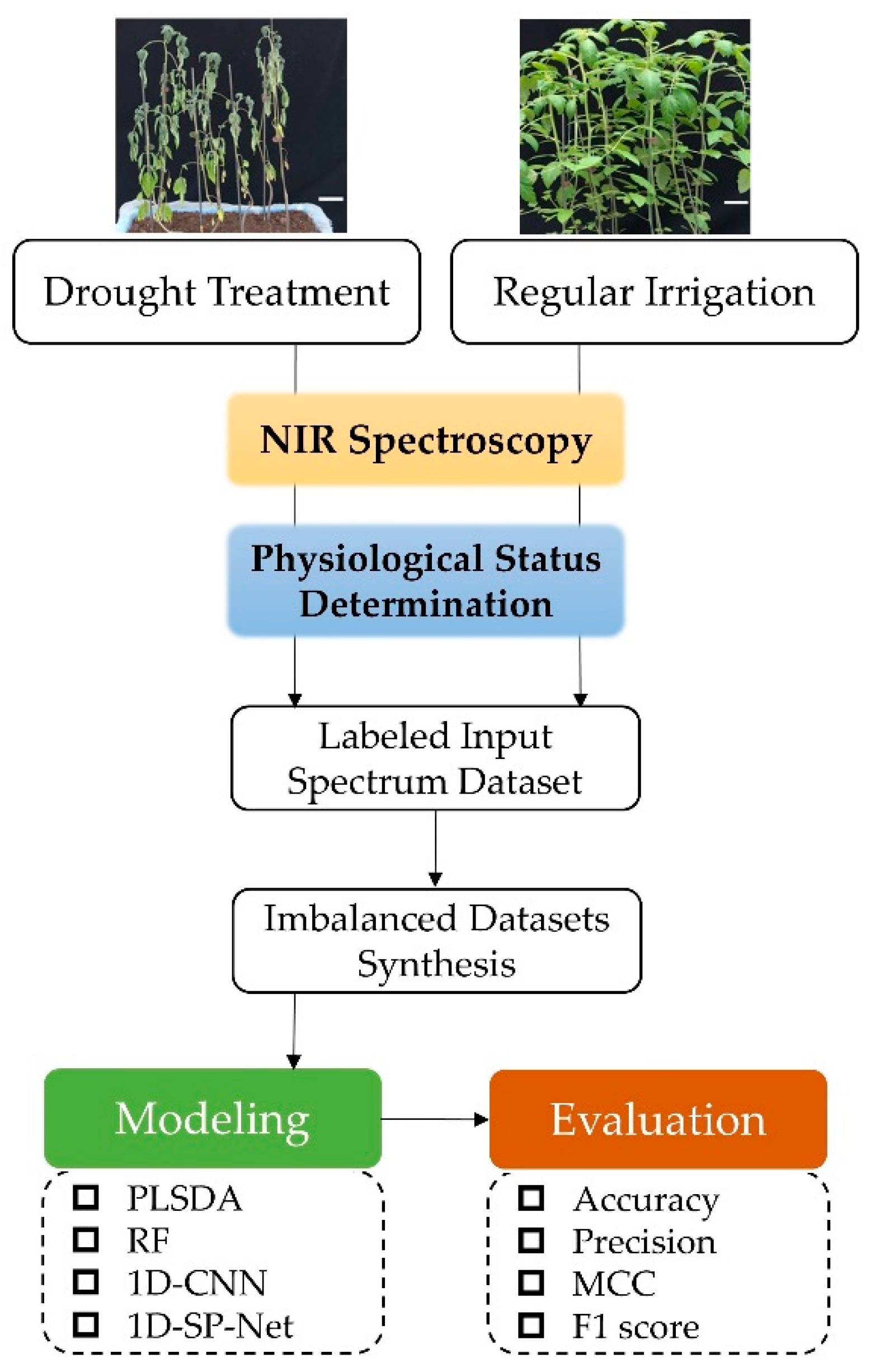
2. Materials and Methods

The workflow of this study is illustrated in Figure 1. Tomato seedlings were cultivated under the condition of drought and regular irrigation treatment, followed by collection of the NIR reflectance spectra. Physiological data were collected the day after treatment (DAT). The spectral data of each measurement were labeled according to corresponding physiological data and used as the input data set to construct the PLSDA, RF, 1D-CNN, and the proposed 1D-SP-Net.

2.1. Experimental Materials and Drought Treatment

The tomato variety “Rosada” was grown in a greenhouse at the Taiwan Agricultural Research Institute (TARI; 24°03′ N, 120°69′ E). Natural sunlight was used as the light source, and the temperature and relative humidity inside the greenhouse were maintained at 26.0–36.0 °C and 75–90%, respectively. Eight young seedlings with 6–8 fully expanded leaves were planted in a pot with 6D soil substrate (BVB, De Lier, Netherlands). For each batch of the experiment, tomato seedlings were irrigated daily to achieve the water levels of regular irrigation and received water until it leaked from the bottom of the pot. For the tomato seedlings receiving the drought treatment, no irrigation was applied from the time they were potted. In total, 12 batches of the experiment were conducted.

2.2. Collection of Physiological Parameters

For each tomato seedling, three fully expanded leaves from below the top of the seedling were examined with the use of a LI-6800 Portable Photosynthesis System (LI-COR Biosciences, Lincoln, NE, USA) to collect data for key physiological status-related parameters. Measurements were taken by clamping the seedlings’ leaves to the quantum sensor of the LI-6800 daily from 09:30 to 12:00. Leaf temperature, assimilation rate (A), transpiration rate (E), stomatal conductance (g_s), and temperature were measured with the LI-6800 at ambient air temperature (27.0–31.0 °C), air humidity (RH = 60%), reference CO₂ concentration (400 μmol/mol⁻¹), and stable light intensity of 1200 μmol photons m⁻² s⁻¹ from an internal light emitting diode light source (red:blue ratio = 9:1). The mean values of A, E, and g_s recorded from three examinations of fully expanded leaves from each individual seedling were counted as one observation. In total, 378 observations of leaf physiological parameters for individual tomato seedlings were collected.

2.3. Physiological Status Determination

The early drought physiological stress status was only confirmed, once the A, E, and g_s parameters of the tomato seedlings in the drought treatment group were all significantly lower than those in the control group (p < 0.05) before the apparent water deficit-related morphological alterations were observed. The physiological status of the seedlings was then marked as “early drought physiological status” and coded as “1”. If one of the parameters A, E, or g_s of the tomato seedlings in the drought treatment group was not significantly lower than those in the control group (p ≥ 0.05) before the apparent water deficit-related morphological alterations were observed, then the status of the seedlings was marked as “normal physiological status” and coded as “0”. Statistically significant differences were determined by performing Student’s t test. In the subsequent analysis, the physiological status of the tomato seedlings was used as the response variable for model construction.

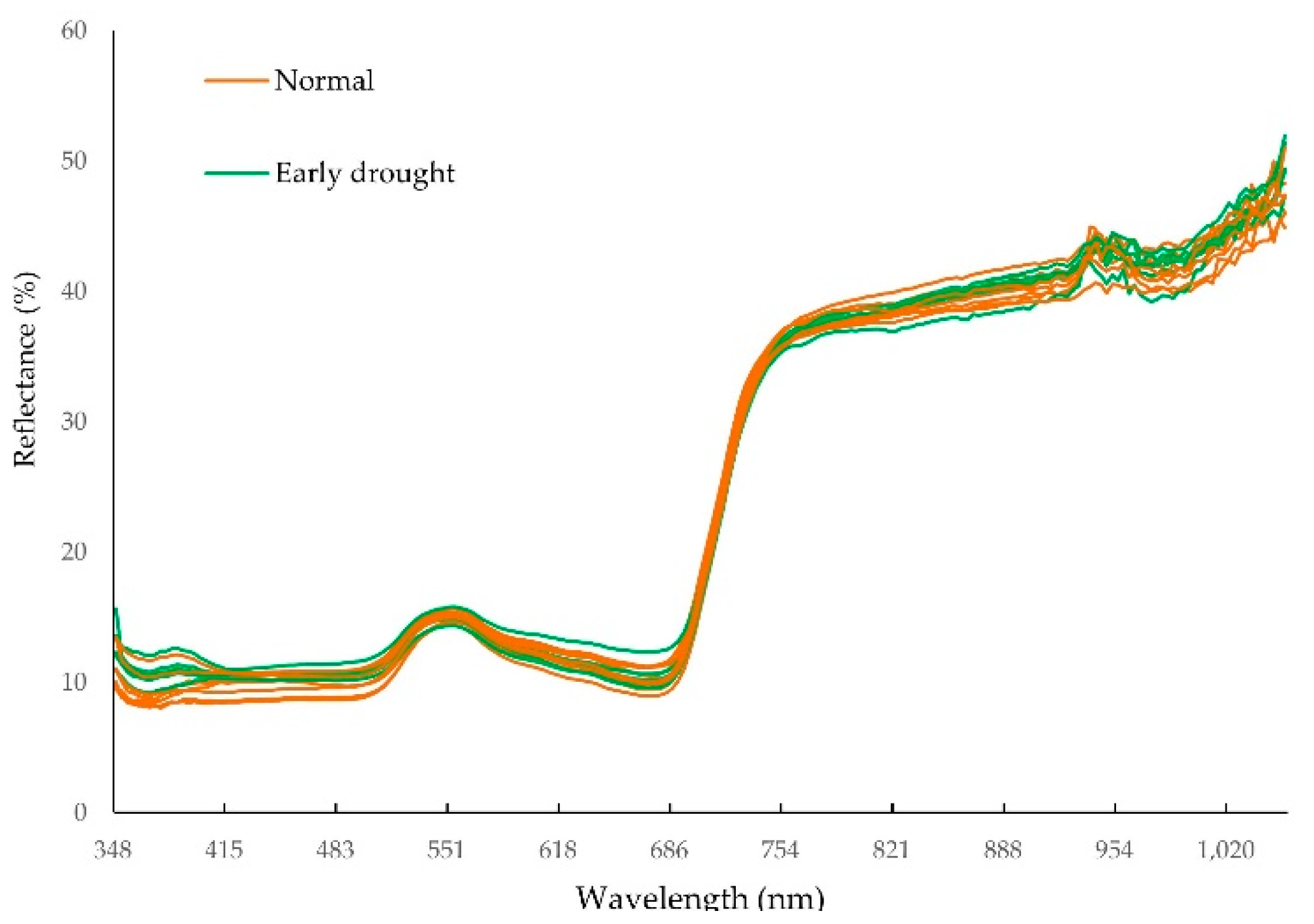
2.4. Collection of NIR Spectral Data

Canopy reflectance within the range of 348–1052 nm was measured at 3-nm intervals by using an MS-720 portable spectroradiometer (EKO Instruments, San Jose, CA, USA). Before the reflectance signal was recorded, the spectroradiometer was calibrated to black and white calibration standard boards and placed at a fixed distance (20 cm) from the tops of the tomato seedlings. From 10:00 to 12:00, the canopy reflectance of each tomato seedling was measured three times; subsequently, the measurements were averaged and any abnormal observations outside the range of 0–1 were excluded. The resulting spectral data were processed by standardization through the following equation:

$${\mathit{x}}_{\mathit{i}\mathit{j}}^{*}=\raisebox{1ex}{$\left({\mathit{x}}_{\mathit{i}\mathit{j}}-{\overline{\mathit{x}}}_{\mathit{i}}\right)$}\!\left/ \!\raisebox{-1ex}{${\mathit{s}}_{\mathit{i}}$}\right.$$

(1)

where ${\mathit{x}}_{\mathit{i}\mathit{j}}^{*}$ is the jth observation value of the ith wavelength after standardization, ${\mathit{x}}_{\mathit{i}\mathit{j}}$ is the jth original observation value of the ith wavelength, ${\overline{\mathit{x}}}_{\mathit{i}}$ is the mean of the ith wavelength, and ${\mathit{s}}_{\mathit{i}}$ is the standard deviation of the ith wavelength.

2.5. Estimation of the Extent of Imbalance and Data Set Synthesis

The extent of the imbalance of the raw data was estimated by using the imbalance ratio (IR). The IR was calculated using the number of the major class (data marked as “normal physiological status”) divided by the number of the minor class (data marked as “early drought physiological status”). Moreover, to evaluate the effects of different degrees of imbalance on the model performance, we simulated synthetic data sets by randomly sampling major and minor classes from the raw data set by using IR = 1 (balance), 10 and 50. The random sampling was performed using dplyr (version 1.0.7) with R (version 4.1.1) statistical software.

2.6. Model Construction

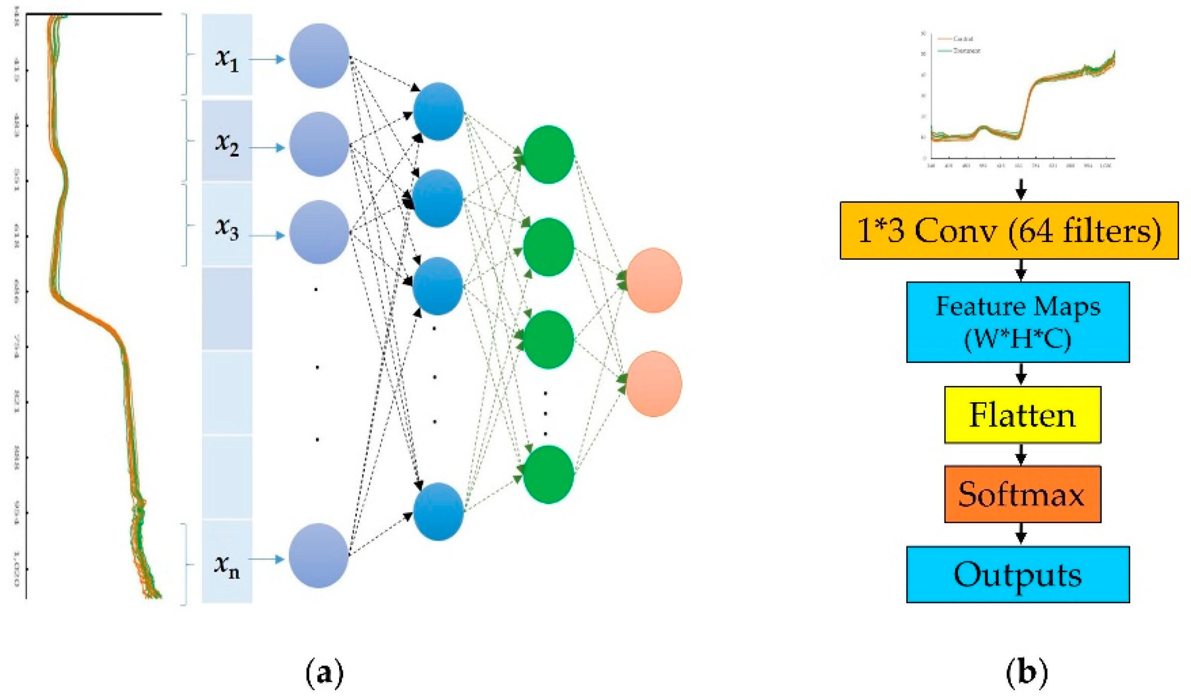
2.6.1. One Dimension Convolutional Neural Network (1D-CNN)

The network architecture of the 1D-CNN model was based on that employed by Acquarelli et al. [45]. As displayed in Figure 2, the 1D-CNN comprised one input layer, one feature map filtered by a 1D kernel and one fully connected layer. The softmax activation function was implemented to map the fully connected layer to a probability distribution for the output layer to conclude the classification results.

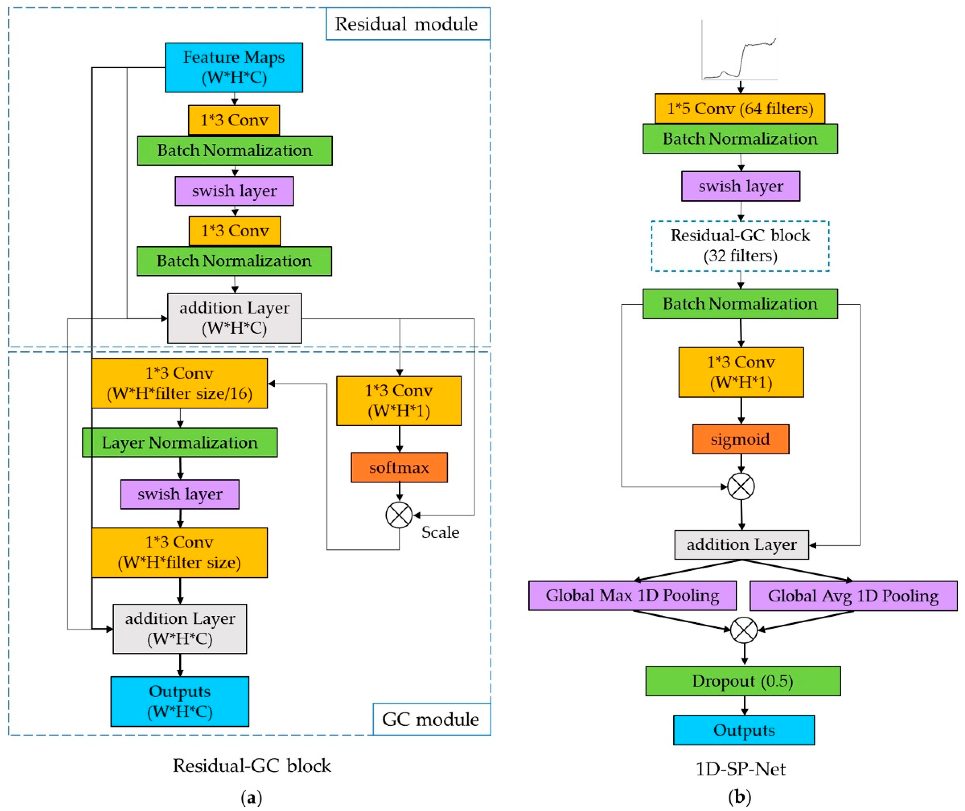
2.6.2. One Dimension Spectrogram Power Net (1D-SP-Net)

We proposed a new architecture for a 1D-CNN model, the 1D-SP-Net, for the sequencing of spectrogram power classification. In addition, a new network block, named residual–GC block, was embedded in the 1D-SP-Net. The overall structure of the residual–GC block and 1D-SP-Net model is displayed in Figure 3. The residual–GC block is composed of two modules: a residual learning module and a GC module. The residual learning and GC modules were constructed with reference to ResNet [56] and global context networks [57], respectively. The residual learning module utilizes skip connections to jump over some layers that could avoid the problem of vanishing gradients and to mitigate the degradation problem. The GC module combines the advantages of both non-local networks [58] and squeeze-and-excitation networks [59] that not only exploits the global context modeling capabilities, but also requires less computation. The filter number of all 1D convolutional layers in the residual–GC block was 32. Except for the softmax and sigmoid activation functions, the swish activation function that was proven to achieve higher test accuracy than ReLU was implemented in the 1D-SP-Net as well [60]. To facilitate training processes and to reduce the gradient vanishing and overfitting, the batch normalization and dropout layers were included in the architecture. The dropout in the 1D-SP-Net was set at 0.5 according to Srivastava et al. [61], which indicated that 0.5 of dropout was close to optimal for an extensive range of networks. In addition to the residual–GC block, a channel-based attention technology that multiplies the global-max 1D-pooling layer by the global-average 1D-pooling layer was used in the 1D-SP-Net. The code of the proposed 1D-SP-Net is publicly available at https://github.com/tariyktu/1D-SP-Net (last accessed date: 9 February 2022).

2.6.3. Partial Least Squares Discriminant Analysis (PLSDA)

PLS is a multivariate method that involves constructing a linear relationship between a set of response variables x and a set of predictor variables y. Let X (dimension I × J) be a matrix of predictive variables of the training data set, and Y the response matrix, with I rows (samples) and G columns (the class information). Each entry $y_{ig}$ of Y represents the membership of the ith sample to the gth class expressed as a binary code (1 or 0). For a given number of dimensions K, the PLS scores denoted T and dimension I × K represent a set of LVs, which are linear combinations of the original variables in X. The coefficients of the linear combinations are gathered in the matrix of loadings P, as shown in Equations (2) and (3).

$$\mathit{T}=\mathit{X}\mathit{P}$$

(2)

As in Equation (3), the regression model associated with K dimensions yields a prediction of Y gathered in the matrix $\widehat{\mathit{Y}}$ and a matrix of estimated regression coefficients B.

$$\widehat{\mathit{Y}}=\mathit{X}\mathit{B}$$

(3)

For the prediction of new observations, PLSDA returns estimated values ($y_{ig}^e$) for each ith sample and for each gth class. To assign a class, the probability that a sample belongs to a specific class can be calculated and the classification of samples is performed by selecting the class that has the highest probability [62]. In this study, the PLSDA algorithm was implemented using the mdatools package (version 0.12.0) in R (version 4.1.1) statistical software.

2.6.4. Random Forest (RF)

The RF model in this study employed the bootstrap strategy to generate several different training data sets with the same proposition of the original data for the purpose of creating many individual CARTs as a tree. Each tree contained nodes that included a certain number of predictive variables (spectral bands). The optimal split and number of the predictive variables in each node was determined according to the minimum Gini index. The RF algorithm was executed using the random forest package (version 4.6–14) in R (version 4.1.1); the parameter ntree, the number of trees to grow, and the parameter mtry, the number of different predictors per node, were set to default values.

2.7. Model Performance Metrics

Common performance metrics, namely accuracy, precision, Matthew’s correlation coefficient (MCC), and F1 scores, which are widely used to evaluate the capability of the models to distinguish between classes, were calculated according to Equations (4)–(7), respectively (

Table 1. Confusion matrix of true conditions and predicted conditions.

		True Condition
		Positive	Negative
Predicted Condition
	Positive	True positive (TP) a	False positive (FP) b
	Negative	False negative (FN) c	True negative (TN) d

^a True physiological status of the tomato seedling is “1” and the model classifies it as “1”; ^b True physiological status of the tomato seedling is “0” but the model classifies it as “1”; ^c True physiological status of the tomato seedling is “1” but the model classifies it as “0”; ^d True physiological status of the tomato seedling is “0” and the model classifies it as “0”.

). These metrics were computed using R (version 4.1.1) or Python (version 3.5.6).

$$\mathrm{Accuracy}=\raisebox{1ex}{$\left(\mathit{T}\mathit{P}+\mathit{T}\mathit{N}\right)$}\!\left/ \!\raisebox{-1ex}{$\left(\mathit{T}\mathit{P}+\mathit{T}\mathit{N}+\mathit{F}\mathit{P}+\mathit{F}\mathit{N}\right)$}\right.$$

(4)

$$\mathrm{Precision}=\raisebox{1ex}{$\mathit{T}\mathit{P}$}\!\left/ \!\raisebox{-1ex}{$\left(\mathit{T}\mathit{P}+\mathit{F}\mathit{P}\right)$}\right.$$

(5)

$$\mathrm{MCC}=\raisebox{1ex}{$\left(\mathit{T}\mathit{P}\times \mathit{T}\mathit{N}\right)-\left(\mathit{F}\mathit{P}\times \mathit{F}\mathit{N}\right)$}\!\left/ \!\raisebox{-1ex}{$\sqrt{\left(\mathit{T}\mathit{N}+\mathit{F}\mathit{N}\right)\left(\mathit{T}\mathit{N}+\mathit{F}\mathit{P}\right)\left(\mathit{T}\mathit{P}+\mathit{F}\mathit{N}\right)\left(\mathit{T}\mathit{P}+\mathit{F}\mathit{P}\right)}$}\right.$$

(6)

$$\mathrm{F}1 \mathrm{score}=\raisebox{1ex}{$2\mathit{T}\mathit{P}$}\!\left/ \!\raisebox{-1ex}{$\left(2\mathit{T}\mathit{P}+\mathit{F}\mathit{P}+\mathit{F}\mathit{N}\right)$}\right.$$

(7)

The NIR spectral data were randomly shuffled and split into 80% and 20% of each class of the original data set or synthetic data set as training and testing data sets, respectively. To tune the training model parameters, 10-fold cross-validation was conducted to optimize the training models. The optimized training models were further evaluated using the testing data set and the listed metrics.

3. Results and Discussion

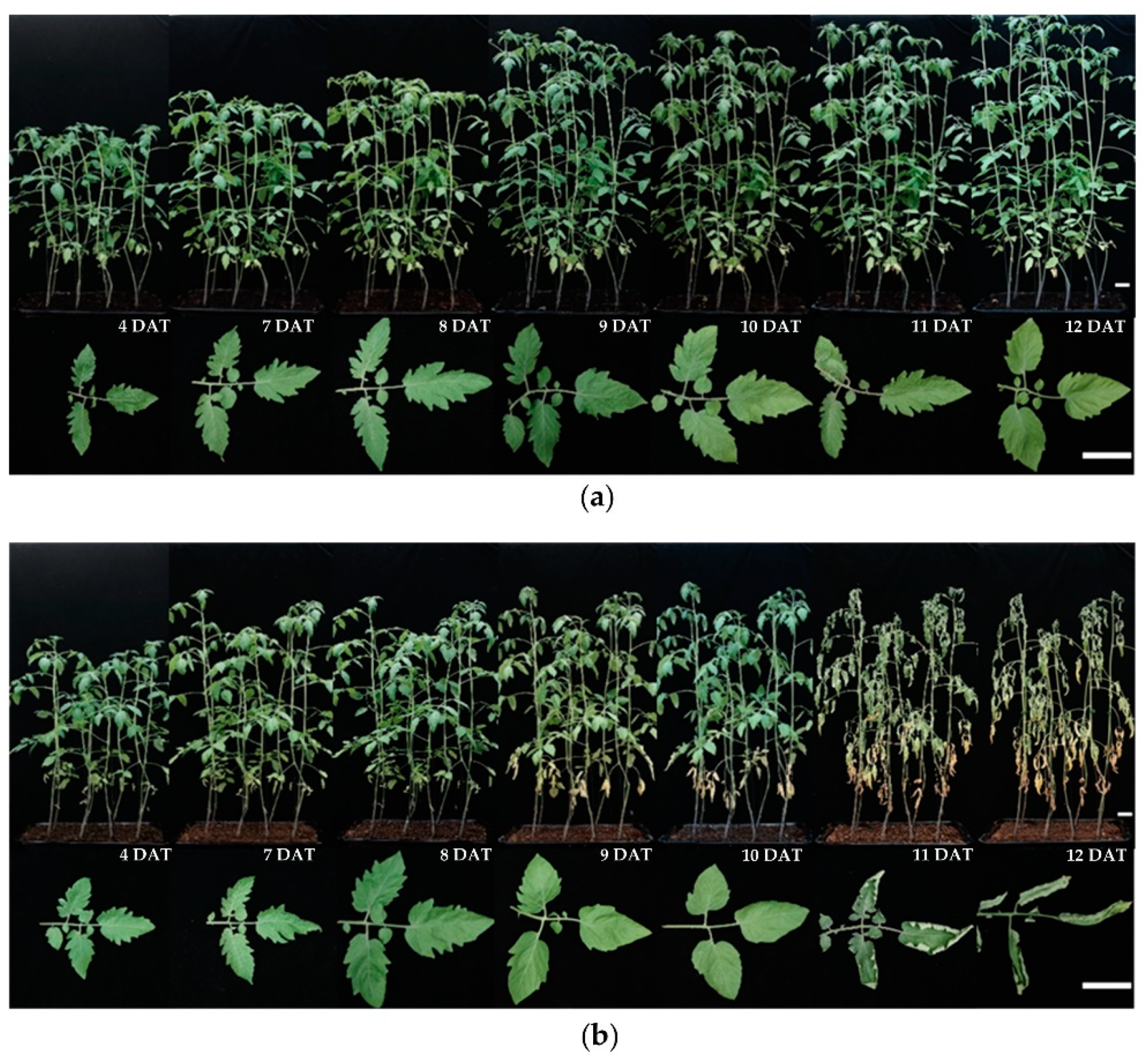
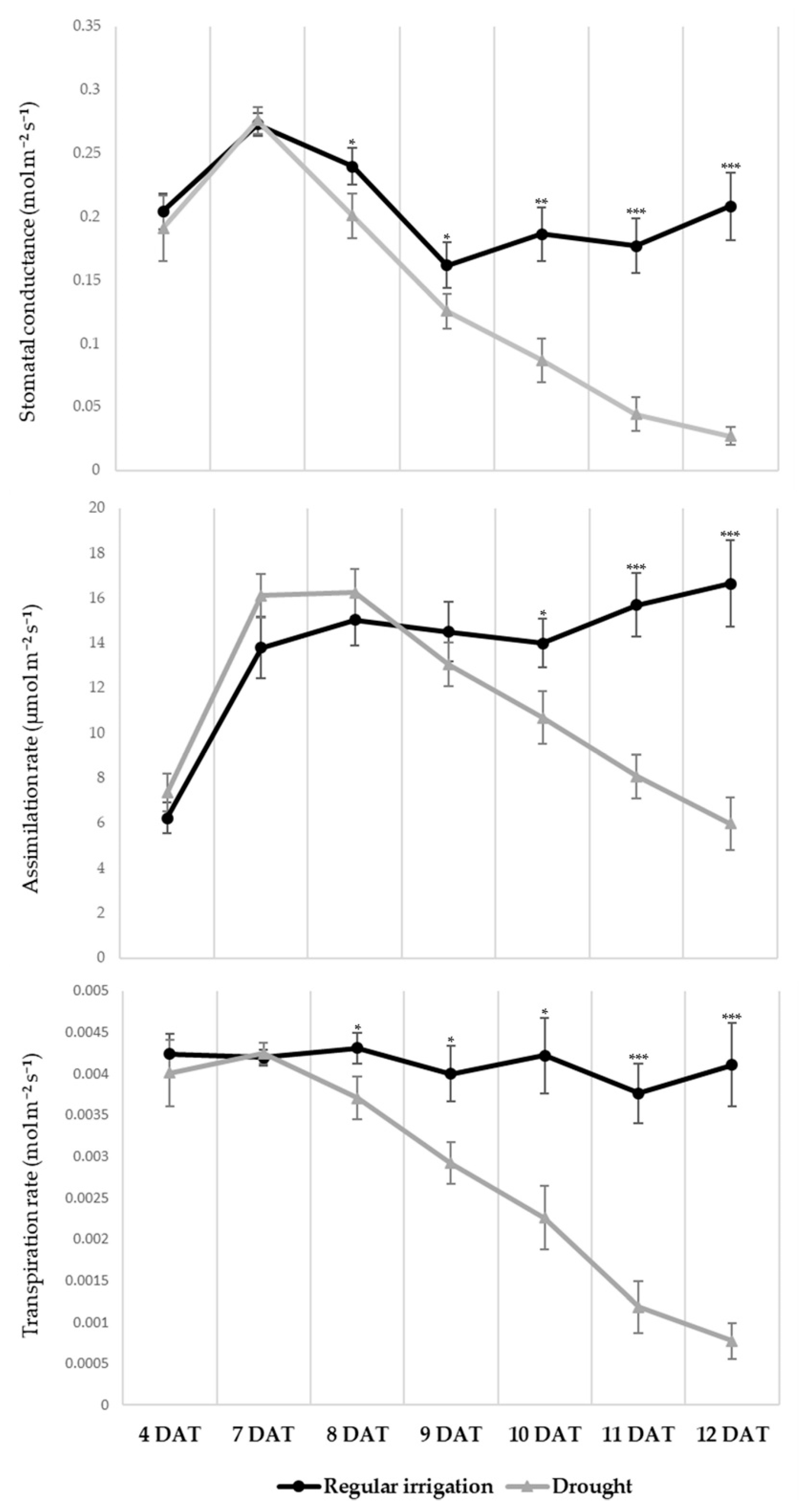
3.1. Morphological and Physiological Alteration under Drought Treatment

The morphological alterations after the regular irrigation and drought treatment are illustrated in Figure 4. Compared with the regular irrigation treatment group, most tomato seedlings in the drought treatment group exhibited apparent water deficit-related morphological alterations, including stalled growth, yellowing and senescence of most leaves on 11 DAT through visual inspection, and continued to develop irreversible damage and eventually wilt. Figure 5 indicates that the g_s and E of the tomato seedlings in the drought treatment group were significantly lower than those in the regular irrigation treatment group at 8 DAT (p < 0.05). From 10 DAT, the A of the tomato seedlings drought group differed significantly from that of the regular irrigation treatment group (p < 0.05). The development of early invisible and late visible morphological alterations in the water-deficit tomato seedlings under the drought conditions was in accordance with the report by Susič et al. [63] that indicated the water deficit led to an initial reduction in g_s and E to prevent the advance of water loss, and lower g_s subsequently constrained the photosynthesis and decreased A. Finally, because of the relocation of nutrients from developed leaves to young leaves to survive under the drought stress, visible leaf senescence occurred [9]. After removing the physiological observations with missing or abnormal value of g_s, E, and A, a total of 378 physiological observations for individual tomato plants were collected. Among the 378 observations, 246 were labeled as “normal physiological status” and 132 observations were labeled as “early physiological drought status”.

Stomata closure is an early response observed under drought conditions, and g_s reduction results in a series of subsequent physiological and biochemical adjustments. The early stages of drought stress are characterized by a notable decline in g_s and E [31,33]. However, the order of alteration in g_s and E under physiological drought status may vary because of individual differences in the genetic backgrounds among individuals of the same species. Furthermore, depending on crop type, divergent definitions of early drought indicators are employed. Mohd Asaari et al. [6] utilized the shrinkage of plant architecture as an indication of the early stages of drought stress for maize (Zea mays). Moreover, in a study of barley (Hordeum vulgare), leaf senescence was a sign for the detection of early drought response [64]. Deviations in responses have even been observed among close relatives; among legume species under drought conditions, stomatal closure was observed for snap beans (Phaseolus vulgaris), whereas cowpeas (Vigna unguiculata) remained partially open [65]. Additionally, some other biotic stresses can induce the indiscriminate physiological alterations resulting from the drought stress. The alterations in the stomatal conductivity, transpiration, and net photosynthesis induced by the nematode (Meloidogyne ethiopica) infection were reported to be similar to the drought stress in tomatoes [66]. Hence, a more stringent definition is necessary to determine the early stages of the drought stress. In this study, the early stages of the physiological drought status were defined as the values of g_s, E, and A simultaneously lower than those of well-watered tomatoes before apparent water deficit–related morphological alterations were visible. Based on the above definition, 246 and 132 observations were labeled as “normal physiological status” and “early physiological drought status”, respectively. The NIR spectra that corresponded to “normal physiological status” and “early physiological drought status” for tomato plants are shown as Figure 6.

3.2. Comparison of Model Performance

The prediction performances of the models were evaluated through several metrics, namely accuracy, precision, MCC, and F1 scores (

Table 2. Comparison of predictive performance for PLSDA, RF, 1D-CNN, and 1D-SP-Net models by accuracy, precision, MCC, and F1 score metrics.

Model	Training				Testing
	Accuracy (%)	Precision (%)	MCC	F1 Score	Accuracy (%)	Precision (%)	MCC	F1 Score
PLSDA	93.2	90.4	0.85	0.90	86.7	82.9	0.70	0.80
RF	81.1	75.6	0.58	0.71	77.2	68.4	0.49	0.67
1D-CNN	90.0	88.0	0.79	0.87	90.0	80.0	0.74	0.80
1D-SP-Net	96.0 a	93.1	0.91	0.94	96.3	98.0	0.92	0.95

^a Bold characters represent the highest values for a respective metric among the models.

). Overall, the 1D-SP-Net outperformed the PLSDA, RF, and 1D-CNN models according to the training and testing results. The PLSDA and 1D-CNN models exhibited mutually comparable performance, and the RF model recorded the lowest values for accuracy, precision, MCC, and F1 score, both in the results for training and for testing. Furthermore, the accuracy, precision, MCC, and F1 scores of the PLSDA, RF, and 1D-CNN models were lower in the testing results than in the training results (Figure 7). By contrast, the 1D-SP-Net exhibited relatively stable and even slightly increased values for all the evaluation metrics in the testing results compared with those of the training results.

In this study, the most favorable model performance was observed in the proposed 1D-SP-Net model which reached accuracy of 96.3%, precision of 98.0%, MCC of 0.92, and F1 score of 0.95. (Table 2). Residual learning was able to mitigate the training error and the computational complexity as the depth of the neural network increased [56], and the GC module, which employs self-attention learning, enabled the model to discern the key relationships between global and local features [57]. The residual and GC modules were embedded in the proposed 1D-SP-Net, thus contributing to the prediction performance. Our results are consistent with those of Zhao et al. [67], who reported improvements in a CNN model after the embedding of residual blocks and GC modules; that model subsequently achieved an average accuracy above 96% in identifying tomato leaf diseases. Furthermore, compared to training results, the PLSDA, RF, and 1D-CNN models revealed non-negligible reductions ranging from 4.8% to 17.6% to the accuracy, precision, MCC, and F1 scores in testing results (Figure 7). The lower model performance observed in the testing results indicated the occurrence of overfitting. By contrast, the proposed 1D-SP-Net exhibited relatively consistent accuracy (0.3% increment), MCC (1.1%) increment F1 scores (1.1% increment), and slightly increased precision (5.4% increment) in the testing results, indicating that the proposed 1D-SP-Net is more robust to overfitting than the other models (Figure 7).

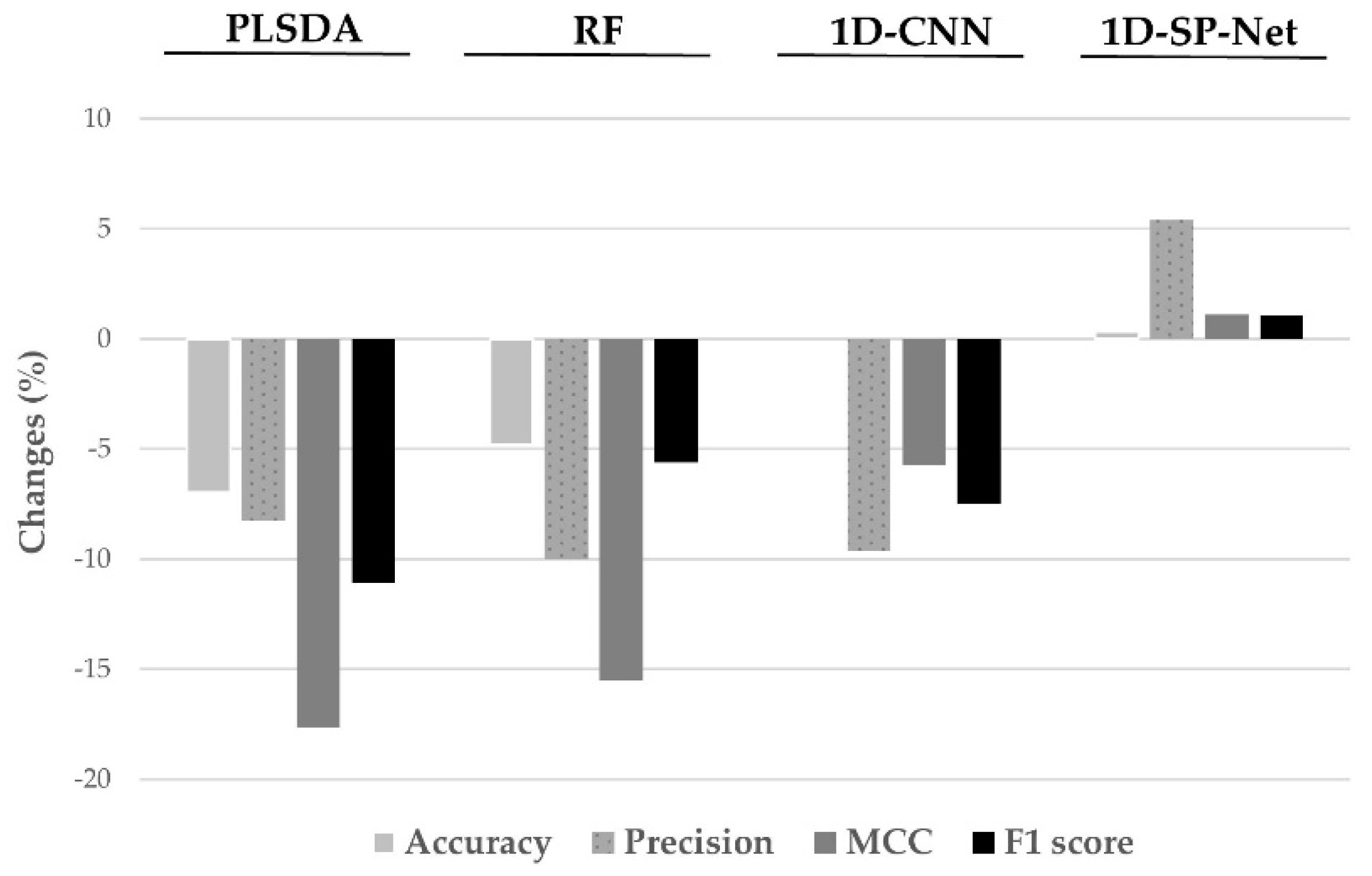
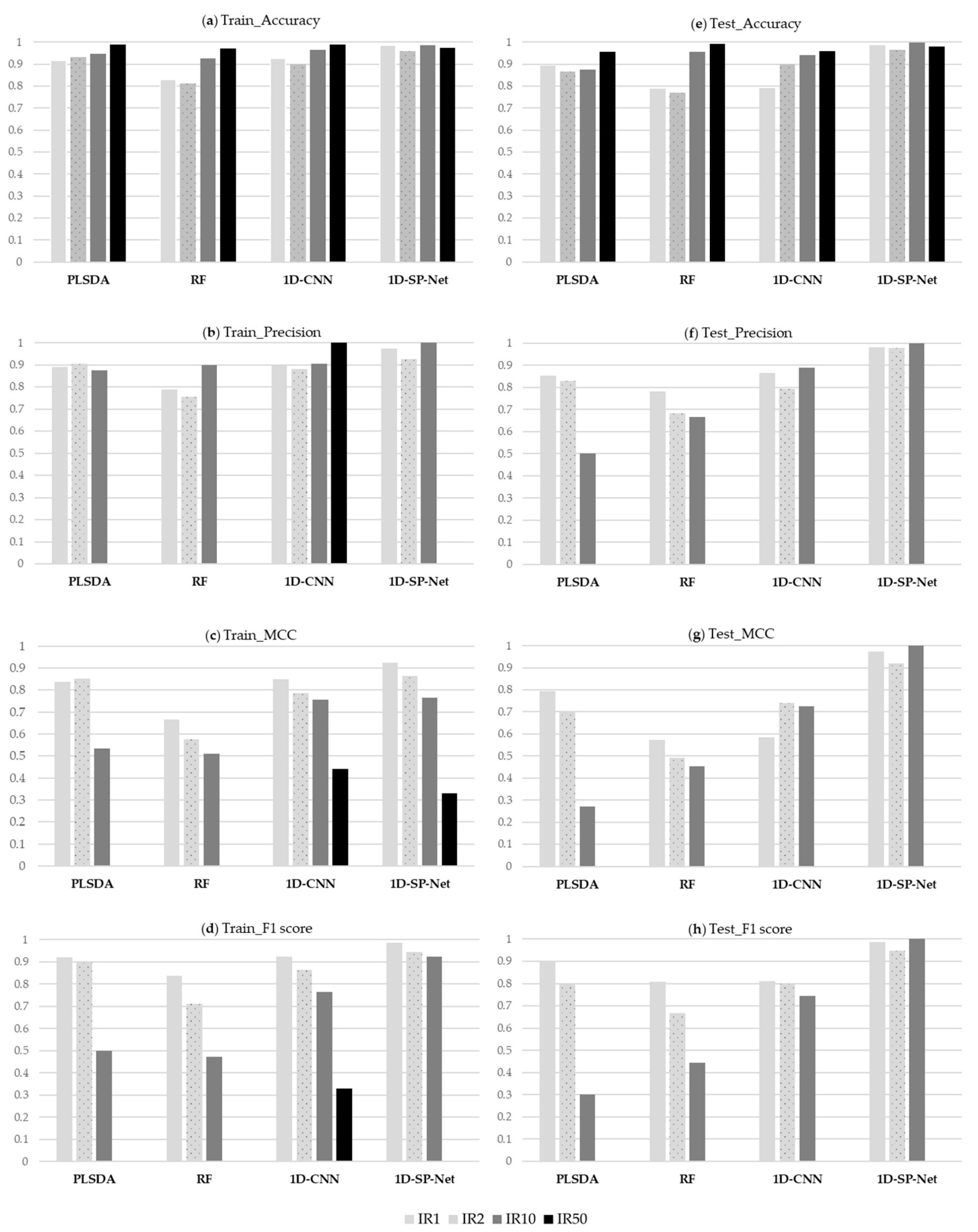
3.3. Effects of the Extent of Imbalance on Model Performance

The IR of the data set in this study was approximately 2, which represented slight imbalance (

Table 3. Extent of the imbalance in the data sets used in this study.

Dataset	Type	Imbalance Ratio	Major Class b	Minor Class c
IR1	Synthetic a	1	189	189
IR2	Original dataset	2	246	132
IR10	Synthetic	10	340	38
IR50	Synthetic	50	370	8

^a Synthetic data set was established by random sampling from the original data set; ^b Number of observations that was classed as “normal physiological status”; ^c Number of observations that was classed as “early physiological drought status”.

). Therefore, with the aim of evaluating the influence of imbalance on the models, we fixed the sample size and simulated a balanced data set with IR equal to one. Additionally, we subjected the models to more severely imbalanced data sets with IRs equal to 10 and 50 through random sampling from the original data set (IR2).

For a classification problem, using suitable metrics that can reflect the real distinguishing capacity of the model is essential. The accuracy paradox indicates that the use of the metric accuracy is impractical because of its poor perception of the imbalance of class distribution [68]. Instead, the MCC has been reported to be a suitable metric for measuring classification performance, especially for models constructed through the use of imbalanced data sets [69]. The metric F1 score has been widely used for binary and multiclass scenarios and is less influenced by factors related to class imbalance [70]. In the present study, to comprehensively evaluate the prediction performance of the PLSDA, RF, 1D-CNN, and 1D-SP-Net models when fitting data sets with various degrees of imbalance, metrics commonly used in machine learning, namely precision, accuracy, MCC, and F1 scores were used to measure model performance (Figure 8).

Figure 8 reveals the training and testing results for all the models using different IR data sets. The proposed 1D-SP-Net exhibited the most consistent and the highest accuracy, precision, MCC, and F1 scores. Notably, accuracy remained relatively unaffected or even increased slightly in the training and testing results as the extent of the imbalance became greater, indicating that the accuracy metric was unable to reflect the effects of class imbalance and represented overoptimistic evaluation results. The values for precision exhibited a similar tendency as those for accuracy in the training results but revealed small decreases as the extent of imbalance got higher in the testing results. The metrics of accuracy and precision were not suitable for evaluating models with class-imbalance problems. The training and testing results for the MCC and F1 scores revealed that the prediction performances for PLSDA and RF had a decreasing tendency as the extent of the imbalance increased. The larger the extent of the imbalance of the data set was, the more substantial was its influence on model performance. Regarding the CNN-based model, as the extent of imbalance in the data set increased, the 1D-CNN displayed comparable MCC and higher F1 scores compared with those of the PLSDA and RF models. The proposed 1D-SP-Net not only revealed more favorable MCC and F1 scores than those of the 1D-CNN but also exhibited consistently higher MCC and F1 scores both in training and testing results. These results indicated that the proposed 1D-SP-Net outperformed other models in overall prediction performance and robustness.

4. Conclusions

The establishment of a reliable and nondestructive method for determining the occurrence of stress in its early stages is of great significance for agricultural research and for the development of agricultural applications. In the context of machine learning, most research has successfully addressed the class-imbalance problem by employing CNN architecture, yet studies have seldom applied CNNs to the field of agricultural research. In this study, we proposed the 1D-SP-Net embedded with residual blocks and GC blocks to predict the early physiological drought status of tomato seedlings. In the testing results, the 1D-SP-Net exhibited an accuracy of 96.3%, precision of 98.0%, an MCC of 0.92, and an F1 score of 0.95. All these performance values of the 1D-SP-Net exceeded those of the PLSDA, RF, and 1D-CNN models. Furthermore, when fitting data sets with varying degrees of imbalance, the proposed 1D-SP-Net revealed the highest values for MCC and F1 scores, both in training and in testing results. Our results indicated that the 1D-SP-Net is a promising model that can determine the early drought stress status of tomato seedlings in a noninvasive manner and is more robust and resistant to the effects of imbalanced data sets than PLSDA, RF, and 1D-CNN models.

References

1. Taiz, L.; Zeiger, E.; Møller, I.M.; Murphy, A. Plant Physiology and Development, 6th ed.; Sinauer Associates Incorporated: Sunderland, MA, USA, 2015; p. 761. [Google Scholar]
2. Zhao, Y.; Jiang, B.; Huo, Y.; Yi, H.; Tian, H.; Wu, H.; Wang, R.; Zhao, J.; Wang, F. A high-performance database management system for managing and analyzing large-scale SNP data in plant genotyping and breeding applications. Agriculture 2021, 11, 1027. [Google Scholar] [CrossRef]
3. Marsh, J.I.; Hu, H.; Gill, M.; Batley, J.; Edwards, D. Crop breeding for a changing climate: Integrating phenomics and genomics with bioinformatics. Theor. Appl. Genet. 2021, 134, 1677–1690. [Google Scholar] [CrossRef] [PubMed]
4. Singh, P.; Pandey, P.C.; Petropoulos, G.P.; Pavlides, A.; Srivastava, P.K.; Koutsias, N.; Deng, K.A.K.; Bao, Y. Hyperspectral remote sensing in precision agriculture: Present status, challenges, and future trends. In Hyperspectral Remote Sensing; Elsevier: Amsterdam, The Netherlands, 2020; pp. 121–146. [Google Scholar]
5. Liaghat, S.; Ehsani, R.; Mansor, S.; Shafri, H.Z.M.; Meon, S.; Sankaran, S.; Azam, S.H.M.N. Early detection of basal stem rot disease (Ganoderma) in oil palms based on hyperspectral reflectance data using pattern recognition algorithms. Int. J. Remote Sens. 2014, 35, 3427–3439. [Google Scholar] [CrossRef]
6. Mohd Asaari, M.S.; Mishra, P.; Mertens, S.; Dhondt, S.; Inzé, D.; Wuyts, N.; Scheunders, P. Close-range hyperspectral image analysis for the early detection of stress responses in individual plants in a high-throughput phenotyping platform. ISPRS J. Photogramm. Remote Sens. 2018, 138, 121–138. [Google Scholar] [CrossRef]
7. Jamalluddin, N.; Massawe, F.J.; Mayes, S.; Ho, W.K.; Singh, A.; Symonds, R.C. Physiological screening for drought tolerance traits in vegetable amaranth (Amaranthus tricolor) germplasm. Agriculture 2021, 11, 994. [Google Scholar] [CrossRef]
8. Alseekh, S.; Bermudez, L.; de Haro, L.A.; Fernie, A.R.; Carrari, F. Crop metabolomics: From diagnostics to assisted breeding. Metab. Off. J. Metab. Soc. 2018, 14. [Google Scholar] [CrossRef] [Green Version]
9. Distelfeld, A.; Avni, R.; Fischer, A.M. Senescence, nutrient remobilization, and yield in wheat and barley. J. Exp. Bot. 2014, 65, 3783–3798. [Google Scholar] [CrossRef] [Green Version]
10. Feng, Y.X.; Chen, X.; Li, Y.W.; Zhao, H.M.; Xiang, L.; Li, H.; Cai, Q.Y.; Feng, N.X.; Mo, C.H.; Wong, M.H. A visual leaf zymography technique for the in situ examination of plant enzyme activity under the stress of environmental pollution. J. Agric. Food Chem. 2020, 68, 14015–14024. [Google Scholar] [CrossRef]
11. Janni, M.; Gulli, M.; Maestri, E.; Marmiroli, M.; Valliyodan, B.; Nguyen, H.T.; Marmiroli, N. Molecular and genetic bases of heat stress responses in crop plants and breeding for increased resilience and productivity. J. Exp. Bot. 2020, 71, 3780–3802. [Google Scholar] [CrossRef]
12. Huang, L.; Wu, K.; Huang, W.; Dong, Y.; Ma, H.; Liu, Y.; Liu, L. Detection of fusarium head blight in wheat ears using continuous wavelet analysis and PSO-SVM. Agriculture 2021, 11, 998. [Google Scholar] [CrossRef]
13. Ribera-Fonseca, A.; Jorquera-Fontena, E.; Castro, M.; Acevedo, P.; Parra, J.C.; Reyes-Diaz, M. Exploring VIS/NIR reflectance indices for the estimation of water status in high bush blueberry plants grown under full and deficit irrigation. Sci. Hortic. 2019, 256, 108557. [Google Scholar] [CrossRef]
14. Diago, M.P.; Fernández-Novales, J.; Gutiérrez, S.; Marañón, M.; Tardaguila, J. Development and validation of a new methodology to assess the vineyard water status by on-the-go near infrared spectroscopy. Front. Plant Sci. 2018, 9, 59. [Google Scholar] [CrossRef] [PubMed] [Green Version]
15. Steidle Neto, A.J.; de O Moura, L.; de C. Lopes, D.; de A Carlos, L.; Martins, L.M.; de C Louback Ferraz, L. Non-destructive prediction of pigment content in lettuce based on visible-NIR spectroscopy. J. Sci. Food Agric. 2017, 97, 2015–2022. [Google Scholar] [CrossRef] [PubMed]
16. Jensen, J.R. Remote Sensing of the Environment: An Earth Resource Perspective 2/e; Pearson Prentice Hall: Upper Saddle River, NJ, USA, 2007. [Google Scholar]
17. Nie, P.; Xia, Z.; Sun, D.W.; He, Y. Application of visible and near infrared spectroscopy for rapid analysis of chrysin and galangin in Chinese propolis. Sensors 2013, 13, 10539–10549. [Google Scholar] [CrossRef] [PubMed] [Green Version]
18. Barker, M.J.; Hussan, S.R.; Lovergne, L.; Untereiner, V.; Hughes, C.; Lukaszewski, R.A.; Thiéfinbg, G.; Sockalingum, G.D. Developing and understanding biofluid vibrational spectroscopy: A critical review. Chem. Soc. Rev. 2016, 45, 1803–1818. [Google Scholar] [CrossRef] [Green Version]
19. Pandiselvam, R.; Mahanti, N.K.; Manikantan, M.R.; Kothakota, A.; Chakraborty, S.K.; Ramesh, S.V.; Beegum, P.S. Rapid detection of adulteration in desiccated coconut powder: Vis-NIR spectroscopy and chemometric approach. Food Control 2022, 133, 108588. [Google Scholar] [CrossRef]
20. Das, B.; Manohara, K.K.; Mahajan, G.R.; Sahoo, R.N. Spectroscopy based novel spectral indices, PCA- and PLSR-coupled machine learning models for salinity stress phenotyping of rice. Spectrochim. Acta A Mol. Biomol. Spectrosc. 2020, 229, 117983. [Google Scholar] [CrossRef]
21. Marín-Ortiz, J.C.; Gutierrez-Toro, N.; Botero-Fernández, V.; Hoyos-Carvajal, L.M. Linking physiological parameters with visible/near-infrared leaf reflectance in the incubation period of vascular wilt disease. Saudi J. Biol. Sci. 2020, 27, 8899. [Google Scholar] [CrossRef]
22. Genc, L.; Inalpulat, M.; Kizil, U.; Mirik, M.; Smith, S.E.; Mendes, M. Determination of water stress with spectral reflectance on sweet corn (Zea mays L.) using classification tree (CT) analysis. Zemdirb. Agric. 2013, 100, 81–90. [Google Scholar] [CrossRef]
23. Tu, Y.-K.; Chen, H.-W.; Fang, S.-L.; Yao, M.-H.; Tseng, Y.-Y.; Kuo, B.-J. Establishing of early discrimination methods for drought stress of tomato by using environmental parameters and NIR spectroscopy in greenhouse. Acta Hortic. 2021, 1311, 501–512. [Google Scholar] [CrossRef]
24. Osco, L.P.; Ramos, A.P.M.; Moriya, É.A.S.; Bavaresco, L.G.; de Lima, B.C.; Estrabis, N.; Pereira, D.R.; Creste, J.E.; Júnior, J.M.; Gonçalves, W.N.; et al. Modeling hyperspectral response of water-stress induced lettuce plants using artificial neural networks. Remote Sens. 2019, 11, 2797. [Google Scholar] [CrossRef] [Green Version]
25. Maimaitiyiming, M.; Ghulam, A.; Bozzolo, A.; Wilkins, J.L.; Kwasniewski, M.T. Early detection of plant physiological responses to different levels of water stress using reflectance spectroscopy. Remote Sens. 2017, 9, 745. [Google Scholar] [CrossRef] [Green Version]
26. Ihuoma, S.O.; Madramootoo, C.A. Sensitivity of spectral vegetation indices for monitoring water stress in tomato plants. Comput. Electron. Agric. 2019, 163. [Google Scholar] [CrossRef]
27. Romero, A.P.; Alarcón, A.; Valbuena, R.I.; Galeano, C.H. Physiological assessment of water stress in potato using spectral information. Front. Plant Sci. 2017, 8, 1608. [Google Scholar] [CrossRef] [PubMed]
28. Sanseechan, P.; Panduangnate, L.; Saengprachatanarug, K.; Wongpichet, S.; Taira, E.; Posom, J. A portable near infrared spectrometer as a non-destructive tool for rapid screening of solid density stalk in a sugarcane breeding program. Sens. Bio-Sens. Res. 2018, 20, 34–40. [Google Scholar] [CrossRef]
29. Gutiérrez, S.; Tardaguila, J.; Fernández-Novales, J.; Diago, M.P. Data mining and NIR spectroscopy in viticulture: Applications for plant phenotyping under field conditions. Sensors 2016, 16, 236. [Google Scholar] [CrossRef] [Green Version]
30. Vilmus, I.; Ecarnot, M.; Verzelen, N.; Roumet, P. Monitoring nitrogen leaf resorption kinetics by near-infrared spectroscopy during grain filling in durum wheat in different nitrogen availability conditions. Crop Sci. 2014, 54, 284–296. [Google Scholar] [CrossRef]
31. Omena-Garcia, R.P.; Oliveira Martins, A.; Medeiros, D.B.; Vallarino, J.G.; Mendes Ribeiro, D.; Fernie, A.R.; Araújo, W.L.; Nunes-Nesi, A. Growth and metabolic adjustments in response to gibberellin deficiency in drought stressed tomato plants. Environ. Exp. Bot. 2019, 159, 95–107. [Google Scholar] [CrossRef]
32. Giordano, M.; Petropoulos, S.A.; Rouphael, Y. Response and defence mechanisms of vegetable crops against drought, heat and salinity stress. Agriculture 2021, 11, 463. [Google Scholar] [CrossRef]
33. Liang, G.; Liu, J.; Zhang, J.; Guo, J. Effects of drought stress on photosynthetic and physiological parameters of tomato. J. Am. Soc. Hortic. Sci. 2020, 145, 12–17. [Google Scholar] [CrossRef] [Green Version]
34. Dardenne, P.; Sinnaeve, G.; Baeten, V. Multivariate calibration and chemometrics for near infrared spectroscopy: Which method? J. Near Infrared Spectrosc. 2000, 8, 229–237. [Google Scholar] [CrossRef]
35. Boulesteix, A.L.; Strimmer, K. Partial least squares: A versatile tool for the analysis of high-dimensional genomic data. Brief. Bioinform. 2006, 8, 32–44. [Google Scholar] [CrossRef] [PubMed] [Green Version]
36. Deng, B.C.; Yun, Y.H.; Liang, Y.Z.; Cao, D.S.; Xu, Q.S.; Yi, L.Z.; Huang, X. A new strategy to prevent over-fitting in partial least squares models based on model population analysis. Anal. Chim. Acta 2015, 880, 32–41. [Google Scholar] [CrossRef] [PubMed]
37. Gowen, A.A.; Downey, G.; Esquerre, C.; O’Donnell, C.P. Preventing over-fitting in PLS calibration models of near-infrared (NIR) spectroscopy data using regression coefficients. J. Chemom. 2011, 25, 375–381. [Google Scholar] [CrossRef]
38. Chen, Y.Y.; Wang, Z.B. Quantitative analysis modeling of infrared spectroscopy based on ensemble convolutional neural networks. Chemometr. Intell. Lab. Syst. 2018, 181, 1–10. [Google Scholar] [CrossRef]
39. De Santana, F.B.; de Souza, A.M.; Poppi, R.J. Visible and near infrared spectroscopy coupled to random forest to quantify some soil quality parameters. Spectrochim. Acta A Mol. Biomol. Spectrosc. 2018, 191, 454–462. [Google Scholar] [CrossRef] [PubMed]
40. Genuer, R.; Poggi, J.M.; Tuleau-Malot, C.; Villa-Vialaneix, N. Random forests for big data. Big Data Res. 2017, 9, 28–46. [Google Scholar] [CrossRef]
41. Lecun, Y.; Bottou, L.; Bengio, Y.; Haffner, P. Gradient-based learning applied to document recognition. Proc. IEEE Inst. Electr. Electron. Eng. 1998, 86, 2278–2324. [Google Scholar] [CrossRef] [Green Version]
42. Giménez, M.; Palanca, J.; Botti, V. Semantic-based padding in convolutional neural networks for improving the performance in natural language processing. A case of study in sentiment analysis. Neurocomputing 2020, 378, 315–323. [Google Scholar] [CrossRef]
43. Kruthika, K.R.; Rajeswari; Maheshappa, H.D. CBIR system using Capsule Networks and 3D CNN for Alzheimer’s disease diagnosis. Inform. Med. Unlocked 2019, 14, 59–68. [Google Scholar] [CrossRef]
44. Kuo, C.-E.; Chen, G.-T.; Liao, P.-Y. An EEG spectrogram-based automatic sleep stage scoring method via data augmentation, ensemble convolution neural network, and expert knowledge. Biomed. Signal Process. Control 2021, 70, 102981. [Google Scholar] [CrossRef]
45. Acquarelli, J.; van Laarhoven, T.; Gerretzen, J.; Tran, T.N.; Buydens, L.M.C.; Marchiori, E. Convolutional neural networks for vibrational spectroscopic data analysis. Anal. Chim. Acta 2017, 954, 22–31. [Google Scholar] [CrossRef] [PubMed] [Green Version]
46. Malek, S.; Melgani, F.; Bazi, Y. One-dimensional convolutional neural networks for spectroscopic signal regression. J. Chemom. 2018, 32, e2977. [Google Scholar] [CrossRef]
47. Zhu, R.; Guo, Y.; Xue, J.H. Adjusting the imbalance ratio by the dimensionality of imbalanced data. Pattern Recognit. Lett. 2020, 133, 217–223. [Google Scholar] [CrossRef]
48. Lee, W.; Jun, C.H.; Lee, J.S. Instance categorization by support vector machines to adjust weights in AdaBoost for imbalanced data classification. Inf. Sci. 2017, 381, 92–103. [Google Scholar] [CrossRef]
49. Somasundaram, A.; Reddy, U.S. Modelling a stable classifier for handling large scale data with noise and imbalance. In Proceedings of the 2017 International Conference on Computational Intelligence in Data Science, Chennai, India, 2–3 June 2017. [Google Scholar] [CrossRef]
50. Nemoto, K.; Hamaguchi, R.; Imaizumi, T.; Hikosaka, S. Classification of rare building change using CNN with multi-class focal loss. In Proceedings of the 2018 IEEE International Geoscience and Remote Sensing Symposium, Valencia, Spain, 22–27 July 2018. [Google Scholar] [CrossRef]
51. Buda, M.; Maki, A.; Mazurowski, M.A. A systematic study of the class imbalance problem in convolutional neural networks. Neural Netw. 2018, 106, 249–259. [Google Scholar] [CrossRef] [Green Version]
52. Ding, W.; Huang, D.Y.; Chen, Z.; Yu, X.; Lin, W. Facial action recognition using very deep networks for highly imbalanced class distribution. In Proceedings of the 2017 Asia-Pacific Signal and Information Processing Association Annual Summit and Conference, Kuala Lumpur, Malaysia, 12–15 December 2017. [Google Scholar] [CrossRef]
53. Khan, S.H.; Hayat, M.; Bennamoun, M.; Sohel, F.A.; Togneri, R. Cost-sensitive learning of deep feature representations from imbalanced data. IEEE Trans. Neural Netw. Learn. Syst. 2018, 29, 3573–3587. [Google Scholar] [CrossRef] [Green Version]
54. He, K.; Sun, J. Convolutional neural networks at constrained time cost. In Proceedings of the 2015 IEEE Conference on Computer Vision and Pattern Recognition, Boston, MA, USA, 7–12 June 2015. [Google Scholar] [CrossRef] [Green Version]
55. Glorot, X.; Bengio, Y. Understanding the difficulty of training deep feedforward neural networks. J. Mach. Learn. Res. 2010, 9, 249–256. [Google Scholar]
56. He, K.; Zhang, X.; Ren, S.; Sun, J. Deep residual learning for image recognition. In Proceedings of the 2016 IEEE Conference on Computer Vision and Pattern Recognition, Las Vegas, NV, USA, 27–30 June 2016. [Google Scholar] [CrossRef] [Green Version]
57. Cao, Y.; Xu, J.; Lin, S.; Wei, F.; Hu, H. Gcnet: Non-local networks meet squeeze-excitation networks and beyond. In Proceedings of the IEEE/CVF International Conference on Computer Vision Workshops, Seoul, Korea, 27–28 October 2019. [Google Scholar] [CrossRef] [Green Version]
58. Wang, X.; Girshick, R.; Gupta, A.; He, K. Non-local neural networks. arXiv 2018, arXiv:1711.07971v3. [Google Scholar]
59. Hu, J.; Shen, L.; Sun, G. Squeeze-and-excitation networks. arXiv 2017, arXiv:1709.01507. [Google Scholar]
60. Ramachandran, P.; Zoph, B.; Le, Q.V. Searching for activation functions. arXiv 2017, arXiv:1710.05941. [Google Scholar]
61. Srivastava, N.; Hinton, G.; Krizhevsk, A.; Sutskever, I.; Salakhutdinov, R. Dropout: A simple way to prevent neural networks from overfitting. J. Mach. Learn. Res. 2014, 15, 1929–1958. [Google Scholar]
62. Chevallier, S.; Bertrand, D.; Kohler, A.; Courcoux, P. Application of PLS-DA in multivariate image analysis. J. Chemom. 2006, 20, 221–229. [Google Scholar] [CrossRef]
63. Susič, N.; Žibrat, U.; Širca, S.; Strajnar, P.; Razinger, J.; Knapič, M.; Vončina, A.; Urek, G.; Gerič Stare, B. Discrimination between abiotic and biotic drought stress in tomatoes using hyperspectral imaging. Sens. Actuators B Chem. 2018, 273, 842–852. [Google Scholar] [CrossRef] [Green Version]
64. Wehner, G.; Balko, C.; Ordon, F. Experimental design to determine drought stress response and early leaf senescence in barley (Hordeum vulgare L.). Bio-Protocol 2016, 6, e1749. [Google Scholar] [CrossRef] [Green Version]
65. Cruz de Carvalho, M.H.; Laffray, D.; Louguet, P. Comparison of the physiological responses of Phaseolus vulgaris and Vigna unguiculata cultivars when submitted to drought conditions. Environ. Exp. Bot. 1998, 40, 197–207. [Google Scholar] [CrossRef]
66. Strajnar, P.; Širca, S.; Urek, G.; Šircelj, H.; Železnik, P.; Vodnik, D. Effect of Meloidogyne ethiopica parasitism on water management and physiological stress in tomato. Eur. J. Plant Pathol. 2012, 132, 49–57. [Google Scholar] [CrossRef]
67. Zhao, S.; Peng, Y.; Liu, J.; Wu, S. Tomato leaf disease diagnosis based on improved convolution neural network by attention module. Agriculture 2021, 11, 651. [Google Scholar] [CrossRef]
68. Valverde-Albacete, F.J.; Peláez-Moreno, C. 100% Classification accuracy considered harmful: The normalized information transfer factor explains the accuracy paradox. PLoS ONE 2014, 9, 1–10. [Google Scholar] [CrossRef] [Green Version]
69. Chicco, D.; Warrens, M.J.; Jurman, G. The matthews correlation coefficient (MCC) is more informative then Cohen’s Kappa and brier score in binary classification assessment. IEEE Access 2021, 9, 78368–78381. [Google Scholar] [CrossRef]
70. Pillai, I.; Fumera, G.; Roli, F. Designing multi-label classifiers that maximize F measures: State of the art. Pattern Recognit. 2017, 61, 394–404. [Google Scholar] [CrossRef] [Green Version]
Figure 1. General workflow in this study. NIR, near infrared; PLSDA, partial least squares discriminant analysis; RF, random forest; 1D-CNN, one-dimensional convolutional neural network; 1D-SP-Net, one-dimensional spectrogram power net; MCC, Matthew’s correlation coefficient.
Agriculture 12 00259 g001
Figure 2. Illustration of the 1D-CNN: (a) The network comprised an input layer (light purple circles) transformed from the input spectra (far left), a feature layer (blue circles), a fully connected layer (green circles), and an output layer (orange circles) that represented the classification results (“normal” or “early drought stress” physiological status); (b) hierarchical layer flow of the 1D-CNN model. W, H, and C represent the width, height, and number of channels of the feature map, respectively.
Agriculture 12 00259 g002
Figure 3. Architecture of the proposed 1D-SP-Net: (a) residual block and global context (GC) block; (b) hierarchical structure of the 1D-SP-Net.
Agriculture 12 00259 g003
Figure 4. Morphological alterations from 4 to 12 days after treatment (DAT) in different treatment groups: (a) regular irrigation treatment and (b) drought treatment (bar = 5 cm).
Agriculture 12 00259 g004
Figure 5. Stomatal conductance (gs), transpiration rate (E), and assimilation rate (A) changes under regular irrigation treatment and drought treatment from 4 to 12 DAT. Differences are represented as significant (*), highly significant (**), and extremely significant (***) at the 5%, 1%, and 0.1% levels, respectively, as determined by Student’s t test. The error bar indicates the standard deviation.
Agriculture 12 00259 g005
Figure 6. NIR spectra of “normal physiological status” (brown line) and “early physiological drought status” (green line) for the tomato variety “Rosada”.
Agriculture 12 00259 g006
Figure 7. Changes (%) of performance in accuracy, precision, MCC, and F1 scores between training and testing results of the PLSDA, RF, 1D-CNN, and 1D-SP-Net models.
Agriculture 12 00259 g007
Figure 8. Evaluation of prediction performance for the PLSDA, RF, 1D-CNN, and 1D-SP-Net using data sets with imbalance ratios (IRs) equal to 1, 2, 10, and 50 by accuracy, precision, MCC, and F1 score at both the training and the testing stages: (a) training by accuracy; (b) training by precision; (c) training by MCC; (d) training by F1 score; (e) testing by accuracy; (f) testing by precision; (g) testing by MCC; (h) testing by F1 score.
Agriculture 12 00259 g008