Comparative Evaluation of Land Surface Temperature Images from Unmanned Aerial Vehicle and Satellite Observation for Agricultural Areas Using In Situ Data

Abstract

Remotely-sensed data are a source of rich information and are valuable for precision agricultural tasks such as soil quality, plant disease analysis, crop stress assessment, and allowing for better management. It is necessary to validate the accuracy of land surface temperature (LST) that is acquired from an unmanned aerial vehicle (UAV) and satellite-based remote sensing and verify these data by a comparison with in situ LST. Comprehensive studies at the field scale are still needed to understand the suitability of UAV imagery and resolution, for which ground measurement is used as a reference. In this study, we examined the accuracy of surface temperature data that were obtained from a thermal infrared (TIR) sensor placed on a UAV. Accordingly, we evaluated the LST from the Landsat 8 satellite for the same specific periods. We used contact thermometers to measure LSTs in situ for comparison and evaluation. Between 18 August and 2 September 2020, UAV imagery and in situ measurements were carried out. The effectiveness of high-resolution UAVs imagery and of Landsat 8 imagery was evaluated by considering a regression and correlation coefficient analysis. The data from the satellite photography was compared to the UAV imagery using statistical metrics after it had been pre-processed. Ground control points (GCPs) were collected to create a rigorous geo-referenced dataset of UAV imagery that could be compared to the geo-referenced satellite and aerial imagery. The UAV TIR LST showed higher accuracy (R² 0.89, 0.90, root-mean-square error (RMSE) 1.07, 0.70 °C) than the Landsat LST accuracy (R² 0.70, 0.73, (RMSE) 0.78 °C). The relationship between LST and the available soil water content (SWC) was also observed. The results suggested that the UAV-SMC correlation was negative (−0.85) for the image of DOY 230, while this value remains approximately constant (−0.86) for the DOY 245. Our results showed that satellite imagery that was coherent and correlated with UAV images could be useful to assess the general conditions of the field while the UAV favors localized circumscribed areas that the lowest resolution of satellites missed. Accordingly, our results could help with urban area and environmental planning decisions that take into account the thermal environment.

1. Introduction

Land surface temperature (LST) is directly linked with many areas, i.e., land use and land cover (LULC), climate change, hydrological, geophysical, and urban management [1]. The surface temperature is the important land atmosphere variable which is inter-connected to the land surface hydrology, climatology, and ecology [2]. The LST can enhance the capacity for extracting data about soil moisture condition. Moreover, surface temperature variations play a vital role in assessing environment conditions and atmospheric processes. LST is the main factor of the exchange between turbulent heat flux and long-wave infrared (LWIR) radiation (8–15 m) at the Earth’s surface and atmospheric interface. Therefore, LST is a crucial parameter for the physical description of surface energy and water balance processes [3]. This important component has been demonstrated in numerous thermal infrared-based investigations and applications, such as vegetation monitoring [4], agriculture [5], hydrological modelling [6,7], monitoring of land use changes in wetlands, and evapotranspiration [8]. In agricultural applications, precision farming has become more dependent on TIR remote sensing technology to identify water-stressed crops, irrigation management, and plant diseases [9]. Calculating LST from remote sensing techniques is needed since it is an vital part affecting most chemical, biological, and physical processes of the Earth [10]. The remote sensing application for surface temperature assessment suggested that effective and precise measurement approaches allow for more effective and efficient results. Moreover, many researchers have developed different models for LST estimations [11,12,13,14,15]. The remote sensing technique is widely used for remotely-sensed data for identifying land surface conditions. The most commonly used indices are normalized difference vegetation index (NDVI), LST, soil-adjusted vegetation index (SAVI), and modified SAVI. Furthermore, such indices have been widely used to estimate the LULC, changes in vegetation, surface soil moisture (SM), and evapotranspiration. The accurate measurement of such variables (i.e., LST and SM) is a difficult and challenging task due to traditional field calculation methods [2,16].

The most vital application of the land surface temperature is to provide information for soil and water conservation, precision agriculture, irrigation, and decision support systems, especially in water-stressed regions [17]. The spatially distributed LST and land moisture is mostly estimated by interpolation or extrapolation of the data or environmental modeling by using its factor i.e., climate, soil, vegetation, land use, and temperature [18]. The thermal infrared (TIR) high resolution satellite data are widely used to monitor the LST and analyze the spatial temporal changes over large areas [6,7,8,9]. Using UAV with a TIR camera, it is now possible to capture LST images with centimeter-scale spatial resolutions. Using this technology, precise thermal environment analysis for small regions has been attempted [19]. The UAV working on the remote sensing technology at a low altitude has an advantage of high efficiency, high flexibility, and high-resolution data. Moreover, UAVs can fly at a low height, i.e., under clouds, so UAVs have been widely adopted in the advanced research [20].

Numerous researchers [21] have developed an estimated models called fractional vegetation cover (FVC) in the Canny edge by collecting large data with a small UAV and the results showed (R² = 0.88) high accuracy. UAVs can precisely recognize the LST features of land cover because of the high-resolution images. UAV image data can be collected without location and time restrictions whereas satellites acquiring the LST images at high altitude face problems such as bad weather conditions while attempting to get the image data. In addition, UAVs have the ability to collect accurate and precise LST in comparison to satellite data because it can fly at a very low altitudes of around 100 m and also diminish the effect of weather conditions [19]. On the Lirung Glacier in the middle Himalayas, different researchers compared UAV TIR photos and Landsat 8 TIR images for LST [8,22]. They produced spatial maps by combining the LST, albedo, and superficial thermal inertia to enhance the characteristics of LULC in metropolitan areas and obtain microclimatic data [23]. Different researchers analyzed the LST and soil moisture (SM) content using TIR cameras that were mounted on the unmanned aerial systems [24,25,26], and confirmed the accuracy of the LST after collecting data from the UAV TIR cameras through on-site measurements.

In this study, an attempt was made to identify LST using the thermal features of the land surface from UAVs and Landsat 8 satellite in an area of tea plantation fields that were located in Danyang City, Jiangsu Province, China. In addition, we compared the characteristics of UAV TIR LST data for precise thermal environmental analysis with satellite data (Landsat 8 LST). The objectives of this study include the examination of the accuracy of the LST that was acquired from the satellite data Landsat 8 and UAV TIR cameras and then compare both the simulations with the ground truthing in situ LST data.

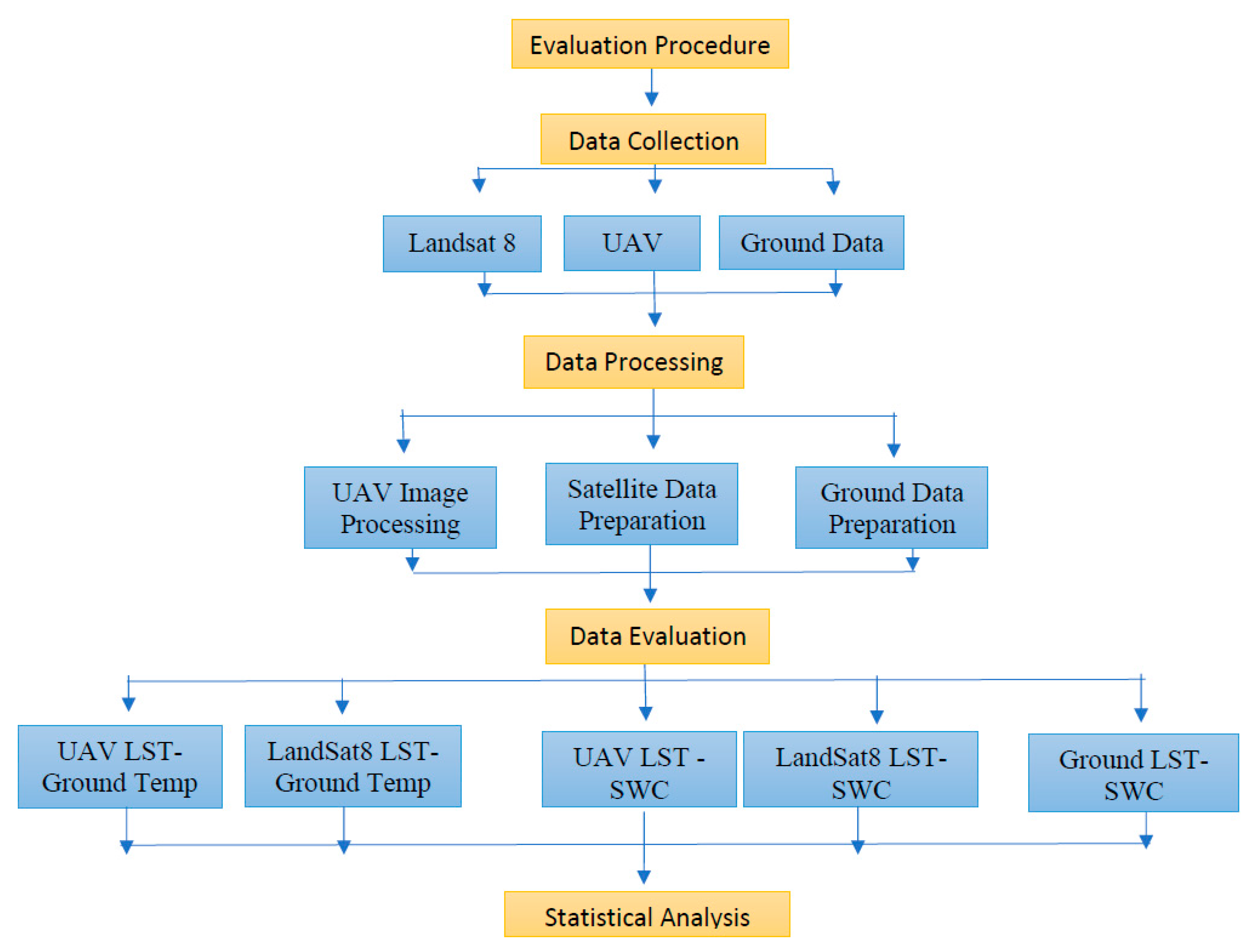
2. Materials and Methods

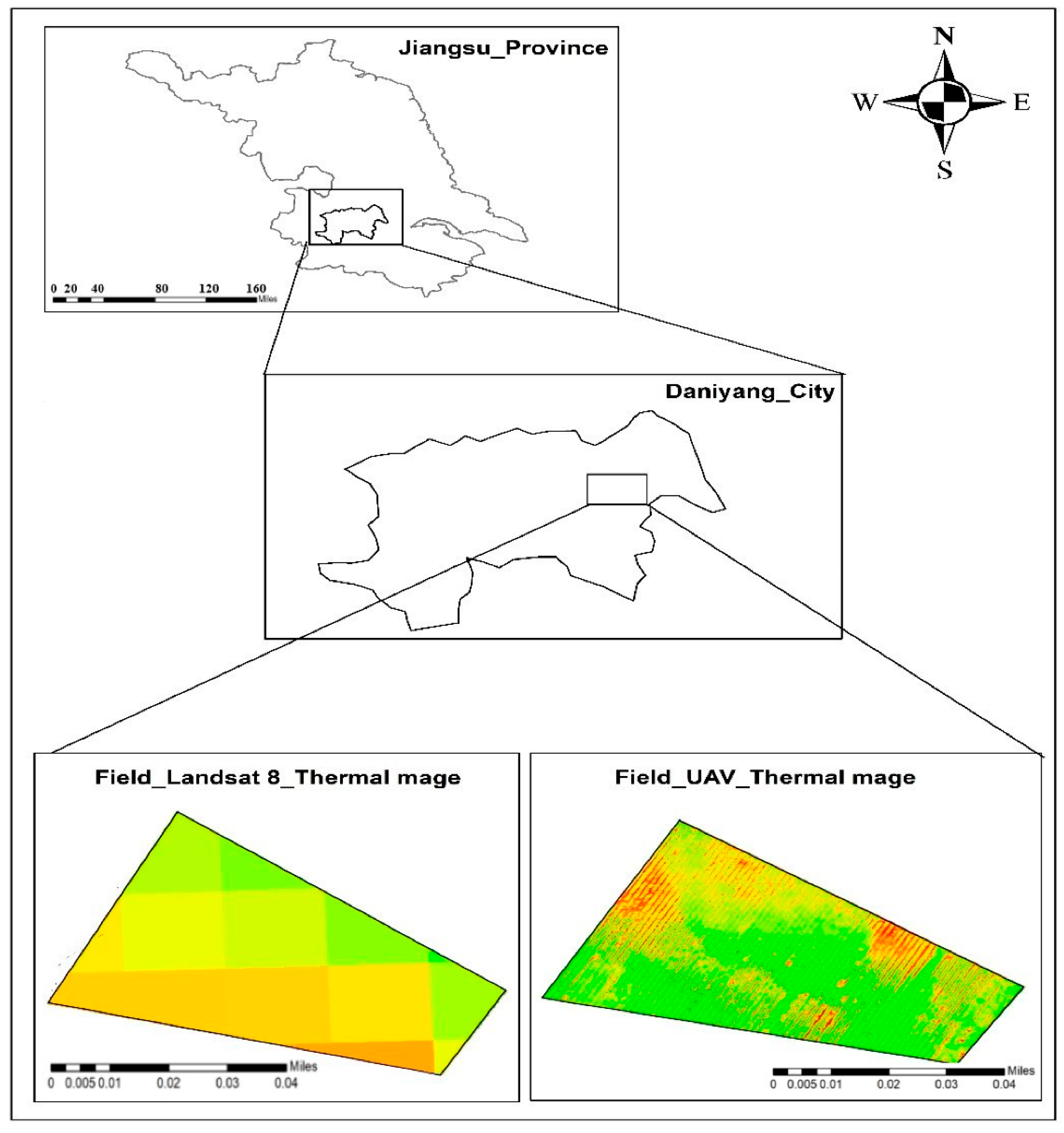
2.1. Study Site

This research was carried out in a tea farm on cultivated land at Danyang (32°1′00″ N, 119°4′00″ E) in the 5-acre tea field about 60 km from Zhenjiang City, Jiangsu Province, China, with an elevation of 18.5 m above the sea level (Figure 1). A detailed discussion about the study site has been discussed in our previous research [9]. This site was chosen because (a) it offers diversity in terms of tree species composition, (b) it has easy access, (c) it is large enough to be imaged by several Landsat pixels, and, most importantly, (d) it allowed repeated UAV flights to be undertaken with minimal risk, as safety is paramount in UAV operations. Ground and UAV data were collected during the experiment duration. The texture of the field soil was silty-loam. Most of the instruments were deployed in the center of the study field on a flux tower to ensure the prevailing wind direction created the most significant footprint. The experiment was conducted on 18 August (230 DOY) and 2 September (DOY 245) 2020. The experimental land’s soil surface was shaded by the geotextile mulch and the tea canopies themselves. Similar tea fields neighbored the functional area with some trees on the southern and westerly field boundaries. Evaporation losses were assumed to be negligible. A meteorological station was set up on a 12 m tall tower (made of aluminum) that was placed in the study site with a maximum available fetch of 175 m in the dominant wind direction. This tower was for supporting all the necessary instrumentation that were used during the experiment. The soil temperature was measured using a sensor (TCAV-L, Campbell Scientific, Logan, UT, USA). Other parameters, including relative humidity and the air temperature, were measured using a sensor (HC2S3-L, Campbell Scientific., Logan, UT, USA). All the instrumentations that were used in the present study are presented with manufacturers and installation height (

Table 1. Instruments that were used during the experiment.

Sensors Items	Notation	Units	Height (m)	Equipment, Type, and Manufactures
Soil water content (SWC)	θv	m3·m−3	0.04 (Depth)	CS655, Campbell Scientific Inc., Logan, UT, USA.
Soil temperature (ST)	Tsoil	°C	0.02 and 0.06 (Depth)	TCAV-L, Campbell Scientific, Logan, UT, USA.
Air temperature	Ta	°C	1.8	Fine-wire thermocouple, COCO-002, Omega, Eng., Sittingbourne, Kent UK.
Liquid precipitation	-	m·m	2.1	TE525MM, Campbell Scientific Inc., Logan, UT, USA.
Wind velocity, Sonic temperature	u,v,w Ts	m·s−1 °C	2.3	CSAT3, Sonic anemometer, Campbell Scientific, Logan, UT, USA.
Relative humidity	RH	%	2.1	HC2S3-L, Campbell Scientific, Logan, UT, USA.
Net radiation	Rn	W·m−2	2.3	CNR4-LKIPP and Zenon.

).

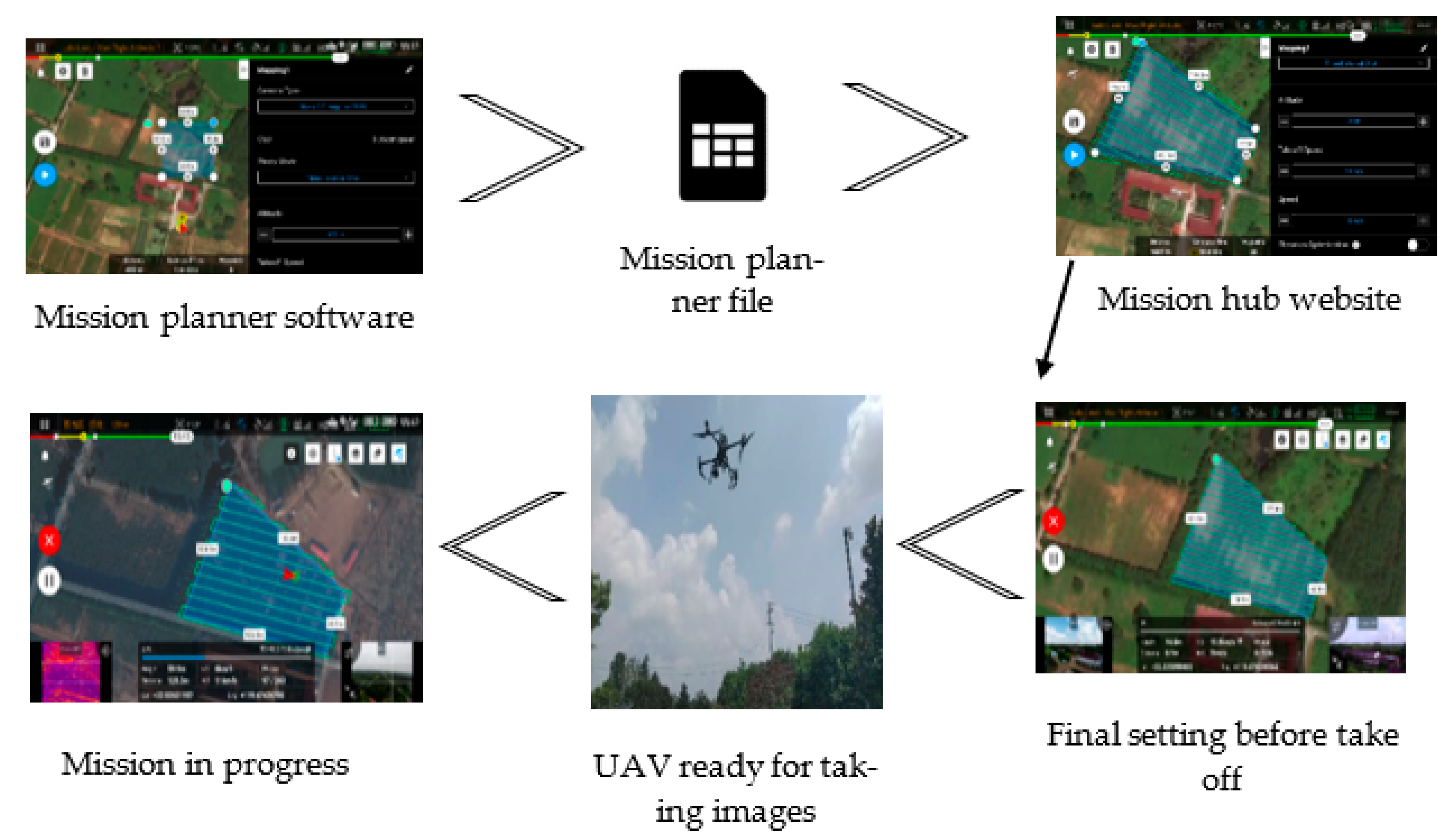
2.2. UAV Data Acquisition

The collection, processing, calibration, and validation of the UAV data series in this study are described in detail in our previous literature [9]. The UAV TIR images were captured on DOY 230 and 245, when the shadow influence was negligible due to the maximum solar altitude. A total of 14 random GCPs were measured across the experimental field and the coordinates were measured with a total accuracy of 0.1 m using GNSS (Global Navigation Satellite System). The flights were planned for sunny days with good visibility and a moderate wind level. The flight was at the height of 60 m. The image–image overlapping ratio was set to 85%. The Pix4D Mapper program was used to create orthoimages from the collected images with a spatial resolution of 0.2 cm. The image collection missions were produced using the DJI A3 flight controller on the Mission Planner with DJI Ground Stations Pro software (SZ DJI Technology Co. Ltd., Zhenjiang, China), as shown in (Figure 2).

Table 2. The detailed specification of UAV and sensor used for the experiment.

Item	Detailed Specification
DJI (M300 RTK)	Exposure mode: Auto, Manual Weight: 2.7 kg Flight time: 55 min Scale range: −400 to 1500 °C Frame rate: 30 Hz Pixel pitch: 12 µm ISO Range: Video: 100–25,600 Take-off weight: 9 kg
Zenmuse XT 2 FLIR	Digital Zoom: 1×, 2×, 4×, 8× Thermal sensitivity: ≤50 mk @ f 0.1 Spectral band: 8–14 µm Exposure Compensation: ±3.0 (1/3 increment) Lens: FOV:40.6.0 Resolution: 640 × 512 pixels Photo format: R-JPEG (16 bit)

shows the precise specifications of the instruments that were utilized to capture the photos. The LST was measured in the Pix4D mapper program using he following equation: the long-wave radiance was obtained from FLIR software.

UAV LST °C = Longwave radiance × 0.04 − 273.15

(1)

2.3. Satellite and Aerial Remote Sensing Data

The TIR sensor on the Landsat 8 satellite can estimate LST with an image resolution of 100 m and a chronological revisit of 16 days in two frequency TIR bands (10 (10 m) and 11 (12 m). The data for the sample area were collected from the United States Geological Survey website (https://earthexplorerrer.usgs.gov) on 18 August (230 DOY) and 2 September (DOY 245) 2020, and was sourced from the Landsat 8 Operational Land Imager (OLI)/Thermal Infrared Sensor (TIRS) sensors. The photos were taken with clear-sky scenes of the experimental area and processed according to [27] on the same days of UAV flight as DOY 230 and DOY 245 2020.

Table 3. The detailed specification of the Landsat 8 satellite and sensor.

Item	Detailed Specification
Landsat 8 Satellite	Weight: 2071 kg Temporal revisit: 16 days Band 10: TIRS 1 (10.6–11.19 µm) 100 m Band 11: TIRS 2 (11.5–12.51 µm) 100 m Length: 3 m Diameter: 2.4 m Equatorial crossing time: 10:00 a.m. +/−15 min
Landsat 8 sensor	Output format: Geo TIFF Pixel value: 16-bit pixel Accuracy: 41 m circular error, 90% confidence Orbit angle: Inclined 98.2° Spatial resolution: 100 m Accuracy: spatial resolution +/−1 percent

shows the Landsat 8 sensor satellite’s detailed specifications. The Landsat sensor passes over Danyang City between 02:31 and 02:40 GMT, which is 10:31 to 10:40 am local time. ERDAS Imagine 9.1 and ArcGIS 9.3 were used to do the image processing. The statistical analysis was calculated using MS-Excel and Origin applications. The Landsat images must be pre-processed to perform a geometric correction for the Landsat level 1 product since they are recorded and ortho-rectified systematically. As a result, the primary correction that is needed is radiometric. The radiometric correction corrects errors that impact the pixel brightness values. These errors are mainly caused by sensor device recognition and ambient attenuation errors. Since the initial image sizes are more significant than the sample area, they are edited using a shapefile of the experimental field after pre-processing. The thermal bands of the Landsat data sets were used to extract LST.

2.4. Retrieving LST Algorithm from Landsat Data

The data collection for the LST from Landsat 8 TIRS, both bands 10 and 11 consists of the reversal of radiative transfer equation (RTE), which is used to correct for the top of atmosphere (TOA). The RTE for a single TIR band is expressed as;

$${\mathsf{L}}_{\mathsf{T}\mathsf{O}\mathsf{A},\mathsf{i}}=\left[{\mathsf{\epsilon }}_{\mathsf{i}}{\mathsf{\beta }}_{\mathsf{i}}\left(\mathsf{L}\mathsf{S}\mathsf{T}\right)-\left(1-{\mathsf{\epsilon }}_{\mathsf{i}}\right){\mathsf{L}}_{\downarrow \mathsf{h}\mathsf{e}\mathsf{m},\mathsf{i}}\right]{\mathsf{\tau }}_{\mathsf{i}}+{\mathsf{L}}_{\uparrow \mathsf{a}\mathsf{t}\mathsf{m},\mathsf{i}}$$

(2)

where, L_TOA,i is the TOA radiance that is measured by the TIR sensor, εi was used to represent the surface emissivity; β_i is the blackbody emitting the surface temperature, and L_↓hem,i, τi, and L_↑atm,i are the atmospheric features, atmospheric transmissivity, and up-welling radiance, respectively. In the RTE, the subscript i denotes the active channel quantity of all the parameters in bands 10 and 11. The L_{TOA i} was used to determine the digital number (DN) with the conversion to text it from band 10 and 11 of the TIR bands at radiance [28]:

$${\mathsf{L}}_{\mathsf{T}\mathsf{O}\mathsf{A},\mathsf{i}}=0.0003342\ast \mathsf{D}\mathsf{N}+0.1$$

(3)

$$\begin{array}{l}\mathsf{L}\mathsf{S}\mathsf{T}=\frac{{\mathsf{k}}_2}{\mathsf{ln}\left[\frac{{\mathsf{k}}_1}{{\mathsf{B}}_{\mathsf{i}}(\mathsf{L}\mathsf{S}\mathsf{T})}+1\right]}\\ \end{array}$$

(4)

For band 10, k₁ and k₂ are 774.89 Wm⁻² sr⁻¹ μm⁻¹ and 1321.08 K. The value for k_1, and k₂ for band 11 are 480.89 Wm⁻² sr⁻¹ μm⁻¹ and 1201.14 K respectively.

2.5. Single-Channel Algorithm

The single-channel algorithm (SCA) reprocesses the LST with the smallest critical input information using the proof for each TIR tube. However, only two SCAs were tested and validated in the Landsat 8 TIRS band 10.

$$\mathsf{L}\mathsf{S}\mathsf{T}=\mathsf{\gamma }\left[\frac{1}{{\mathsf{\epsilon }}_{10}}\left({\mathsf{\psi }}_1{\mathsf{L}}_{\mathsf{T}\mathsf{O}\mathsf{A},10}+{\mathsf{\psi }}_2\right)+{\mathsf{\psi }}_3\right]+\mathsf{\delta }$$

(5)

Here, ε₁₀ is the emissivity of the surface, and L_TOA,10 demonstrate TOA radiance, respectively. In addition, γ and δ are two constraints in Landsat8-TIRS band 10 and calculated by following equations as mentioned below:

$$\mathsf{\gamma }=\frac{{\mathsf{T}}_{10}^2}{{\mathsf{b}}_{\mathsf{r}}{\mathsf{L}}_{\mathsf{T}\mathsf{O}\mathsf{A},10}}$$

(6)

$$\mathsf{\delta }={\mathsf{T}}_{10}-\frac{{\mathsf{T}}_{10}^2}{{\mathsf{b}}_{\mathsf{r}}}$$

(7)

Here, T₁₀ denotes the sensor illumination temperature of band 10, and the value of bγ is equal to 121.47. The SCA that is projected by [29] approaches the atmospheric occupation Ψj with j = 1, 2, and 3. The second order polynomial fit is written as follows in matrix notation:

$$\left[\begin{array}{c}{\mathsf{\psi }}_1\\ {\mathsf{\psi }}_2\\ {\mathsf{\psi }}_3\end{array}\right]=\left[\begin{array}{ccc}0.04019& 0.02916& 1.01523\\ -0.38333& -1.50294& 0.20324\\ 0.00918& 1.36072& -0.27514\end{array}\right]\left[\begin{array}{c}{\mathsf{W}}^2\\ \mathsf{W}\\ 1\end{array}\right]$$

(8)

Here, the second SCA that was endorsed in the research was predictable by Wang et al. [30]. This approach implements the LST equation.

$$\mathsf{L}\mathsf{S}\mathsf{T}=\frac{\left[{\mathsf{a}}_{10}\left(1-{\mathsf{C}}_{10}-{\mathsf{D}}_{10}\right)+\left({\mathsf{b}}_{10}\left(1-{\mathsf{C}}_{10}-{\mathsf{D}}_{10}\right)+{\mathsf{C}}_{10}+{\mathsf{D}}_{10}\right){\mathsf{T}}_{10}-{\mathsf{D}}_{10}{\mathsf{T}}_{\mathsf{a}}\right]}{{\mathsf{C}}_{10}}$$

(9)

The real mean atmospheric temperature is T_a, and the regression coefficients are dependent on a₁₀ and b₁₀ inside the T₁₀ range. For the Landsat 8-TIRS band 10, these were utilized to determine the Planck radiance imitatively.

Table 4. The Landsat 8 TIRS band 10 coefficients a10 and b10 [30].

Temperature Range (°C)	a10	b10	R2
50–70	−70.1775	0.4581	0.9997
30–50	−62.7182	0.4339	0.9996
−20–30	−55.4276	0.4086	0.9996

displays the values of these coefficients in the T₁₀ ranges.

The outside parameters for the algorithm are C10 and D10, which are determined using the following equations:

$${\mathsf{C}}_{10}={\mathsf{\tau }}_{10}{\mathsf{\epsilon }}_{10}$$

(10)

$${\mathsf{D}}_{10}=\left(1-{\mathsf{\tau }}_{10}\right)\left[1+\left(1-{\mathsf{\epsilon }}_{10}\right){\mathsf{\tau }}_{10}\right]$$

(11)

The atmospheric transmissivity that is filtered for the Landsat 8 TIRS band 10 is represented by the τ₁₀.

2.6. Comparison of UAV TIR LST with Satellite LST

The UAV TIR LSTs for the measurement points were correlated to the Landsat 8 LST to ensure accuracy. At the measurement points, the UAV TIR LSTs were calculated and their difference from the observed values was studied. The methodologies that were employed were the root-mean-square error, linear regression analysis, and scatter plot analysis. The daily average UAV TIR LST was determined and the RMSE of the measured values was examined. The assessment process is detailed in the flow chart below (Figure 3).

3. Numerical Analysis

A statistical analysis approach was used to compare the UAV TIR LST with the Landsat 8 TIR LST and in situ observations. When compared to ground stations, these models explain inaccuracies in the UAV data. Comparisons were made using the same linear regression equation; root-mean-square error (RMSE), mean absolute error (MAE), relative bias (RB), coefficient of correlation (CC), and the coefficient of determination (R²). As shown in the equations below (

Table 5. Statistical measures.

Statistical Model Name	Equation	Applications
Root-mean-squared error (RMSE)	$\sqrt{\frac{1}{\mathrm{n}}{\displaystyle \sum _{\mathrm{i}-1}^{\mathrm{n}}}\left|\mathsf{Xi}-\mathsf{Yi}\right|}$	The express error between UAV and satellite data
Mean absolute error (MAE)	$\frac{1}{\mathrm{n}}{\displaystyle \sum _{\mathrm{i}-1}^{\mathrm{n}}}\left|\mathsf{Xi}-\mathsf{Yi}\right|$
Relative Bias (RB)	$\frac{\frac{1}{\mathrm{n}}{{\displaystyle \sum }}_{\mathrm{i}-1}^{\mathrm{n}}\left(\mathsf{Xi}-\mathsf{Yi}\right)}{{{\displaystyle \sum }}_{\mathrm{i}-1}^{\mathrm{n}}\mathsf{Yi}} \times 100$	Describe the extent of agreement between satellite and gauges
Coefficient of correlation (CC)	$\frac{\frac{1}{\mathrm{n}}{{\displaystyle \sum }}_{\mathrm{i}-1}^{\mathsf{n}}(\mathsf{Xi}-\overline{\mathsf{X})} (\mathsf{Yi}-\overline{\mathrm{Y})}}{{\mathsf{\sigma }}_{\mathrm{x}}{\mathsf{\sigma }}_{\mathrm{y}}}$
Coefficient of determination (R2)	$1 - \frac{{\mathsf{SS}}_{\mathsf{regression}}}{{\mathsf{SS}}_{\mathsf{Total}}}$

), these indicators have been determined.

4. Results and Discussion

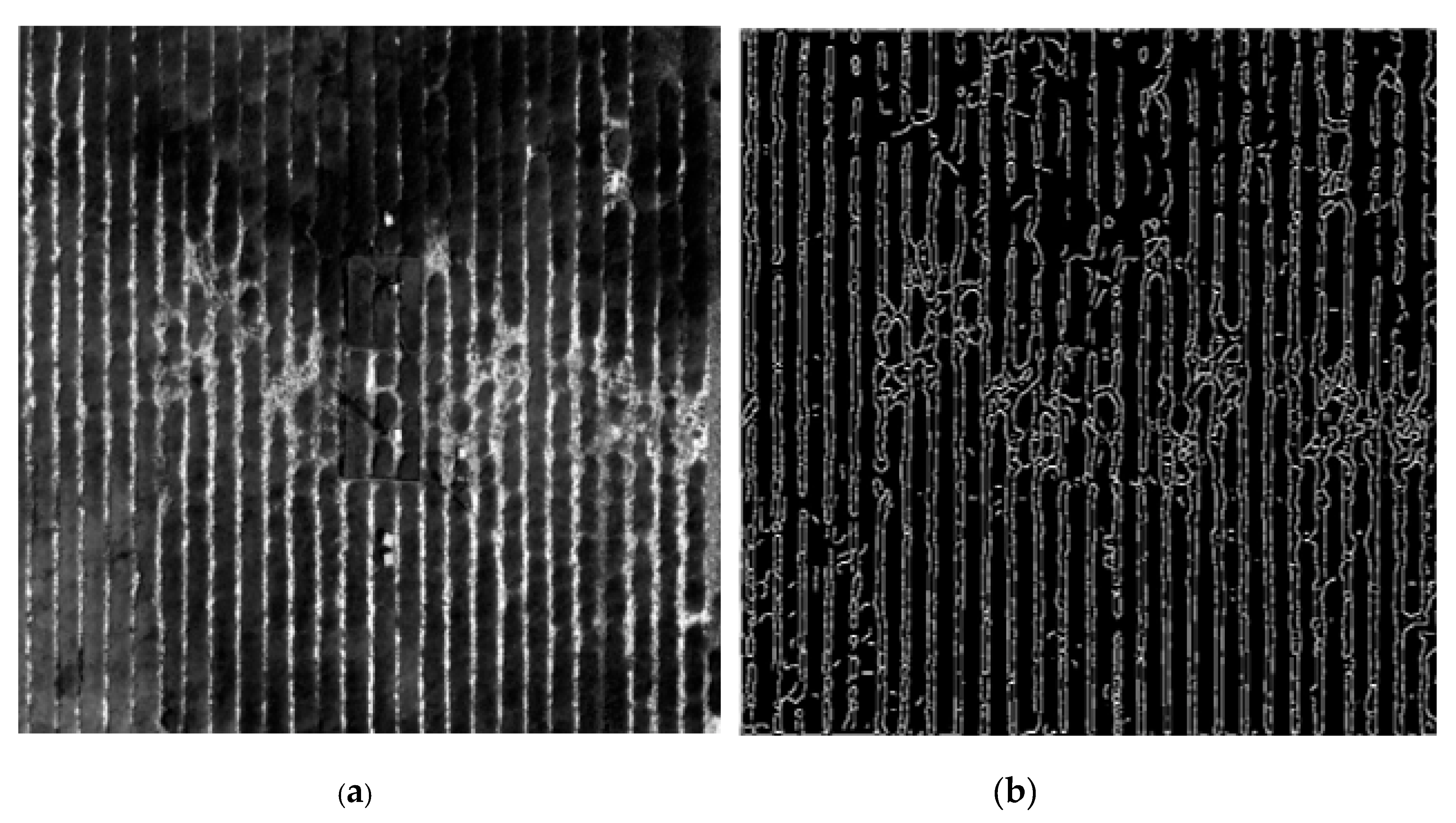
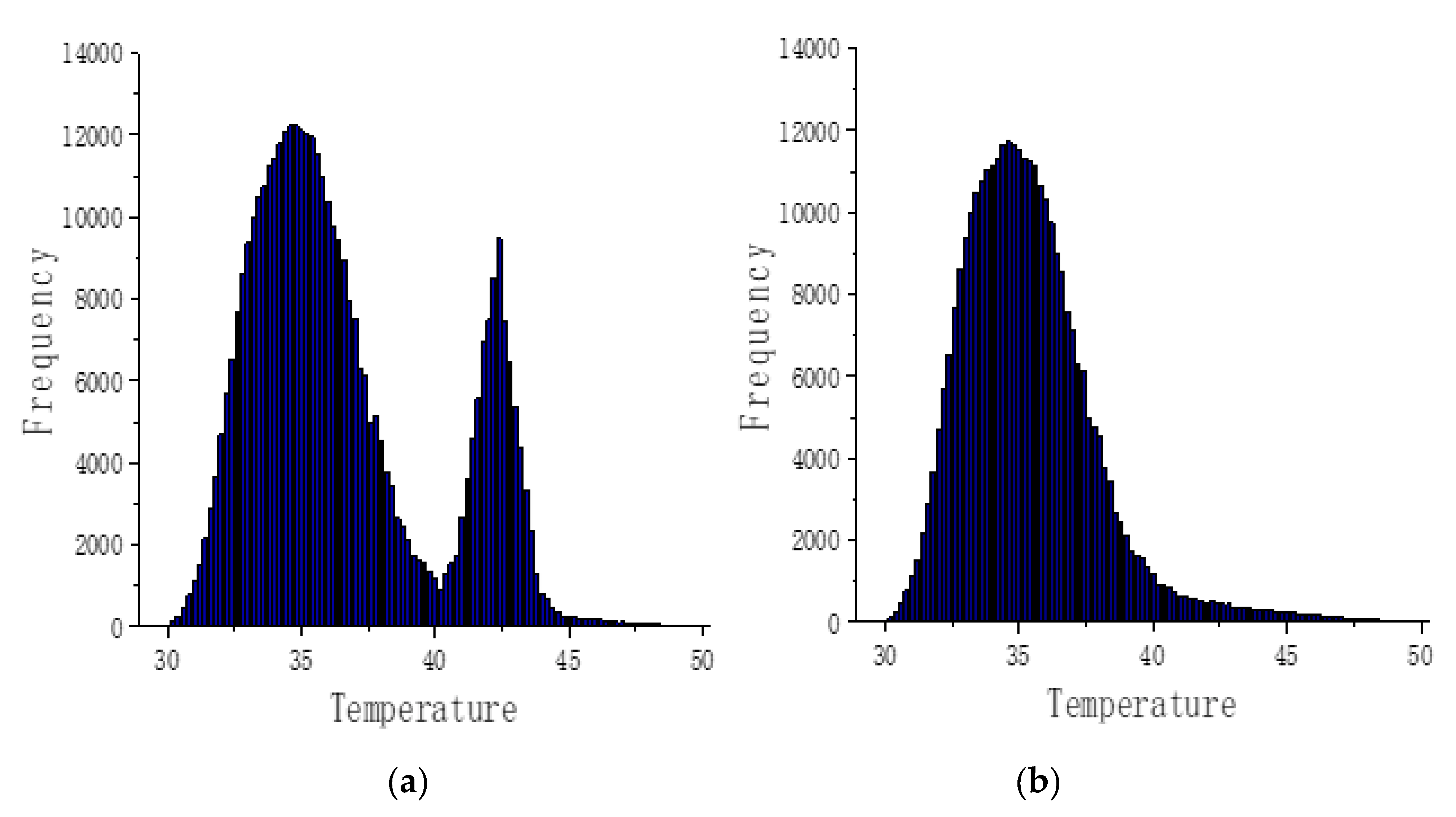
4.1. Soil Background Removal Validation

The purpose of removing the soil background is to reduce the reflectivity of the soil background and obtain accurate canopy temperature data [31]. The Canny edge detection algorithm removed the soil background of the infrared thermal images of the farmland study area. The edge detection result of the denoised infrared thermal image using the Canny edge detection algorithm is shown in Figure 4. It can be seen that the Canny edge detection algorithm can accurately identify the boundary pixels between the crop canopy and soil background.

4.2. Histogram Analysis of Removal of Soil Background Temperature

To further illustrate the effect of the Canny algorithm on removing soil background, Figure 5 shows the temperature histogram of the raw infrared thermal images and the infrared thermal images by the Canny edge algorithm, respectively. The soil pixel and crop canopy pixel represent two different material types. Different material types have a different radiance to temperature so the extracted temperature values are also different. It can be seen from Figure 5a, that the temperature histogram of the raw infrared thermal image is a bimodal shape, the pixel temperature values that are occupied by the first peak are lower, and the material type is crop canopy. The pixel temperature values that are occupied by the second peak are higher, so the material type that is represented is soil background. The Canny method in this paper was used to eliminate the second peak. The single peak shape of the temperature histogram can determine that the soil background has been eliminated. It can be seen from Figure 5b that the temperature histogram after removing the soil background by Canny presents an obvious single peak shape. The histogram roughly obeys the normal distribution law, and its contour is smooth.

4.3. Histogram Analysis of Removal of Soil Background Temperature

The accuracy of the raw infrared thermal images and the infrared thermal imaging by Canny to predict the canopy temperature is shown in Figure 6a,b. By linearly fitting the canopy temperature data that were extracted from the images with the real ground canopy temperature data, it was found that the fitting degree between the canopy temperature data that were extracted by the Canny method and the real ground canopy temperature data ($R^2$ = 0.9355) was significantly higher than that of the raw images ($R^2$ = 0.7673). By applying the Canny method, the extraction accuracy of target canopy temperature data can be improved. In this respect, our research has the same result as the literature [32]. Therefore, infrared thermal imaging that eliminates the soil background can extract the target canopy temperature data.

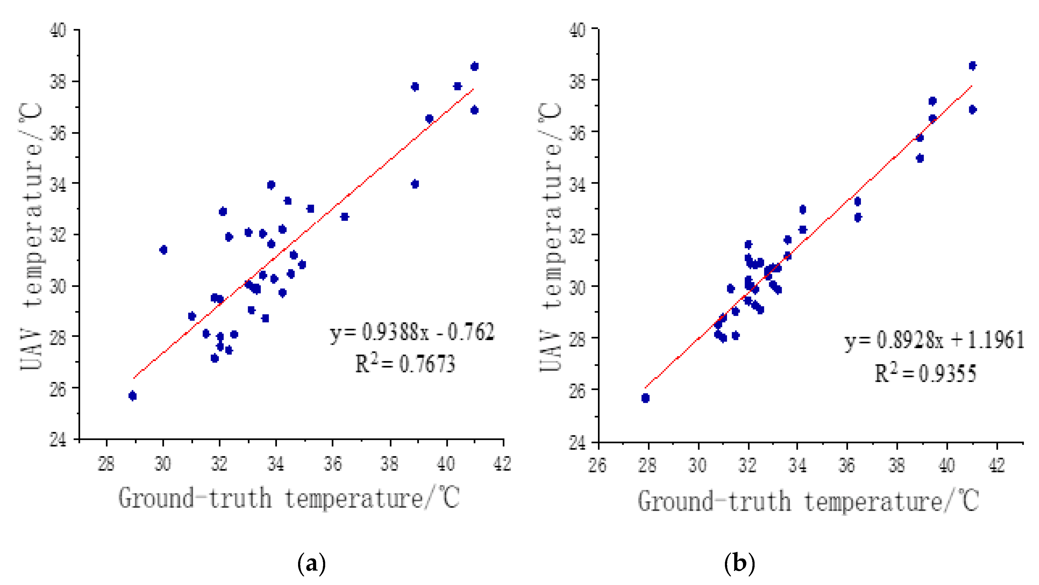
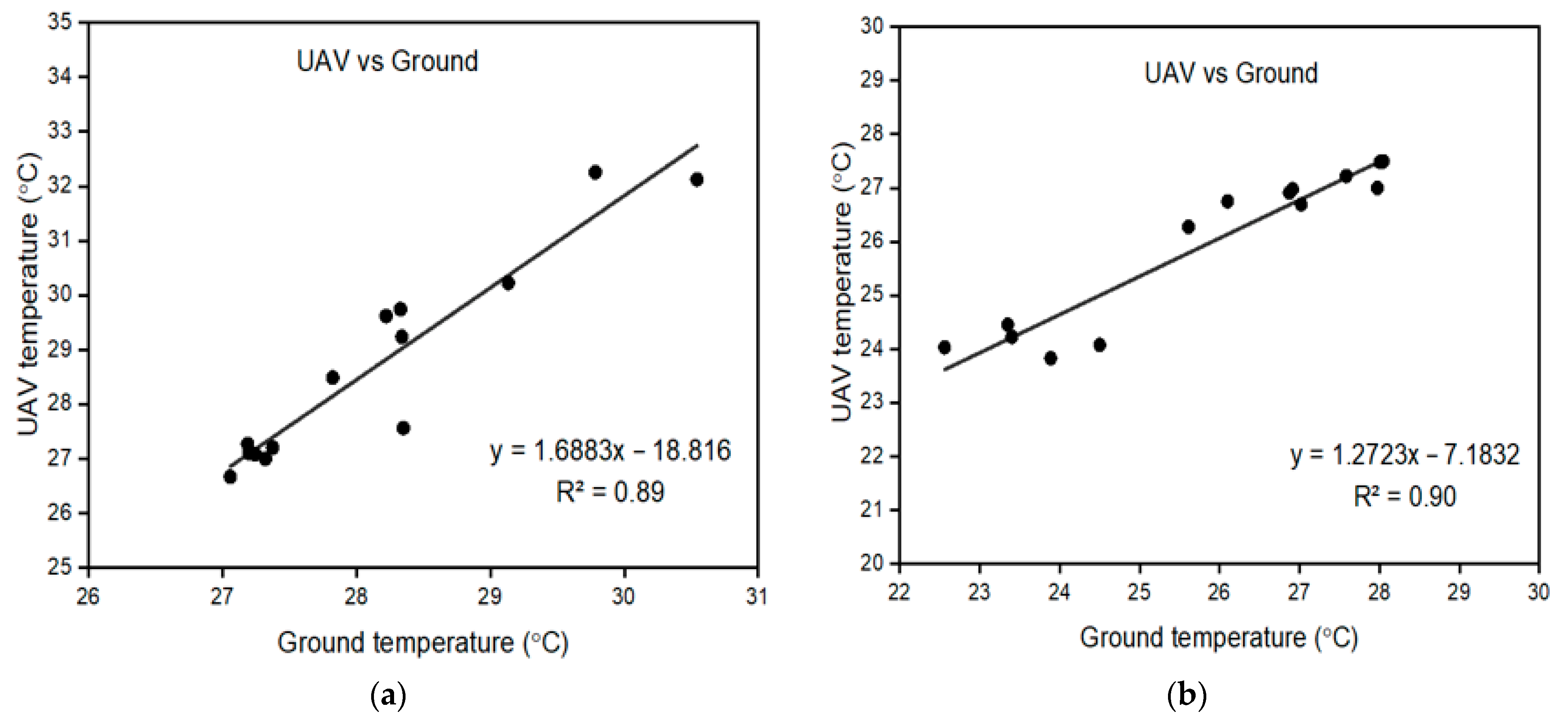
4.4. UAV-Ground LST Validation

The validation study that is proposed here shows the comparison of LST that was estimated by the UAV and ground truth measurement. These algorithms have in situ values that were measured from a nearby weather station where the UAV was flown and capturing images. For this study, the UAV-mounted thermal infrared (TIR) sensor was operational for the two days when the satellite reading was available. After 40 min of flight, the TIR images were captured and later on were processed as discussed in Section 2.2. A relatively higher temperature was observed on DOY 230 of 2020 than the images of DOY 245. The maximum difference of approximately 3 °C was found on both days, and variation in this temperature was due to the weather conditions and higher soil moisture due to rainfall. As fields had the same type of crop at the time of fight, no land cover effect was taken. The entire weather station setup was situated inside the field to measure the metrological parameters, including air temperature, humidity, and solar radiation, etc., as mentioned in

Table 6. Mean values of the weather parameters that were registered on the sampling days.

Experiment (230 DOY)				Experiment (245 DOY)
Tair (°C)	RH (%)	VPD (KPa)	Wind Speed (m/s)	Tair (°C)	RH (%)	VPD (KPa)	Wind Speed (m/s)
16.8	64	0.78	0.5	24.5	67	1.04	0.4
26.6	57	1.59	1.7	29.5	61	2.45	0.9
36.5	52	3.90	1.9	34.4	57	3.85	1.5
36.5	50	2.98	1.8	35.9	53	2.90	1.8
37.2	46	2.10	1.8	34.6	48	2.45	1.7

.

The soil temperature from the ground was observed at 14 points of the field for making a comparison with the TCAV-L temperature. The maximum soil temperature on DOY 230 was 27.4 °C, while a minimum of 23.8 °C was found. On the other hand, the maximum soil temperature on DOY 245 was 30.54 °C, while the minimum was 27.0 °C. UAV sensors also detected the land surface temperature with high resolution and were later combined to make a whole field mosaic. Each day provides a diverse range of temperatures with a maximum of 32.2 °C on DOY 245. A regression and correlation were compared between the ground- and the UAV-captured images on DOY 230 (Figure 7a). The results that were obtained from this study highlighted the promising results of the UAV-TIR images with in situ measurements. On 18 August, regression analysis between the UAV and the ground data provided the substantial value of R² (0.89), indicating best fitting with the actual data. The correlation coefficient was also 0.94, describing the greater extent of agreement between the ground and the UAV measurements.

Many previous studies have proven the same results [33,34,35]. The root-mean-square (RMSE) and the mean absolute error (MAE) were calculated to estimate the degree of error between the readings. In RMSE, values reached 1.07 °C, while for MAE, it captured a value of 0.82 °C, describing the fluctuation of error that was much lower (<1). Similarly, the data have been passed through a bias calculation to get an idea about under and overestimating temperature. The results suggested the BIAS for UAV was −0.49, and the negative sign indicated the underestimation of data by the UAV; however, this value was much less and did not affect the UAV observation performance (

Table 7. Statistical performance of the UAV with ground measurements.

Comparison	DOY	R2	RMSE	MAE	BIAS	CC
UAV vs. Ground	230	0.89	1.07	0.82	−0.49	0.94
	245	0.90	0.70	0.57	−0.13	0.95

). Similar performance measures were applied to the second day of observation DOY 245, which gave approximately the same results. Regression analysis and correlation coefficient provided higher values, 0.90 and 0.95, respectively, indicating a greater extent of the agreement, as shown in Figure 7b. Also, parameters of error (RMSE and MAE) showed a minor error in measurements of 0.70 °C and 0.57 °C, respectively, representing the lower degree of error. The bias value (−0.13) also indicated the underestimation behavior with the field data. The UAV-TIR images performed very well either in regression, correlation, or LST estimation error.

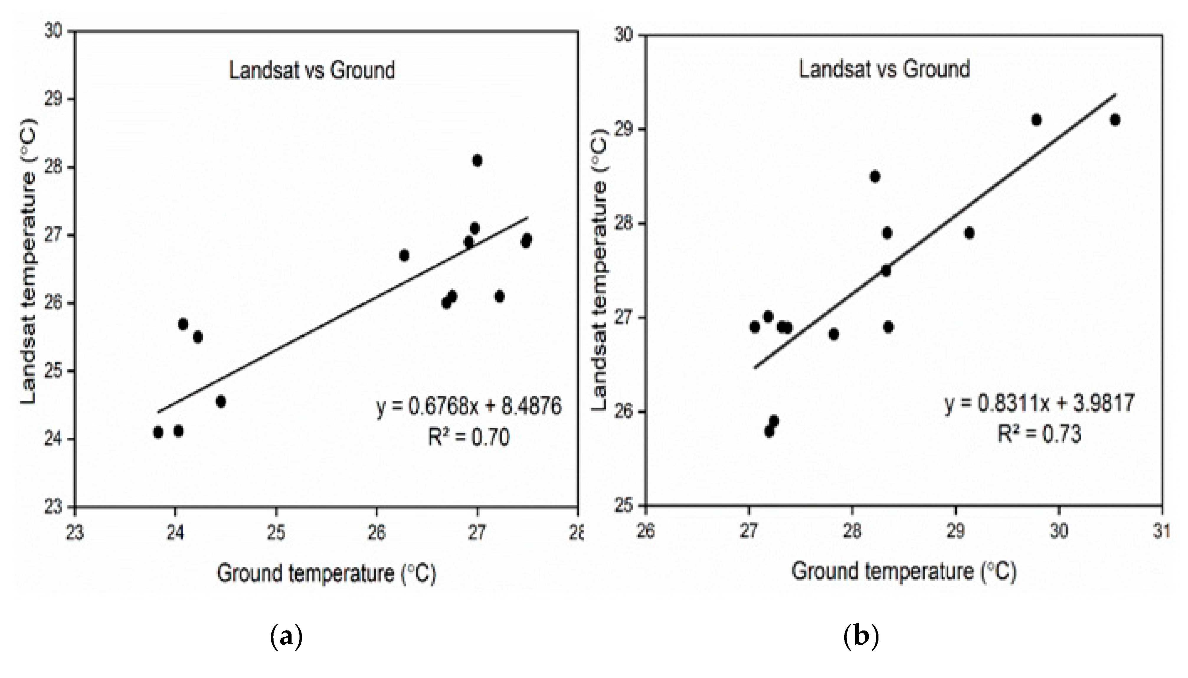
4.5. Landsat-Ground LST Validation

Table 8. Statistical performance of Landsat 8 with ground measurements.

Comparison	DOY	R2	RMSE	MAE	BIAS	CC
UAV vs. Ground	230	0.70	0.78	0.62	0.08	0.83
	245	0.73	0.94	0.81	1.11	0.85

shows the ground and Landsat 8 LST validation comparison results. The ground data was measured by the TCAV-L instrument, which was used to validate and evaluate the Landsat LST retrieval algorithm. When comparing the LST results to the ground measurements, there may be a 5 °C difference. The accuracy of the results in certain places was within 2 °C of the actual ground temperature that was proposed by Srivastava et al. [36]. As the resolution of Landsat 8 for the used band was 100 m for the thermal band, the comparison was made with the in-situ data, which is different and can often result in large variations. The extent of agreement, regression, and correlation were found for observation day. Hourly data were obtained from a local weather station and compared to the retrieved LST. Images from the satellite were downloaded based on the information that was available. One satellite image was downloaded on each of the two days (DOY 230 18 August and DOY 245 2 September). A total of two satellite images from two different dates were selected based on data that were available to compare the findings. For DOY 230, regression analysis indicated moderate results (R² = 0.70) with the in-situ data, as shown in (Figure 8a). The correlation coefficient was 0.83 and showed a better relationship of both data. Similarly, in RMSE and MAE, 0.78 °C and 0.62 °C values were observed, respectively, indicating a lower degree of error between both datasets. Approximately no bias (0.08) was observed for the Landsat data, showing no over- or under-estimation of the data. Similarly, the reading of DOY 245 also went through statistical measures and showed similar behavior. Regression and correlation provided 0.73 and 0.85 values, respectively, indicating an appropriate response to the ground data (Figure 8b). RMSE and MAE was found to be a little higher (0.94, 0.81) than previous observations (0.78, 0.62). However, Landsat 8 slightly over-estimated the readings as per the results of bias. Overall, the results indicated the lower performance of satellite than UAV measurements either in terms of errors or correlation. The reason for the better performance of UAV comes from the pixel size and distance from the Earth because, in the case of satellite, many parameters are involved which influence the temperature retrieval.

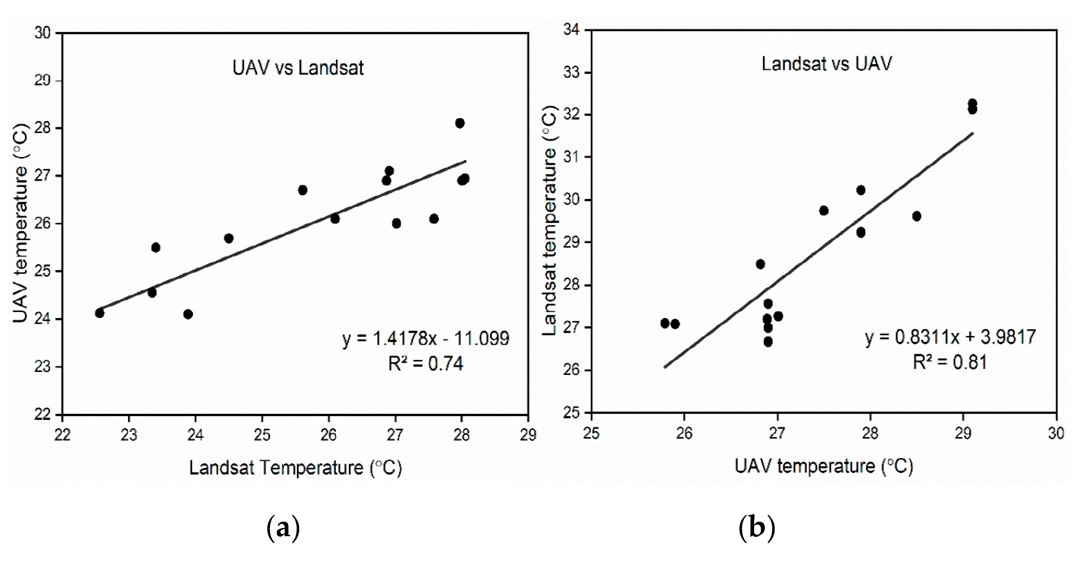
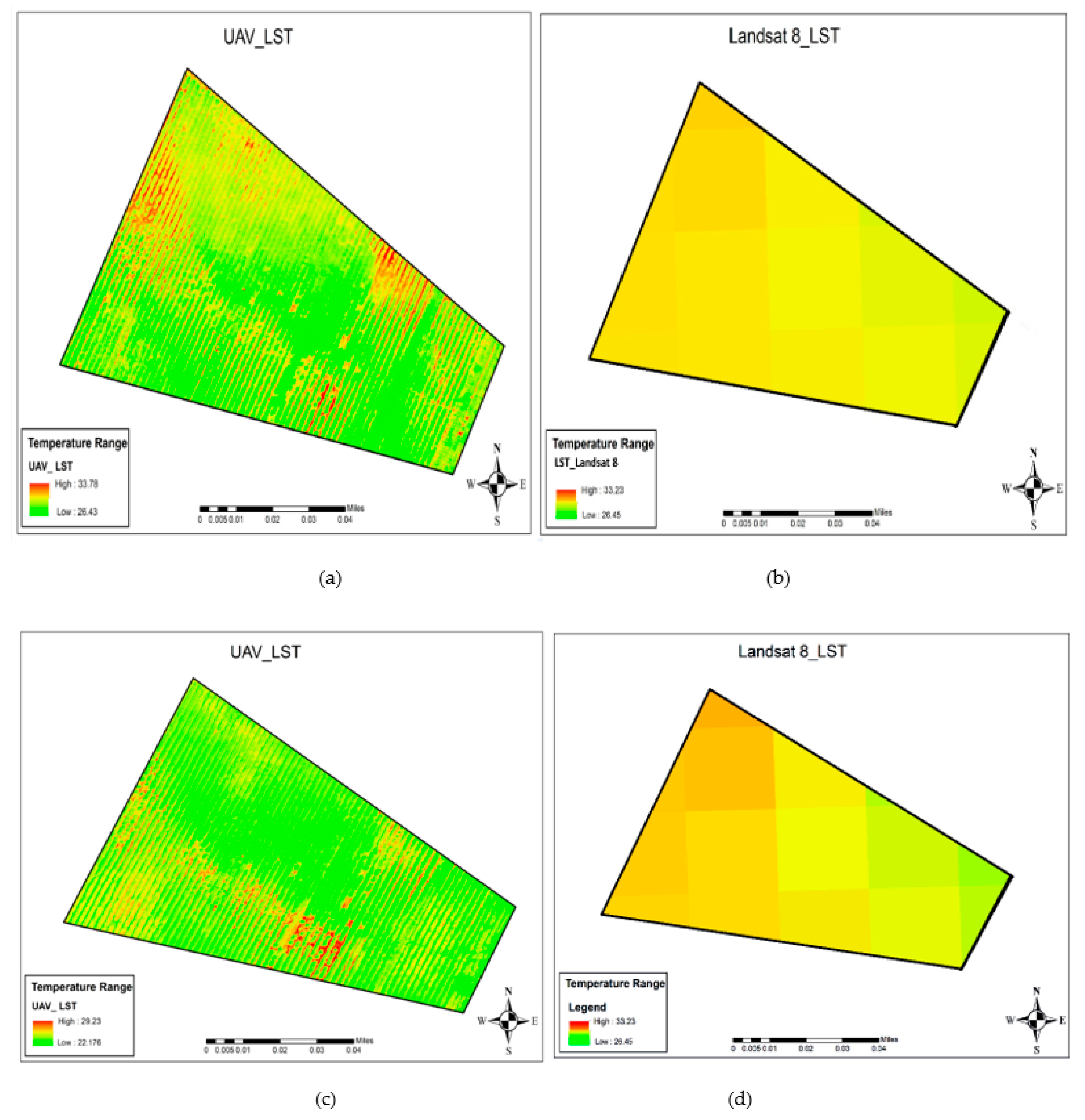
4.6. Landsat 8-UAV Data Retrieval Comparison

Landsat 8 and the UAV have thermal infrared sensors with their specific ranges as given in Table 2 and Table 3.

Table 9. Statistical performance of the UAV with Landsat 8 measurements.

Comparison	DOY	R2	RMSE	MAE	BIAS	CC
UAV vs. Landsat	230	0.74	1.09	0.25	0.08	0.85
	245	0.81	1.67	1.35	1.65	0.90

shows the comparison results of Landsat 8 and the UAV data retrieval. A comparative study was also taken under consideration to understand the detection relationship between both platforms. The temperature that was measured by Landsat 8 and the UAV was analyzed through statistical performance measures to find correlations between them. Based on the regression analysis (R² = 0.74) and correlation coefficient (0.85), a reasonable extent of agreement was detected for DOY 230 (Figure 9a). On the other hand, the results (R² = 0.81, CC = 0.90) that were attained on DOY 245 also showed promising results between both sensors (Figure 9b). The RMSE and MAE were found 1.09 °C and 0.89 °C for the reading of DOY 230, while it goes higher to 1.67 °C and 1.35 °C for DOY 245, respectively. The bias estimated that its value goes to a maximum of 1.65, indicating an overestimation for field area as shown below the table.

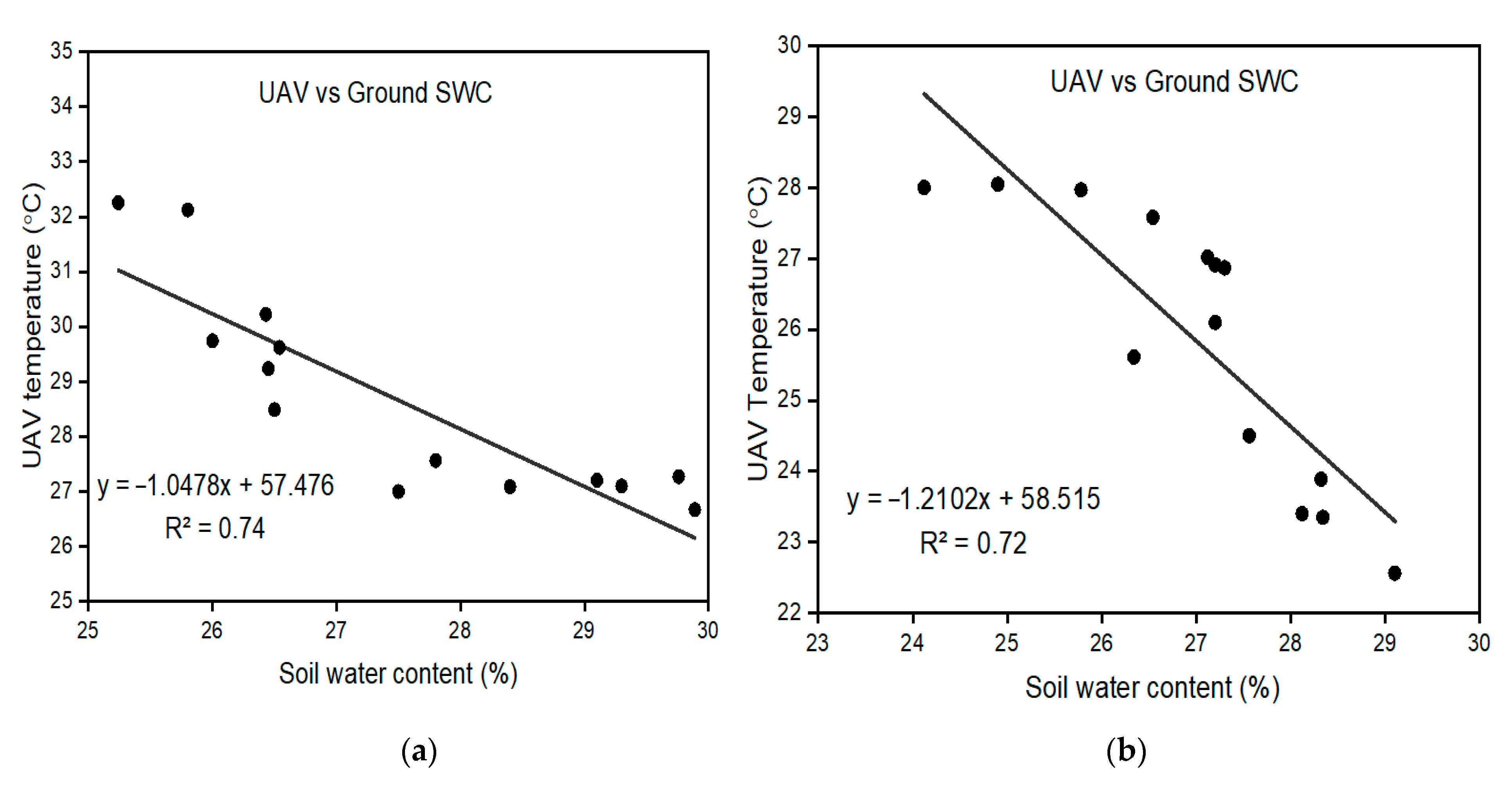
4.7. Relationship between UAV Retrieved LST and Soil Water Content

Soil moisture (SM) is an essential component of the Earth’s surface water balance, energy balance, and regulating the land surface temperature (LST). The relationship between LST and the available soil water content (SWC) was also observed. Thermal sensors with high resolution captured images by UAV help understand these variables relationships on a temporal basis. To understand the association between both quantities, regression and correlation were performed. The results suggested that the UAV-SMC correlation was negative (−0.85) for the image of DOY 230, while this value remained approximately constant (−0.86) for the DOY 245 as well (Figure 10a,b). The negative value indicates an inverse relationship between the moisture and soil temperature for a few hours per day. Previous studies in this field examined SM temporal evolution and reported its persistence for a few hours per day and even for a few days [37]. Points where the higher temperature represents lower moisture levels and lower temperatures have a higher moisture level. The results that were obtained by regression analysis were also suitable for UAVs ranging between 0.74–0.72, which also enforced the relationship between the variables.

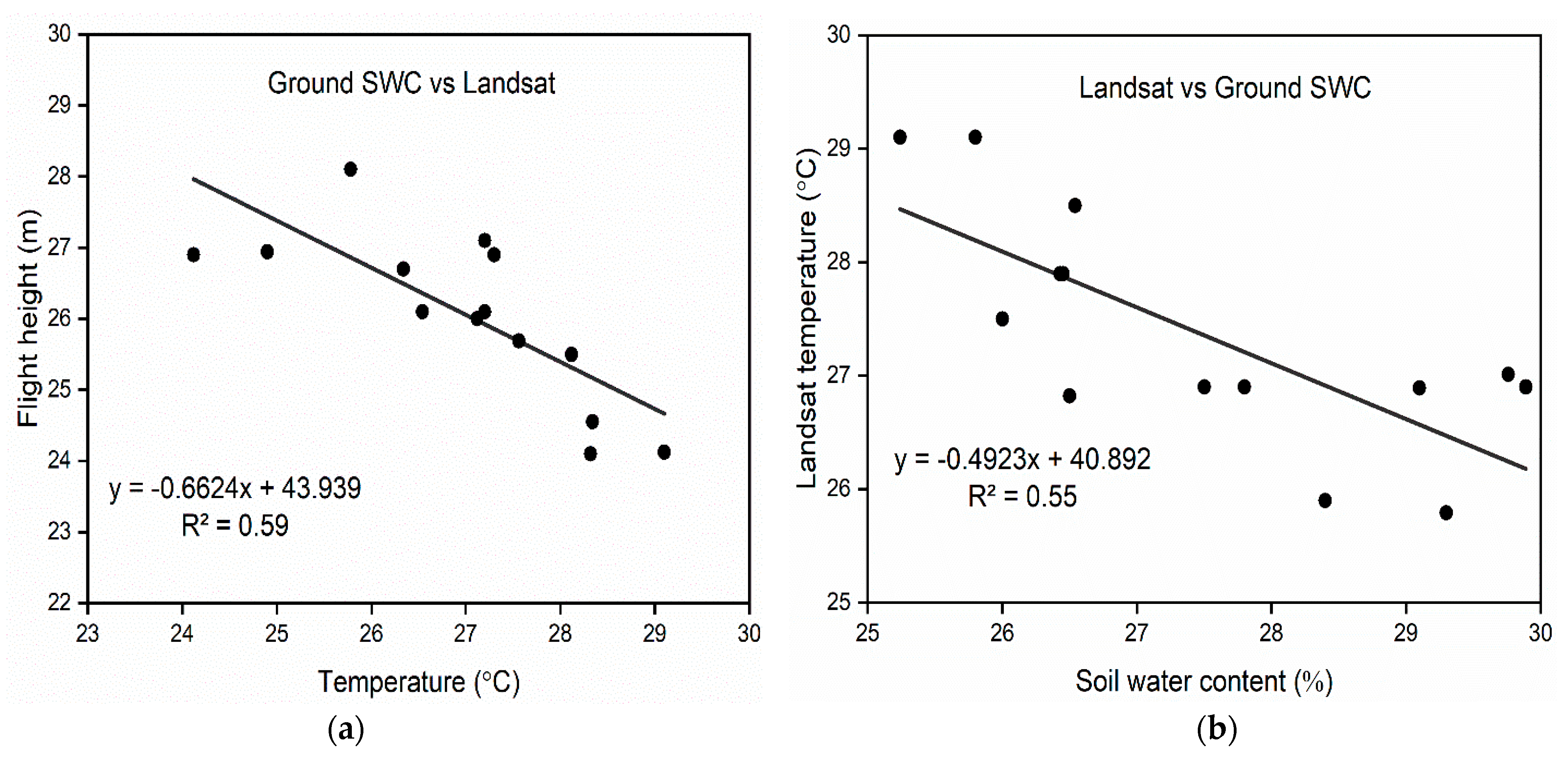
4.8. Relationship between Landsat 8 Acquired LST and Soil Water Content

The Landsat 8 satellite had the thermal band to capture high-resolution thermal images, which have been used in this study to estimate land surface temperature. Although the satellite images do not have as high a resolution as the UAV sensors, they provide satisfactory ground temperature results. Therefore, such a technique can be used for larger field areas. However, to understand the surface temperature retrieval ability of Landsat 8, the ground measurement was taken. Regression and correlation analysis were applied to both images to understand the relationship with soil water content (Figure 11a,b). The research showed a lower value of R² (0.59, 0.56) for both images, indicating a lower agreement of temperature detection with SWC. Likewise, the UAV negative correlation coefficient (−0.74, −0.76) showed an inverse relationship between both the variables. Although satellites do not perform much better than UAVs, they could be more promising for larger areas with less human resources and economic expenditure.

4.9. Accuracy Assessment of the UAV LST and Landsat 8 LST

To understand the detection accuracy of land surface temperature, performance measures were implemented over both platform images in which in situ ground data were used as a reference. The results showed that the UAV temperature detection ability was higher than Landsat 8 (Figure 12). Regression, correlation, and error estimation indicated the superiority of UAV over Landsat 8 in terms of temperature retrieval. Likewise, statistical measures of the soil moisture content with temperature were also dominant for the UAV over the satellite data. The difference in the sensor performance was due to numerous variables such as the instrument’s height, emissivity, and cloud interference. Another advantage of UAV was the pixel difference which can be seen in Figure 12a–d, showing the UAV and Landsat 8 images for the DOY 230 and DOY 245 more detailed information of field.

5. Conclusions

This research work is specifically useful for developing countries, where agriculture is the primary source of income. This study analyzed the UAV TIR LST and Landsat 8 TIR LST data and compared both the simulations with ground-truthing data. This objective also compares the detection ability of the Landsat-8 algorithm for the retrieval of land surface temperature as well as UAV thermal sensors for agricultural practices. In addition, we evaluated the accuracy of the UAV TIR LST and Landsat 8 TIR LST by calculating the in situ LST for each day. The development of UAVs and imaging sensor technologies makes it much easier to collect images with very high spatial and spectral resolutions. The Landsat 8 LST and UAV LST were acquired with the resolutions of 30 m and 0.90 m, respectively. The results that were obtained by statistical performance measures help to identify a better platform in this regard. Regression and correlation coefficients were developed to find the extent of agreement between the variables. When the accuracy of the UAV TIR LST and Landsat 8 TIR LST was compared using a linear regression analysis and RMSE calculations that were based on the measurement point of in situ LST, the UAV TIR LST demonstrated greater accuracy (R² 0.89, 0.90, root-mean-square error (RMSE) 1.07, 0.70 °C) than the Landsat LST accuracy (R² 0.70, 0.73, (RMSE) 0.78 °C). At the same time, the root-mean-square and mean absolute error were used to approximate the error in data retrieval. Ground measurements were used as a reference. The UAV data performed more accurately than Landsat 8, as evidenced by the higher degree of correlation and R². However, the error was found to be approximately the same for both platforms. Bias analysis revealed that Landsat 8 overestimated the temperature by approximately 1 °C while the UAV underestimated by half a degree. Observations of both the platforms were also analyzed mutually with each other, and as a result, good relationships were found. In future research employing UAV TIR LST in agricultural areas, the accuracy of UAV TIR LST might be enhanced by taking into account the impacts of the object’s emissivity, the UAV flying altitude, and the shooting angle of the thermal imaging camera on the accuracy of UAV TIR LST. The results of this study stated that the UAV TIR LST could be more reliable with a complex land cover field. This study’s results could be helpful in urban environmental design and planning for agricultural management.

References

1. Sellers, P.; Schimel, D. Remote sensing of the land biosphere and biogeochemistry in the EOS era: Science priorities, methods and implementation—EOS land biosphere and biogeochemical cycles panels. Glob. Planet. Chang. 1993, 7, 279–297. [Google Scholar] [CrossRef]
2. Song, K.; Zhou, X.; Fan, Y. Empirically Adopted IEM for Retrieval of Soil Moisture From Radar Backscattering Coefficients. IEEE Trans. Geosci. Remote Sens. 2009, 47, 1662–1672. [Google Scholar] [CrossRef]
3. Li, Z.-L.; Tang, B.-H.; Wu, H.; Ren, H.; Yan, G.; Wan, Z.; Trigo, I.F.; Sobrino, J.A. Satellite-derived land surface temperature: Current status and perspectives. Remote Sens. Environ. 2013, 131, 14–37. [Google Scholar] [CrossRef] [Green Version]
4. Berni, J.A.; Zarco-Tejada, P.J.; Suárez, L.; Fereres, E.; Sensing, R. Thermal and narrowband multispectral remote sensing for vegetation monitoring from an unmanned aerial vehicle. IEEE Trans. Geosci. Remote Sens. 2009, 47, 722–738. [Google Scholar] [CrossRef] [Green Version]
5. Awais, M.; Li, W.; Cheema, M.J.M.; Zaman, Q.U.; Shaheen, A.; Aslam, B.; Zhu, W.; Ajmal, M.; Faheem, M.; Hussain, S.; et al. UAV-based remote sensing in plant stress imagine using high-resolution thermal sensor for digital agriculture practices: A meta-review. Int. J. Environ. Sci. Technol. 2022, 1–18. [Google Scholar] [CrossRef]
6. Su, Z.B. A Surface Energy Balance System (SEBS) for estimation of turbulent heat fluxes from point to continental scale. In Proceedings of the Spectra Workshop, Noordwijk, The Netherlands, 12–13 June 2001; p. 23.1. [Google Scholar]
7. Awais, M.; Li, W.; Cheema, M.J.M.; Hussain, S.; AlGarni, T.S.; Liu, C.; Ali, A. Remotely sensed identification of canopy characteristics using UAV-based imagery under unstable environmental conditions. Environ. Technol. Innov. 2021, 22, 101465. [Google Scholar] [CrossRef]
8. Deilami, K.; Kamruzzaman, M.; Liu, Y. Urban heat island effect: A systematic review of spatio-temporal factors, data, methods, and mitigation measures. Int. J. Appl. Earth Obs. Geoinf. 2018, 67, 30–42. [Google Scholar] [CrossRef]
9. Awais, M.; Li, W.; Cheema, M.J.M.; Hussain, S.; Shaheen, A.; Aslam, B.; Liu, C.; Ali, A. Assessment of optimal flying height and timing using high-resolution unmanned aerial vehicle images in precision agriculture. Int. J. Environ. Sci. Technol. 2021, 1–18. [Google Scholar] [CrossRef]
10. Becker, F.; Li, Z.-L. Towards a local split window method over land surfaces. Int. J. Remote Sens. 1990, 11, 369–393. [Google Scholar] [CrossRef]
11. Notarnicola, C.; Angiulli, M.; Posa, F. Soil moisture retrieval from remotely sensed data: Neural network approach versus Bayesian method. IEEE Trans. Geosci. Remote Sens. 2008, 46, 547–557. [Google Scholar] [CrossRef]
12. Zribi, M.; Andre, C.; Decharme, B. A Method for Soil Moisture Estimation in Western Africa Based on the ERS Scatterometer. IEEE Trans. Geosci. Remote Sens. 2008, 46, 438–448. [Google Scholar] [CrossRef]
13. Moghaddam, M.; Rahmat-Samii, Y.; Rodriguez, E.; Entekhabi, D.; Hoffman, J.; Moller, D.; Pierce, L.E.; Saatchi, S.; Thomson, M. Microwave Observatory of Subcanopy and Subsurface (MOSS): A Mission Concept for Global Deep Soil Moisture Observations. IEEE Trans. Geosci. Remote Sens. 2007, 45, 2630–2643. [Google Scholar] [CrossRef]
14. Kuo, C.-H.; Moghaddam, M. Electromagnetic Scattering From Multilayer Rough Surfaces with Arbitrary Dielectric Profiles for Remote Sensing of Subsurface Soil Moisture. IEEE Trans. Geosci. Remote Sens. 2007, 45, 349–366. [Google Scholar] [CrossRef]
15. Dunne, S.C.; Entekhabi, D.; Njoku, E.G. Impact of multiresolution active and passive microwave measurements on soil moisture esti-mation using the ensemble Kalman smoother. IEEE Trans. Geosci. Remote Sens. 2007, 45, 1016–1028. [Google Scholar] [CrossRef]
16. Goward, S.N.; Xue, Y.; Czajkowski, K.P. Evaluating land surface moisture conditions from the remotely sensed temperature/vegetation index measurements: An exploration with the simplified simple biosphere model. Remote Sens. Environ. 2002, 79, 225–242. [Google Scholar] [CrossRef]
17. Penuelas, J.; Filella, I.; Biel, C.; Serrano, L.; Savé, R. The reflectance at the 950–970 nm region as an indicator of plant water status. Int. J. Remote Sens. 1993, 14, 1887–1905. [Google Scholar] [CrossRef]
18. Nemani, R.R.; Hashimoto, H.; Votava, P.; Melton, F.; Wang, W.; Michaelis, A.; Mutch, L.; Milesi, C.; Hiatt, S.; White, M.A. Monitoring and forecasting ecosystem dynamics using the Terrestrial Observation and Prediction System (TOPS). Remote Sens. Environ. 2009, 113, 1497–1509. [Google Scholar] [CrossRef]
19. Webster, C.; Westoby, M.; Rutter, N.; Jonas, T. Three-dimensional thermal characterization of forest canopies using UAV photogrammetry. Remote Sens. Environ. 2018, 209, 835–847. [Google Scholar] [CrossRef] [Green Version]
20. Han, D.; Wang, H.; Zheng, B.; Wang, F. Vegetation type classification and fractional vegetation coverage estimation for an open elm (Ulmus pumila) woodland ecosystem during a growing season based on an unmanned aerial vehicle platform coupled with decision tree algorithms. Acta Ecol. Sin. 2018, 38, 1–9. [Google Scholar]
21. Song, Q.; Cui, X.; Zhang, Y.; Meng, B.; Gao, J.; Xiang, Y. Grassland fractional vegetation cover analysis using small UVAs and MODIS—A case study in Gannan Prefecture. Pratac. Sci. 2017, 34, 40–50. [Google Scholar]
22. Kraaijenbrink, P.D.A.; Shea, J.M.; Litt, M.; Steiner, J.F.; Treichler, D.; Koch, I.; Immerzeel, W. Mapping Surface Temperatures on a Debris-Covered Glacier With an Unmanned Aerial Vehicle. Front. Earth Sci. 2018, 6, 64. [Google Scholar] [CrossRef] [Green Version]
23. Gaitani, N.; Burud, I.; Thiis, T.; Santamouris, M. High-resolution spectral mapping of urban thermal properties with Unmanned Aerial Vehicles. Build. Environ. 2017, 121, 215–224. [Google Scholar] [CrossRef]
24. Kang, D.-I.; Moon, H.-G.; Sung, S.-Y.; Cha, J.-G. Applicability of UAV in Urban Thermal Environment Analysis. J. Korean Inst. Landsc. Arch. 2018, 46, 52–61. [Google Scholar] [CrossRef] [Green Version]
25. Jaganmohan, M.; Knapp, S.; Buchmann, C.; Schwarz, N. The Bigger, the Better? The Influence of Urban Green Space Design on Cooling Effects for Residential Areas. J. Environ. Qual. 2016, 45, 134–145. [Google Scholar] [CrossRef]
26. Yang, C.; He, X.; Yu, L.; Yang, J.; Yan, F.; Bu, K.; Chang, L.; Zhang, S. The Cooling Effect of Urban Parks and Its Monthly Variations in a Snow Climate City. Remote Sens. 2017, 9, 1066. [Google Scholar] [CrossRef] [Green Version]
27. USGS. LANDSAT 8 Surface Reflectance Code (LASRC) Product; USGS: Sioux Falls, SD, USA, 2016; p. 40. [Google Scholar]
28. Roy, D.; Kovalskyy, V.; Zhang, H.; Vermote, E.; Yan, L.; Kumar, S.S.; Egorov, A. Characterization of Landsat-7 to Landsat-8 reflective wavelength and normalized difference vegetation index continuity. Remote Sens. Environ. 2016, 185, 57–70. [Google Scholar] [CrossRef] [Green Version]
29. Jiménez-Muñoz, J.C.; Sobrino, J.A.; Skoković, D.; Mattar, C.; Cristóbal, J.J.I.G.; Letters, R.S. Land surface temperature retrieval methods from Landsat-8 thermal infrared sensor data. IEEE Trans. Geosci. Remote Sens. 2014, 11, 1840–1843. [Google Scholar] [CrossRef]
30. Wang, F.; Qin, Z.; Song, C.; Tu, L.; Karnieli, A.; Zhao, S. An Improved Mono-Window Algorithm for Land Surface Temperature Retrieval from Landsat 8 Thermal Infrared Sensor Data. Remote Sens. 2015, 7, 4268–4289. [Google Scholar] [CrossRef] [Green Version]
31. Sepúlveda-Reyes, D.; Ingram, B.; Bardeen, M.; Zúñiga, M.; Ortega-Farías, S.; Poblete-Echeverría, C. Selecting Canopy Zones and Thresholding Approaches to Assess Grapevine Water Status by Using Aerial and Ground-Based Thermal Imaging. Remote Sens. 2016, 8, 822. [Google Scholar] [CrossRef] [Green Version]
32. Sun, S.; Zhang, J.; Meng, P.; Wang, G.; Huang, H.; Yin, C.; Wang, X. Establishment and application of prediction model of soil water in walnut orchard based on unmanned aerial vehicle thermal infrared imagery. Trans. Chin. Soc. Agric. Eng. 2018, 34, 89–95. [Google Scholar]
33. Romeo, C.; Zinzi, M. Impact of a cool roof application on the energy and comfort performance in an existing non-residential building. A Sicilian case study. Energy Build. 2013, 67, 647–657. [Google Scholar] [CrossRef]
34. Zinzi, M.; Agnoli, S. Cool and green roofs. An energy and comfort comparison between passive cooling and mitigation urban heat island techniques for residential buildings in the Mediterranean region. Energy Build. 2012, 55, 66–76. [Google Scholar] [CrossRef]
35. Song, B.; Park, K. Verification of Accuracy of Unmanned Aerial Vehicle (UAV) Land Surface Temperature Images Using In-Situ Data. Remote. Sens. 2020, 12, 288. [Google Scholar] [CrossRef] [Green Version]
36. Srivastava, P.K.; Majumdar, T.J.; Bhattacharya, A.K. Surface temperature estimation in Singhbhum Shear Zone of India using Landsat-7 ETM+ thermal infrared data. Adv. Space Res. 2009, 43, 1563–1574. [Google Scholar] [CrossRef]
37. Martínez-Fernández, J.; Ceballos, A. Temporal Stability of Soil Moisture in a Large-Field Experiment in Spain. Soil Sci. Soc. Am. J. 2003, 67, 1647–1656. [Google Scholar] [CrossRef]
Figure 1. Study Area.
Agriculture 12 00184 g001
Figure 2. UAV flight plan over the experimental field.
Agriculture 12 00184 g002
Figure 3. Flow chart of the evaluation procedure.
Agriculture 12 00184 g003
Figure 4. The UAV of study area, (a) raw thermal image, (b) raw image after twice filtering.
Agriculture 12 00184 g004
Figure 5. Histogram of the infrared thermal image temperature, (a) Temperature histogram of the raw infrared thermal image and, (b) Temperature histogram after removing the soil background.
Agriculture 12 00184 g005
Figure 6. Comparison of the prediction accuracy of canopy temperature values with, (a) linear fitting results of the canopy temperature value from raw infrared thermal images and, (b) linear fitting results of the canopy temperature value from the infrared thermal images by Canny.
Agriculture 12 00184 g006
Figure 7. Relationship between the UAV-TIR sensor and the ground measurements, (a) DOY 230, (b) DOY 245.
Agriculture 12 00184 g007
Figure 8. Relationship between Landsat 8-TIR sensor and ground measurements, (a) DOY 230, (b) DOY 245.
Agriculture 12 00184 g008
Figure 9. Relationship between Landsat 8-TIR sensor and the ground measurements, (a) DOY 230, (b) DOY 245.
Agriculture 12 00184 g009
Figure 10. Relationship between the UAV LST and SWC, (a) DOY 230, (b) DOY 245.
Agriculture 12 00184 g010
Figure 11. Relationship between the Landsat 8 LST and SWC, (a) DOY 230, (b) DOY 245.
Agriculture 12 00184 g011
Figure 12. LST orthomosaic images between the UAV and Landsat 8, (a,b) DOY 230, (c,d) DOY 245.
Agriculture 12 00184 g012