Plant Disease Detection Strategy Based on Image Texture and Bayesian Optimization with Small Neural Networks

Abstract

A novel method of disease diagnosis, based on images that capture every part of a diseased plant, such as the leaf, the fruit, the root, etc., is presented in this paper. As is well known, the plant genotypic and phenotypic characteristics can significantly impact how plants are affected by viruses, bacteria, or fungi that cause disease. Assume that these data are unknown at the outset and that the appropriate precautions are not taken to prevent classifications skewed toward uninteresting traits. An approach to avoid categorization bias brought on by the morphology of leaves is suggested in this study. The basis of this approach is the extraction of textural features. Additionally, Bayesian Optimization is suggested to obtain training hyperparameters that enable the creation of better-trained artificial neural networks. First, we initially pre-processed the images from the PlantVillage dataset to remove background noise. Then, tiles from images were used to reduce any potential bias from leaf form. Finally, several cutting-edge tiny convolutional neural networks (CNNs), created for contexts with little processing power, were trained on a new dataset of 85 × 85 × 3 px images. MobileNet, which had a 96.31% accuracy rate, and SqueezeNet, which had a 95.05% accuracy rate, were the models that predicted the best performance. The results were then examined using Precision and Recall measures, which are important for identifying plant diseases.

1. Introduction

Plant diseases in crops are one of the main problems in agriculture, and result in losses of physical resources, work, and time invested in food and raw material production. Furthermore, detecting and classifying diseases constitutes one of the most complex challenges in smart agriculture, and much research is focused on it. It is important for farmers to know the type of disease affecting their crops accurately at an early stage to enable them to react on time. Therefore, early detection of diseases in agriculture is of vital importance. According to the FAO, pests are estimated to cost between 20 and 40 percent of global crop production yearly. In addition, plant diseases cost the world economy around USD 220 billion annually, and invasive insects around USD 70 billion [1].

Phytopathology is the science that deals with the study of plant diseases. Its study implies knowing the causes, the responsible pathogens, their interaction with the physiology of plants, and the methods to control them and reduce their negative impact [2]. Plant diseases are caused by infectious agents (biotic factors such as fungi, bacteria, or viruses) and non-infectious agents (abiotic factors such as sunburn, mineral deficiency, etc.) [3]. Abiotic diseases are less dangerous due to their non-communicable nature; hence, they are primarily preventable [2].

For training artificial intelligence algorithms that detect or classify plant diseases, images that include, for example, all the leaves or fruits are often used [4,5]. However, this can influence the classification of traits that are not necessarily related to the disease and may be due to plant phenotypic or genotypic aspects. If these characteristics are not known a priori, algorithms could be trained in the wrong way. In this work, a novel way based on the texture of disease symptoms is proposed to avoid bias due to the genetic aspects of plants.

This paper is organized as follows. Section 2 shows some related works. Then, in Section 3, the materials and methods are presented. Next, in Section 4, the results and analyses are shown, and finally, in Section 5, conclusions, limitations, and future work are presented.

2. Related Work

Focusing on texture features to detect plant diseases is an approach that researchers have proposed in recent years and remains an open field. In [6], the authors extracted Color Statistic Features (CSF), SIFT texture Features, Johnson SB Probability Distribution, Method of Moments, Modeling, and SIFT with Johnson SB Distribution. First, they compared their approach with the state-of-the-art methods used to calculate feature vectors. Then, linear, quadratic, and cubic SVM classifiers were used to determine the classification accuracy of all feature vectors. In [7], the authors calculated features based on the Gray-Level Cooccurrence Matrix (GLCM), feature selection, and classification. In their study, six color features and twenty-two texture features were extracted. Support vector machines were used to perform one-vs-one classification of plant disease. The proposed disease identification model provides an accuracy of 98.79% on tenfold cross-validation. The accuracy of a self-collected dataset was 82.47% for disease identification and 91.40% for healthy and diseased classification. In [8], the authors extracted texture features of plants infected with capsicum with the GLCM method, followed by the classification of diseases using an SVM classifier. As a result, their method can differentiate with a precision of around 100%. Finally, in [9], the authors proposed a method using a K-nearest neighbor (KNN) classifier. They were able to extract texture features from the leaf disease images for classification. Diseases such as Alternaria, anthracnose, bacterial blight, leaf spot, and canker of various plant species were classified. Their proposed approach can detect and recognize the selected diseases with 96.76% accuracy.

3. Materials and Methods

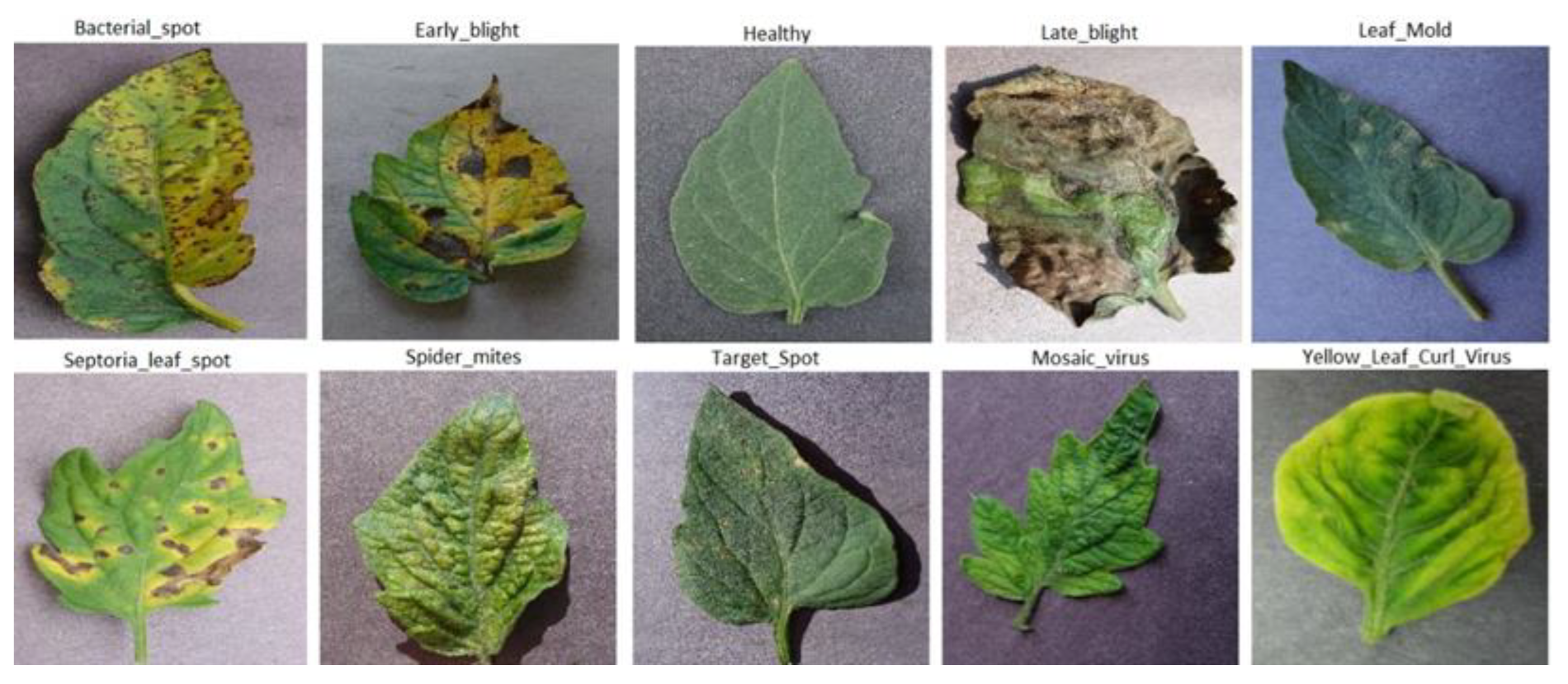
3.1. Dataset

In recent years, the scientific community has used the PlantVillage dataset [10] to propose solutions using artificial intelligence algorithms such as in [11,12,13,14,15,16,17,18,19,20,21]. This dataset is usually selected since it contains a wide variety of images corresponding to different diseases and crops. The tomato crop was chosen from this dataset because it is one of the most important vegetables in world agriculture, the second most important crop after the potato [22]. The size of the images is 256 × 256 px in RGB. Examples of the dataset can be seen in Figure 1.

Problems and challenges. PlantVillage contains images of tomato leaves taken in controlled environments, with at least nine different disease types and stages of development. It is one of the most referenced literature datasets for crop diseases. However, it has limitations that must be considered.

✓

Although the dataset preserves a certain homogeneity in the image capture conditions, such as the distance from the camera to the leaves, some classes were collected in different places. Moreover, in the original works [10,23], it is not indicated whether the tomato varieties are identical or different in each class. Therefore, there is uncertainty in this regard.

✓

Some morphological features of the leaves could be due to phenotypic and genotypic aspects of the variety and not necessarily a consequence of the disease. For example, in [24], the authors classified the silhouette of the leaves, obtaining an accuracy of 52.3% based on the ResNet-50 model.

✓

The dataset was made with images captured in different lighting and background conditions for each class, resulting in a classification bias. This was detected by the same authors in [24], who classified the backgrounds of the images, obtaining an accuracy of 62.3%. They recommend performing segmentation and eliminating the background before any classification procedure.

✓

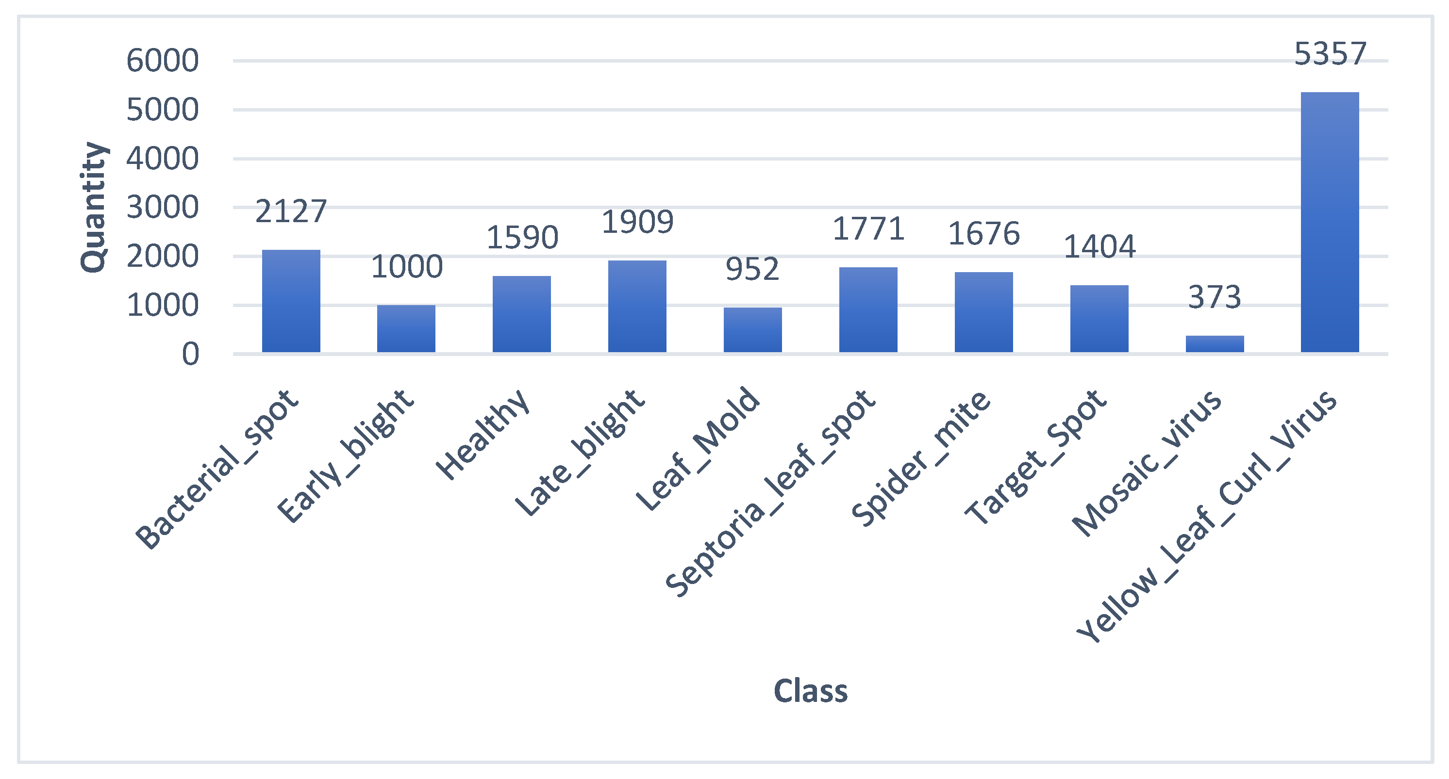
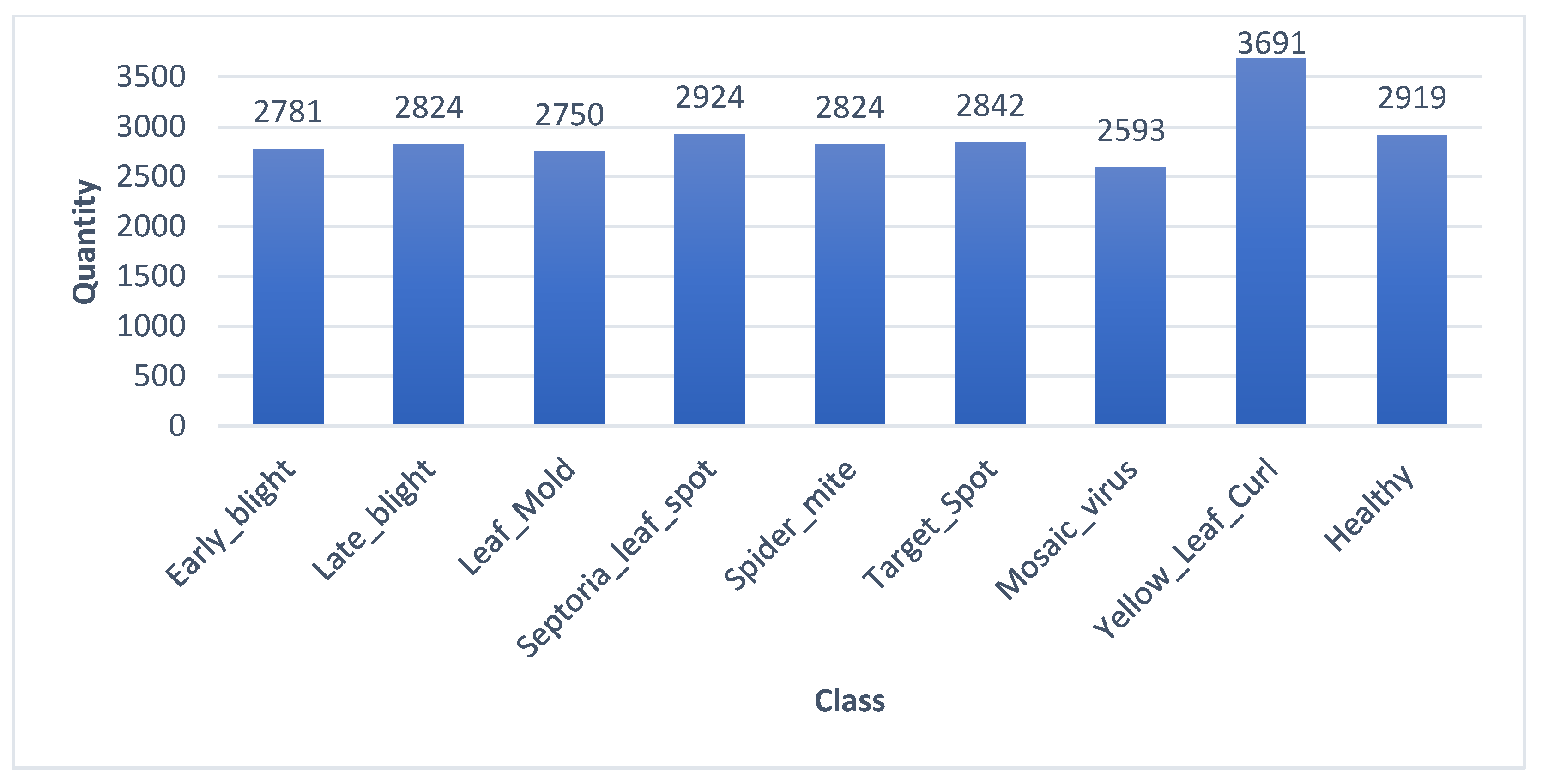
The dataset significantly differs in the number of images for some classes. An imbalance of the classes can be observed mainly between the mosaic virus class and the yellow leaf curl class, as seen in Figure 2.

3.2. Metrics

There are many ways to measure the performance of models used for classification in supervised learning. Nonetheless, metrics based on the confusion matrix were used in this research.

The confusion matrix is one of the most used tools in machine learning for evaluating classification models [25,26]. It is a matrix that compares the number of predictions for each class that are correct and those that are incorrect. The four main metrics that are extracted from the confusion matrix are:

• Accuracy (1): The overall accuracy of a model is simply the number of correct predictions divided by the total number of predictions. The model’s prediction accuracy is measured as a percentage value between 0 and 1, with a value of 1 indicating a perfectly performing model. Accuracy can be defined as the ratio of correct predictions to the total number of predictions.

$$Accuracy=\frac{TP+TN}{TP+TN+FP+FN}$$

(1)

• Precision (2): Measures how well the model correctly identifies the positive class. Using only this metric to optimize a model would minimize false positives.

$$Precision=\frac{TP}{TP+FP}$$

(2)

• Recall (3): Measures how good the model is at correctly predicting all positive observations in the dataset. However, it does not include information on false positives.

$$Recall=\frac{TP}{TP+FN}$$

(3)

• F1-score (4): The harmonic mean of Precision and Recall. The F1-score returns a number in a range between 0 and 1. If the value is 1, this indicates perfect Precision and Recall. If the value is 0, the Precision or Recall is 0. The higher the value of F1, it can be said that there is better the balance between the two metrics.

  $$F1=2\times \frac{Precision\times Recall}{Precision+Recall}$$

  (4)

  where:

• TP (True Positives): The number of positive observations the model correctly predicted as positive.
• FP (False Positive): The number of negative observations the model incorrectly predicted as positive.
• TN (True Negative): The number of negative observations the model correctly predicted as negative.
• FN (False Negative): The number of positive observations the model incorrectly predicted as negative.

3.3. Convolutional Neural Networks (CNNs) Selected for This Research

State-of-the-art small CNNs were used for disease classification based on their textural properties. The CNNs preselected for the experiments were MobileNet [27], MobileNetV2 [28], MobileNetV3 [29], EfficientNetB0 [30], NasNetMobile [31], SqueezeNet [32], and ShuffleNet [33].

The main characteristic for selecting the networks is their easy implementation in devices with low computational capacity, such as smartphones or Raspberry microcontrollers.

3.4. Method for Hyperparameter Optimization

For hyperparameter optimization, there are several techniques. We analyzed four of them:

• Grid Search [34].
• Randomized Grid Search [35].
• Bayesian Optimization [36].
• Genetic Algorithms [37].

The Grid Search and Randomized Grid Search techniques are simple to implement and are probably the most used by many researchers and engineers to optimize hyperparameters [38]. Nonetheless, these techniques have a “brute force” approach, which means that hyperparameter options are chosen based on intuition or experience and are tested, hoping that the “best” will be found among the chosen options.

Their advantage is that they are simple to implement and fast. However, these techniques are also known as “uninformed” because the search is performed without considering previously obtained results of hyperparameter combinations [39,40].

On the other hand, the “informed” methods follow an iterative sequential process where the best combinations of hyperparameters are sought, considering the results of previous searches based on some optimization algorithm. The most used methods of this type are Bayesian Optimization and Genetic Algorithms. A comparison of the different methods can be seen in [39].

The Grid Search and Randomized Grid Search methods were discarded for this work to rely on a more robust method. The method was selected between Bayesian and Genetic Algorithms optimization. A search was carried out in the literature in which the pros and cons of each are elucidated [38,39,40,41,42,43]. Based on the conclusions of these works, the following can be summarized:

• Optimization with Genetic Algorithms does not require any probabilistic model and works directly with the objective function. On the other hand, Bayesian Optimization uses a surrogate function, making it more efficient in using computational resources since it simplifies the original function, typically unknown in the case of neural networks.
• This means that fewer experiments are needed to achieve acceptable results. Furthermore, although in some studies, the results with Genetic Algorithms are better, the difference is insignificant.
• Genetic Algorithms have excellent parallelism capabilities, so the genetic algorithm performs very well when solutions are stored in memory, which can be improved over time. On the other hand, Bayesian Optimization cannot exploit parallelism because each experiment depends on the previous one. This makes optimization with Genetic Algorithms a more computationally demanding method.
• More characteristics differentiate them, but for this study, the requirement of less computational capacity by Bayesian Optimization makes it more suitable for selecting hyperparameters. Consequently, this was the method selected.

4. Results and Analysis

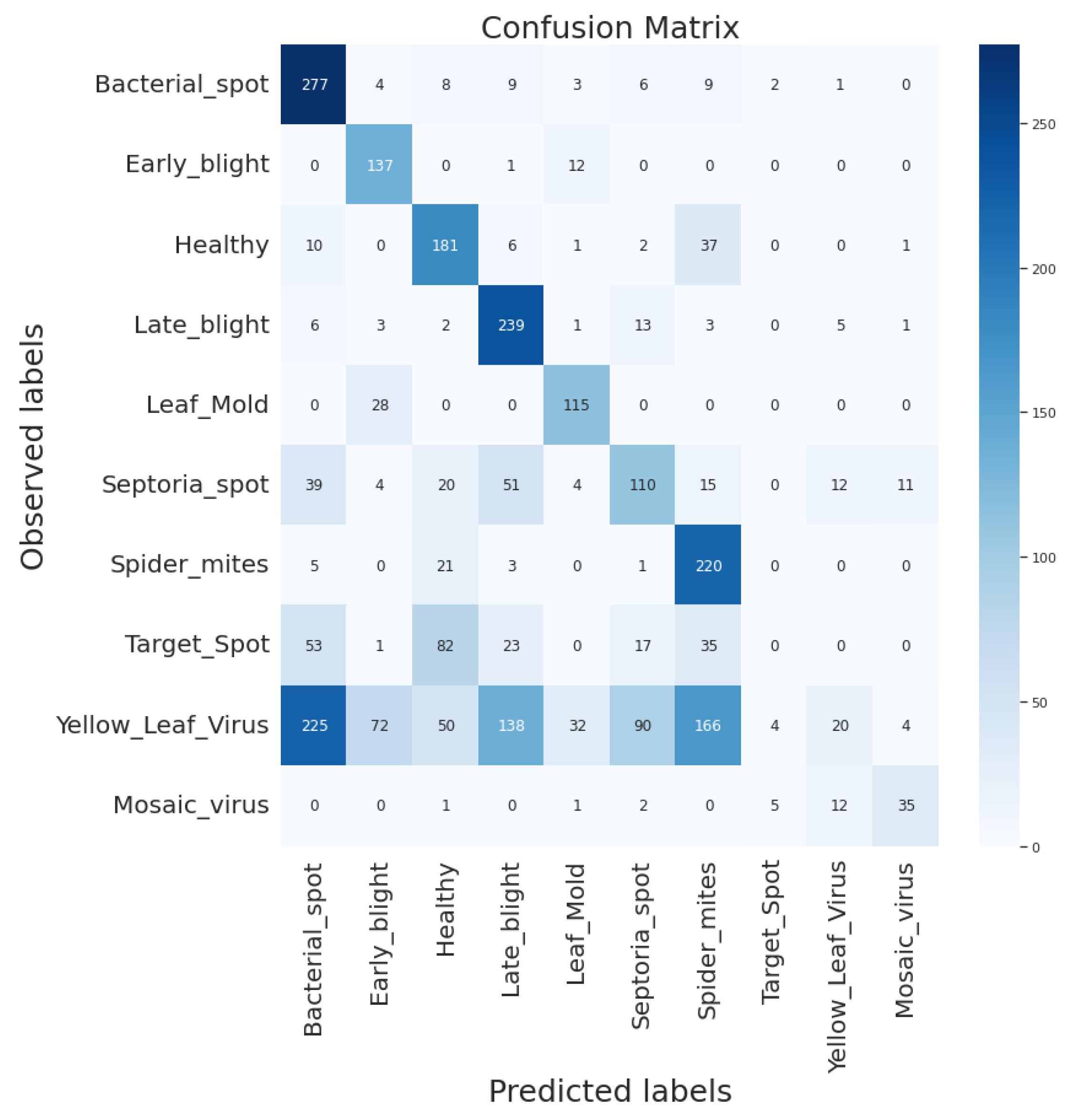
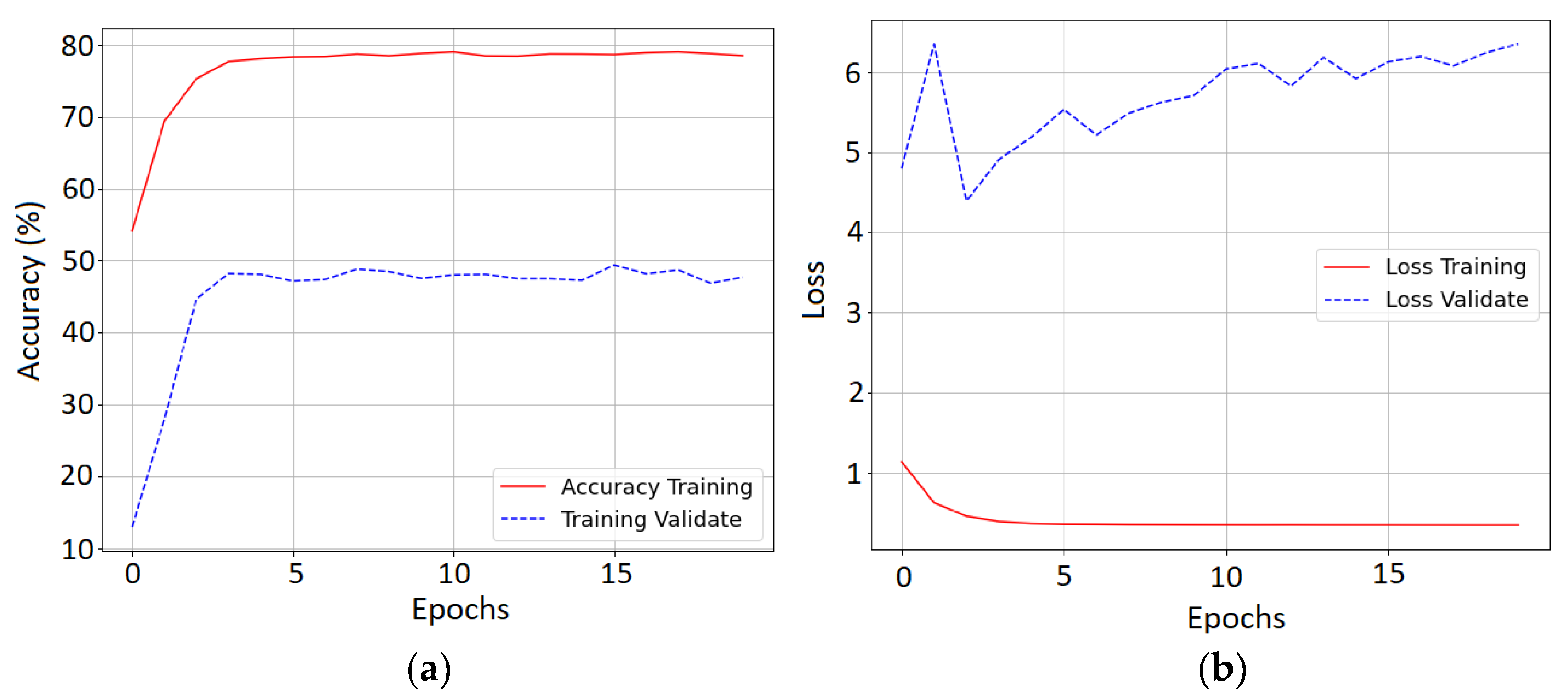
4.1. Effect of Leaf Shape on Disease Classification

The images in the dataset used in this research were biased due to the shape of the leaves. Although this bias is reported in the literature [24], a test was performed to measure its magnitude in this work.

✓

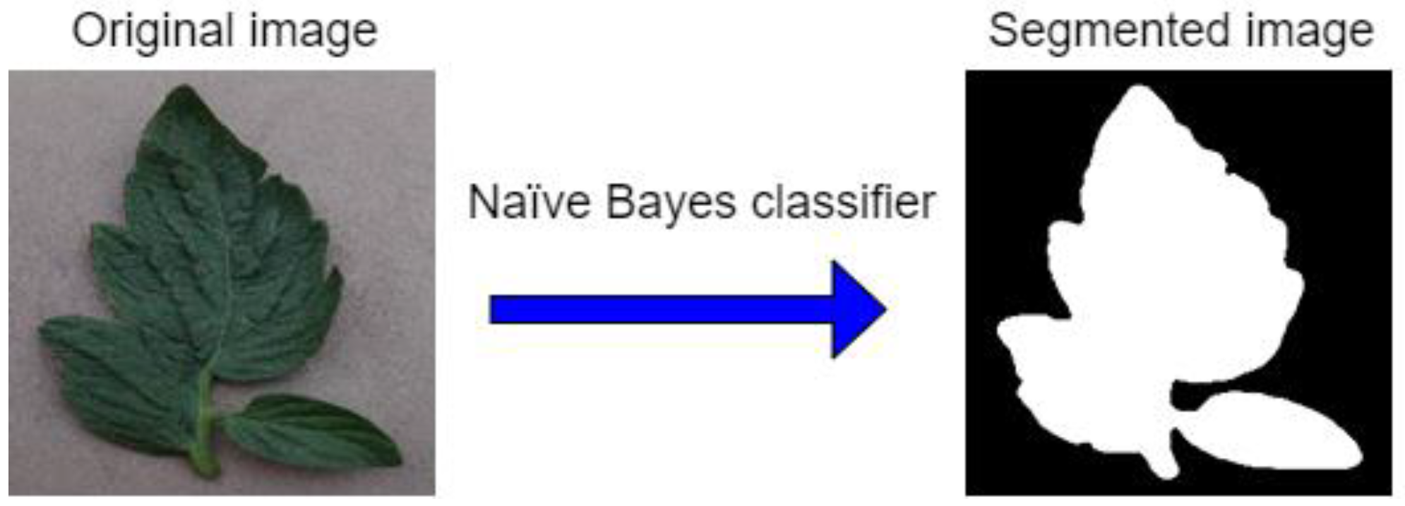
Binary segmentation was performed with Naïve Bayes classifier to obtain the silhouette of the leaves (Figure 3).

✓

Data augmentation was performed to eliminate the negative effect of data imbalance over the silhouette dataset.

✓

Training of the ResNet-50 model was carried out with the binary images, similar to [24].

✓

The hyperparameters used for model training were learning rate = 0.00234, optimizer = SGD (Stochastic Gradient Descent), epochs = 20, loss = categorical cross-entropy.

Figure 3. Example of the silhouette images (segmented image) used for training.

Figure 3. Example of the silhouette images (segmented image) used for training.

Figure 4 shows the confusion matrix results, in which a significant number of true positives (matrix diagonal) were correctly classified only considering the leaf’s shape. However, the model did not classify the Target spot class. Almost all samples of this class were classified in other classes. Hence, all their metrics are zero in

Table 1. Training results of the ResNet-50 model with the silhouettes dataset.

Class	Precision	Recall	F1-Score	Samples
Bacterial spot	0.4504	0.8683	0.5931	319
Early blight	0.5502	0.9133	0.6867	150
Healthy	0.4959	0.7605	0.6003	238
Late blight	0.5085	0.8755	0.6433	273
Leaf mold	0.6805	0.8042	0.7372	143
Septoria spot	0.4564	0.4135	0.4339	266
Spider mites	0.4536	0.8800	0.5986	250
Target spot	0.0000	0.0000	0.0000	211
Yellow leaf virus	0.4000	0.0250	0.0470	801
Mosaic virus	0.6731	0.6250	0.6481	56
Accuracy			0.4928	2707
Macro avg	0.4669	0.6165	0.4988	2707
Weighted avg	0.4334	0.4928	0.3898	2707

.

Figure 5 and Table 1 show the results of the training and prediction with the test dataset consisting of only the silhouette leaves. An accuracy of 49.28% is observed, close to the result reported in [24] of 52.3%. It can even be seen how for some classes, it has a considerably high Recall (proportion of instances belonging to the class correctly classified), for example, 91.33% in the early blight class, 88% for spider mites, and 87.55% in the late blight class. The findings confirm what is reported in the literature and ratify the importance of isolating the shape of the leaves to classify plant diseases.

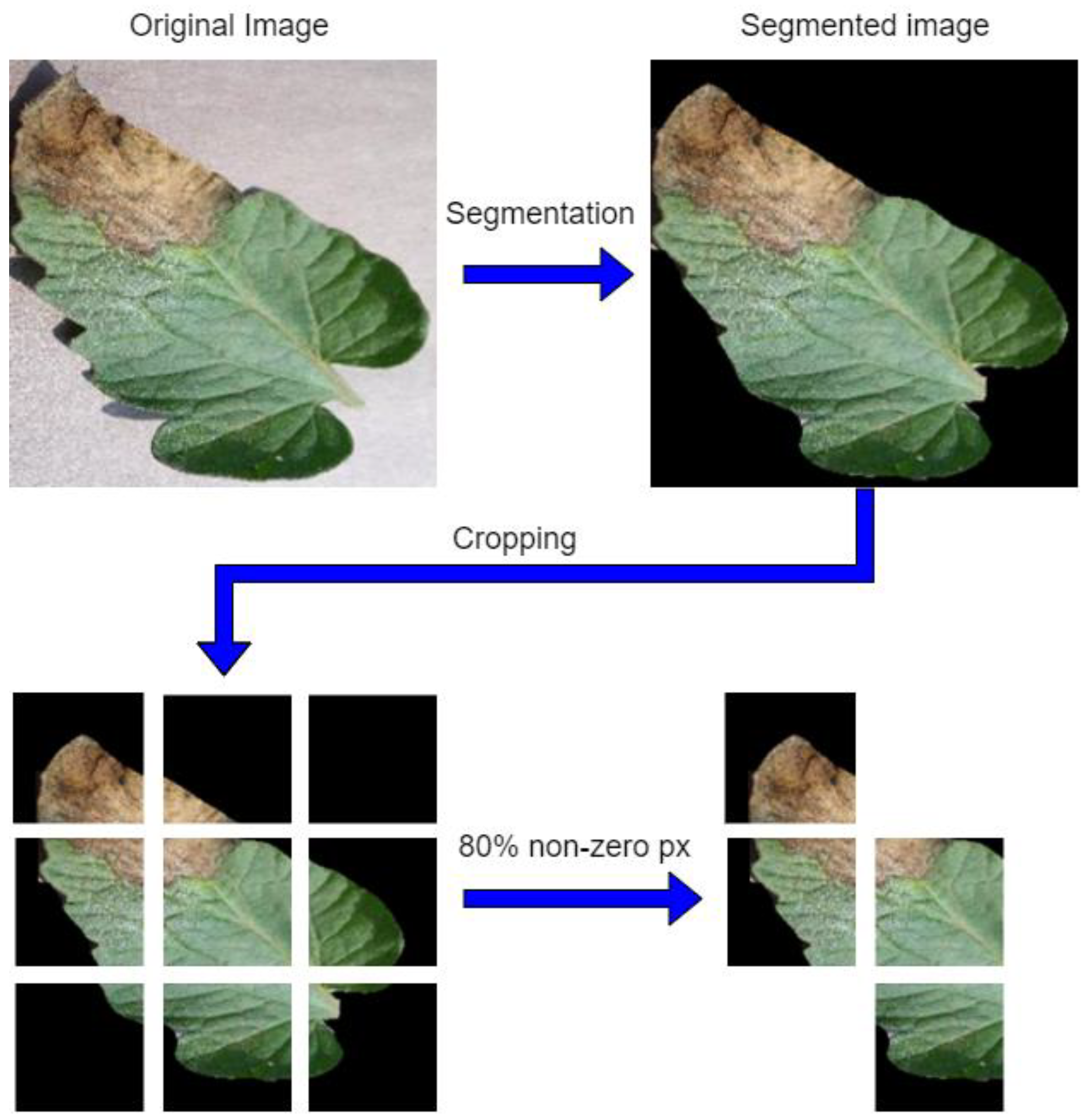
4.2. Plant Disease Detection Strategy Based on Image Texture

Image cropping. This research proposes cropping the original dataset images to isolate the morphological characteristics from the classification. The proposed process consists of the following steps:

(a)

The original images were segmented to remove background noise. This was performed with the segmentation method based on the machine learning Naive Bayes Algorithm.

(b)

The segmented image was subdivided into nine tiles of 85 × 85 × 3 pixels each, and only those with more than 80% of pixels corresponding to the object of interest (the leaves) were selected; the other tiles were eliminated (Figure 6).

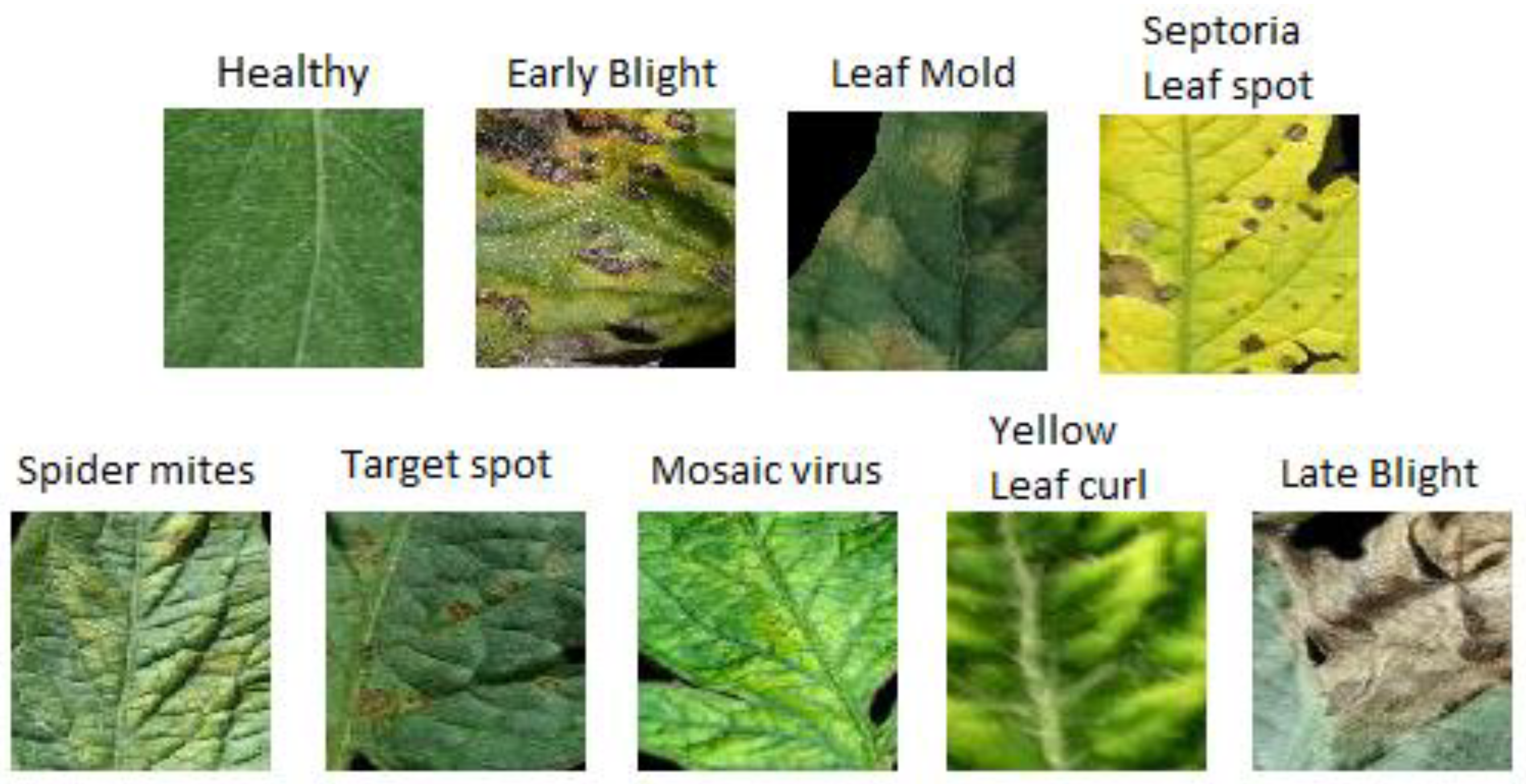
(c)

The selected tiles formed the dataset for training. Figure 7 shows an example of each class of the new dataset. The bacterial spot class was removed because it presents different stages of the disease in the original dataset, which represents an additional challenge since the early stages present significant similarities with the healthy class and do not allow its correct classification.

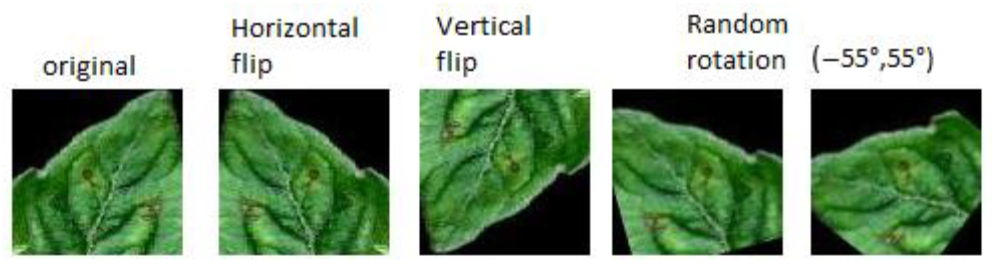
4.3. Data Balance

An imbalance of classes similar to the original dataset could be observed, so balancing was carried out by applying data augmentation for the first seven classes and reducing random data for the yellow leaf curl class, obtaining the results for a total of 26,148 images. The data augmentation techniques applied were horizontal flip, vertical flip, and random rotation (−55°, 55°) (Figure 8 and Figure 9).

The new dataset was divided into training, validation, and testing. Although there is no standard rule for this subdivision, it was realized following similar works in the literature, which show divisions generally between 70% and 80% of data for training and between 20% and 30% for validation and test data (

Table 2. Number of images in the new dataset. Training, validation, and test subsets.

Class	Train	Validation	Test	Total
Early_blight	2031	543	207	2781
Late_blight	2016	517	291	2824
Leaf_Mold	2088	531	131	2750
Septoria_leaf_spot	2014	561	349	2924
Spider_mite	2015	533	276	2824
Target_Spot	2084	540	218	2842
Mosaic_virus	2042	502	49	2593
Yellow_Leaf_Curl	2167	503	1021	3691
Healthy	2055	559	305	2919
Total	18,512	4789	2847	26,148
Percentage	71%	18%	11%	100%

).

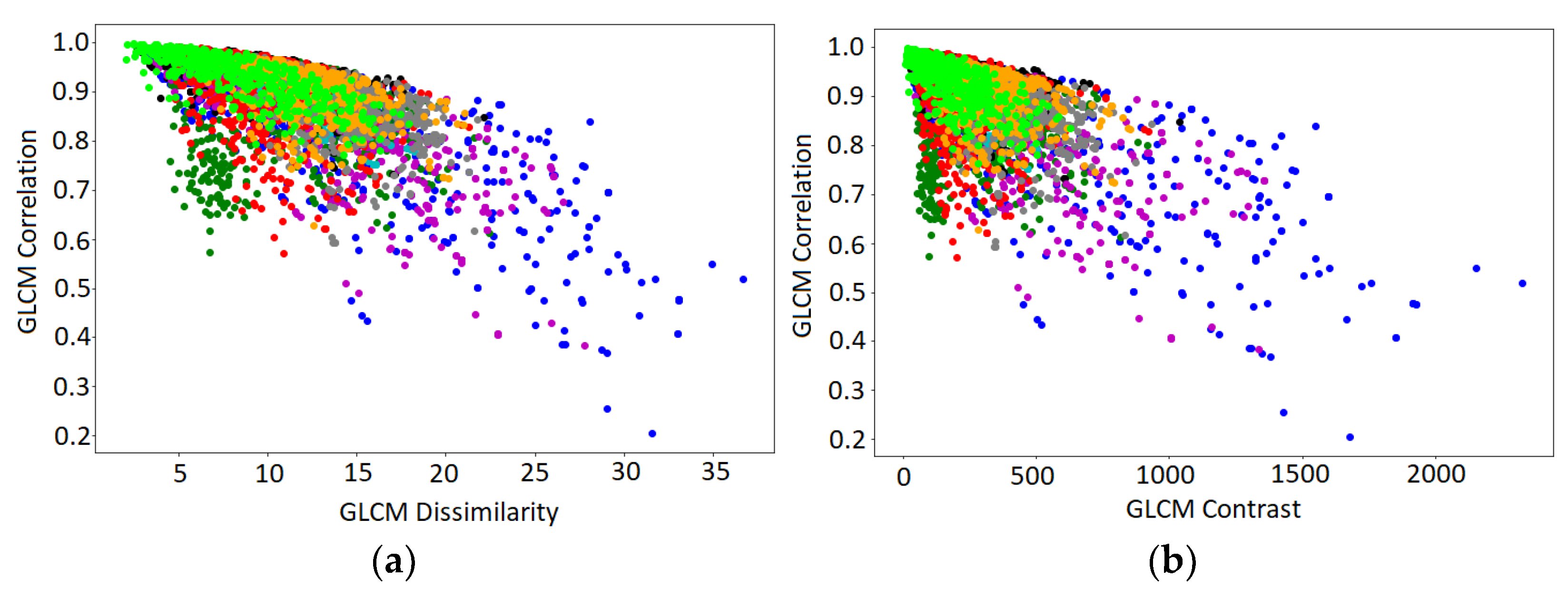
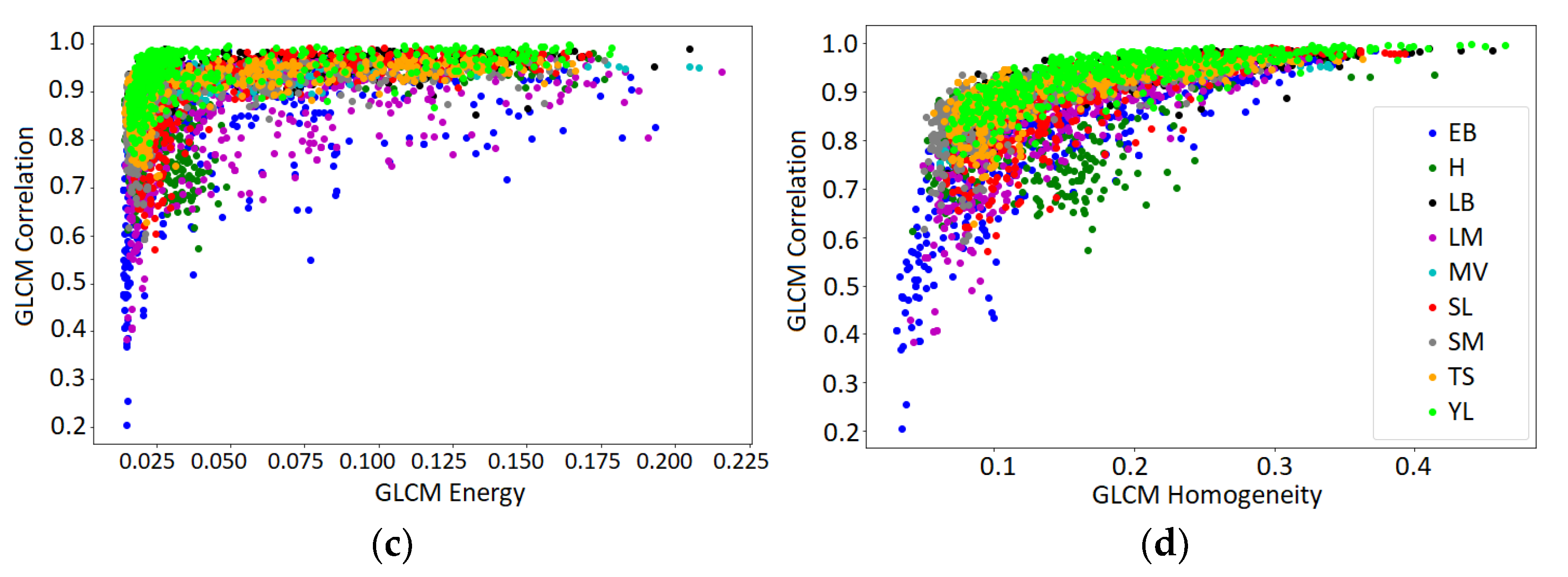
4.4. Predictive Power of Texture Features

In order to obtain a degree of interpretability for the classification methods to be used, we sought to know the predictive power of texture features in the case of diseases that affect plants. For this reason, the GLCM (Gray Level Co-occurrence Matrix) method was used to extract and explore the features with machine learning methods. GLCM is a statistical method for extracting texture features that consider the spatial relationship of pixels. This method constructed a gray-level co-occurrence matrix (GLCM), also known as a gray-level spatial dependence matrix [44].

The GLCM functions characterize an image’s texture by calculating how often pairs of pixels with specific values and spatial relationship occur in an image, creating a GLCM, and then extracting statistical measures from this matrix. The GLCM method functions do not provide information about the objects’ shape but rather about the spatial relationships of the pixels. The texture features extracted were Homogeneity, Contrast, Correlation, and Dissimilarity [45]

$$Contrast={{\displaystyle \sum }}_i {{\displaystyle \sum }}_j{\left(i-j\right)}^2{C}_{ij}$$

(5)

$$Correlation={{\displaystyle \sum }}_i {{\displaystyle \sum }}_j\frac{\left(i-{\mu }_i\right)\left(j-{\mu }_j\right)C_{ij}}{{\sigma }_i{\sigma }_j}$$

(6)

$$Homogeneity={{\displaystyle \sum }}_i {{\displaystyle \sum }}_j\frac{C_{ij}}{1+\left|i-j\right|}$$

(7)

$$Dissimilarity={{\displaystyle \sum }}_i {{\displaystyle \sum }}_j{C}_{ij}\left|i-j\right|$$

(8)

where:

• i = row number.
• j = column number.
• µ = mean of the GLCM (an estimate of all pixel intensities that contribute to the GLCM).
• σ = variance of the pixel intensities that contribute to the GLCM.
• C = element ij of the normalized GLCM.

Contrast measures the gray level variations between reference pixels and their neighbors (5). The correlation indicates the linear dependence of gray levels in the GLCM (6). Homogeneity is usually inversely related to contrast and indicates the similarity of off-diagonal elements in the GLCM (7). Finally, dissimilarity is a measure of the distance between pairs of pixels in the region of interest (8) [45].

The analysis was carried out with the skimage.feature library and its greycomatrix, greycoprops functions, with which the combination of distance and angle that best separated the groups was sought for two dimensions, pairwise combinations of the extracted features vs. the correlation. The results of this analysis are shown in Figure 10. There are groupings due to a high correlation between the elements of the same class. However, there is also a correlation between the classes, which represents a challenge of high complexity if you want to separate the classes based only on these combinations of characteristics.

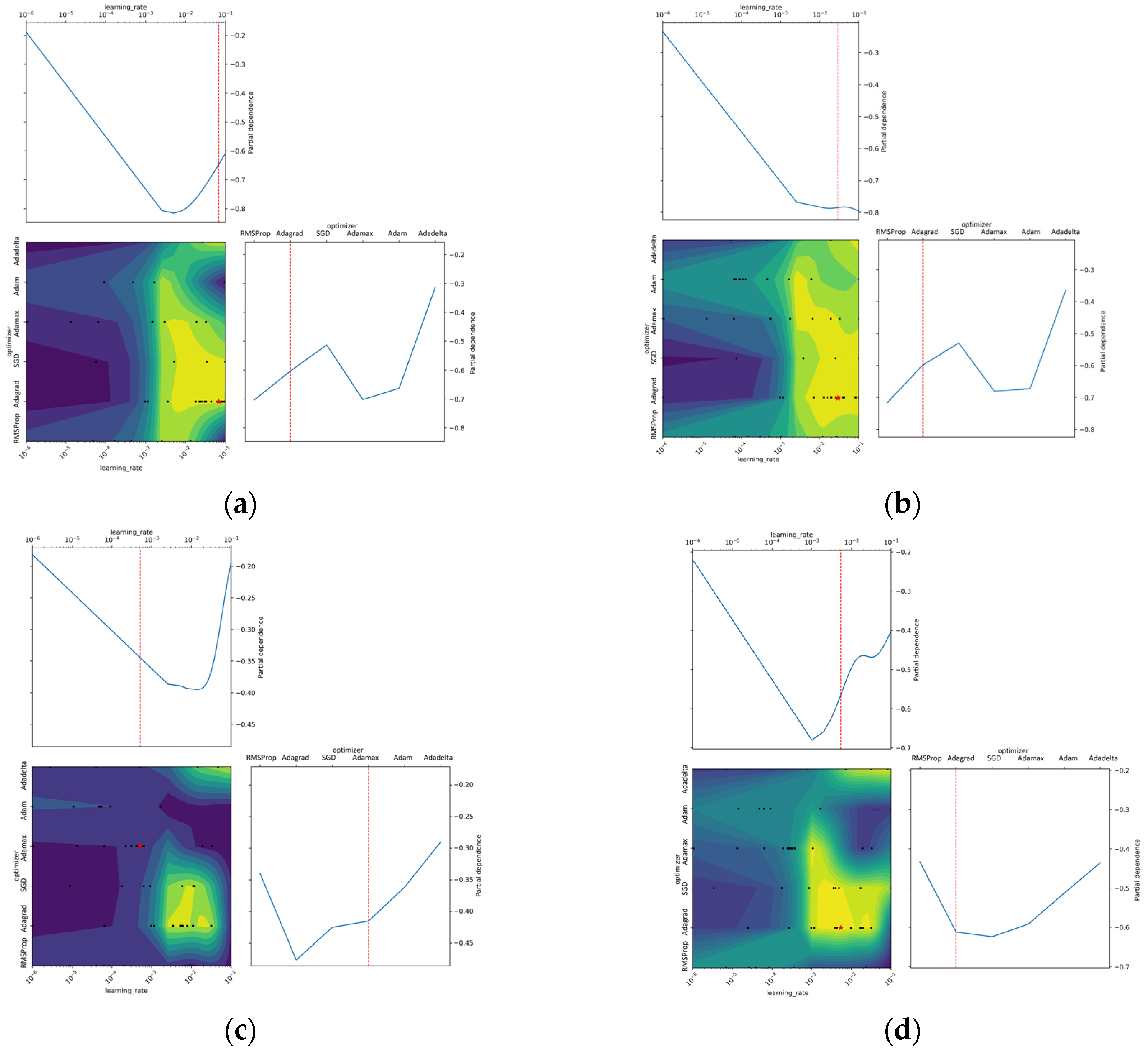
4.5. Hyperparameter Optimization

The Bayesian Optimization method was applied to the seven models chosen for this study, and the results can be seen in

Table 3. Results of the Bayesian Optimization applied to the preselected models.

Model	Optimizer	Learning Rate	Accuracy
MobileNet	Adagrad	0.06851166	0.9197443
MobileNetV2	Adagrad	0.00537715	0.9088542
SqueezeNet	Adagrad	0.02899546	0.8979640
NasNetMobile	Adamax	0.00051483	0.8411458
ShuffleNet	Adagrad	0.03231302	0.8671875
MobileNetV3	SGD	0.03170745	0.3214962
EfficientNetB0	Adamax	1.06 × 10−6	0.1387311

. The method was applied with the SKOPT library from scikit-optimize [46].

The optimization function and the learning rate were the two hyperparameters chosen for optimization. The optimization functions tested were RmsProp, Adagrad, SGD, Adamax, Adam, and Adadelta. The learning rate was defined in a range from 1 × 10⁻⁶ to 1 × 10⁻¹ for the search.

As can be seen in Table 3, the results of the MobileNetV3 and EfficientNetB0 networks did not converge. Their accuracy was below 33% for MobileNetV3 and less than 14% for EfficientNetB0. Thus, they were discarded for the phase of training with the hyperparameters found. Five epochs were used in each iteration for the optimization process, and a total of 100 iterations were extended for each optimization.

Partial dependence plots (PDP) constitute a model-agnostic interpretability method in machine learning [47]. In the plot, the vertical axis shows the average probability of the predictions, and the horizontal axis shows the values of the hyperparameters. The blue line captures how the average predicted probability changes as the hyperparameter values change. It is observed that the highest probability of the predictions occurs in the lower part of the curve. The calculation of PDP has a causal interpretation. By changing one of the hyperparameters, the changes in the predictions are measured [43,47]. Doing this analyzes the causal relationship between the hyperparameter and the prediction. Figure 11 shows the PDP produced by the Bayesian Optimization in this study. Again, the partial dependence shows the average effect on the predictions as the value of the hyperparameters changes, in this case, the optimizer and the learning rate.

4.6. Training Results

The five models with the best performance on Bayesian Optimization were chosen to be trained and compared. The training was carried out on the Google Colab platform with access to GPU. The NVIDIA brand GPU used has the following characteristics (Figure 12).

Training loss. Figure 13 shows the evolution of the loss during training. The employee loss function was categorical cross-entropy, also called log loss or logistic loss. With this function, each predicted class probability is compared to the desired output 0 or 1 of the actual class. Then, a loss is calculated that penalizes the probability based on how far it is from the expected value. The error penalty is logarithmic. The value is large for significant differences close to 1 and is small for minor differences that tend to be 0. The highest loss of approximately 0.6 was obtained for the NasNet model. SqueezeNet obtained the best performance, with a value close to 0.2.

Accuracy: As mentioned above, the overall accuracy of a model is simply the number of correct predictions divided by the total number of predictions resulting in a percentage value. This measurement is performed simultaneously with the data selected for training and validation. The main objective is that the two results do not diverge significantly. In the case of the training carried out with the selected models, the best accuracy with the validation data was obtained with the MobileNet model, close to 95%. On the other hand, the lowest accuracy was again obtained with the NasNet model. It is also important to highlight that both (loss and accuracy) behaviors show no overfitting since the gap between the training and validation results remains constant and is not significantly large (Figure 14).

4.7. Analysis

Although the metrics obtained from the confusion matrix and test data shown in Figure 15 and

Table 4. Metrics obtained from the confusion matrix (Macro Avg).

Model	Accuracy	Precision	Recall	F1-Score	Parameters	MB *
MobileNet	96.31%	95.55%	95.93%	95.72%	3,762,056	28.7
SqueezeNet	95.05%	93.98%	93.95%	93.91%	120,760	1.2
NasNetMobile	95.01%	92.73%	94.22%	93.29%	5,495,132	64.7
MobileNetV2	94.59%	92.35%	94.20%	93.17%	3,741,448	28.8
ShuffleNet	91.50%	89.36%	90.80%	89.93%	969,256	8.2

* MB: Megabytes.

are generally valuable for the analysis, the objective was focused on Precision and Recall. This is because these metrics are considered the most important when dealing with the detection of diseases that can significantly affect the economy of a vegetable producer if the detection is not executed reliably.

MobileNet: When the classifier indicates that the sample data represent a specific disease, this is correct on average 95.55% of the time (Precision). In addition, it detects 95.93% of the diseases present on average (Recall).

SqueezeNet: When the classifier indicates that the sample data represent a specific disease, this is correct on average 93.98% of the time (Precision). In addition, it detects 93.95% of the diseases present on average (Recall).

NasNetMobile: When the classifier indicates that the sample data represent a specific disease, this is correct on average 92.73% of the time (Precision). In addition, it detects 94.22% of the diseases present on average (Recall).

MobileNetV2: When the classifier indicates that the sample data represent a specific disease, this is correct on average 92.35% of the time (Precision). In addition, it detects 94.20% of the diseases present on average (Recall).

For plant diseases, there are two aspects of vital importance in decision making for their control:

i.

The loss of crops represents high costs. Consequently, action must be taken quickly to control the disease’s focus and not apply chemical agents to larger areas.

ii.

The correct detection of the disease is necessary so as not to apply the wrong control agents, which can cause an increase in the resistance of the disease to subsequent controls.

Therefore, Precision and Recall are metrics that provide the most reliability for decision making in this context. Even though a model with better accuracy is correct most of the time, they make a prediction. Hence, if their Recall is lower than others, they miss more diseases. Consequently, improving this metric is essential as long as a reasonable computational cost is maintained for the hardware used in the solution.

In this sense, the model that presented the best performance in all metrics was MobileNet. The results are shown in

Table 5. Training results for the MobileNet model.

Class	Precision	Recall	F1-Score	Samples
Early blight	0.9755	0.9614	0.9684	207
Healthy	0.9408	0.9902	0.9649	305
Late blight	0.9500	0.9141	0.9317	273
Leaf mold	0.9489	0.9924	0.9701	131
Septoria spot	0.9384	0.9599	0.9490	349
Spider mites	0.9526	0.9457	0.9491	250
Target spot	0.9209	0.9083	0.9145	218
Yellow leaf virus	0.9931	0.9824	0.9877	1021
Mosaic virus	0.9796	0.9796	0.9796	305
Accuracy			0.9631	2847
Macro avg	0.9555	0.9593	0.9572	2847
Weighted avg	0.9634	0.9631	0.9631	2847

.

5. Conclusions, Limitations, and Future Work

This work proposes a disease classification strategy based on the texture features of the images and hyperparameter optimization for the training of small CNNs with the Bayesian Optimization technique.

The proposed strategy is justified in that the shape of the leaves has a predictive power that can bias the result of the classification. Furthermore, although diseases can influence the shape of the leaves in plants, they can also be determined by phenotypic and genotypic characteristics that are unknown to the study dataset.

The results show that it is possible to carry out a classification with competitive results using small convolutional neural network models that do not require a large computing capacity to be implemented.

Bayesian Optimization is an important alternative in the search for ideal hyperparameters and can shorten the development time of future artificial intelligence models based on CNNs.

This research was conducted with only a part of the PlantVillage dataset, which corresponds to images of diseases that affect tomato crops. Consequently, the research on the other species of plants in the dataset, such as potato, pepper, or apple crops, which are important economically worldwide, was not within the scope of this study.

One of the main limitations of this work is that the results are not compared with those obtained in previous works. However, reference is made to research that has trained algorithms with the original dataset in Section 3.

In future works, tests should be conducted with different sizes of images, which allow for improving the resolution for a better classification based on the texture caused by the diseases in the plant leaves.

Research should also be conducted to improve performance based on the Precision and Recall metrics because these give greater reliability in the timely and accurate identification of possible plant diseases.

It is necessary to conduct more research on optimizing other CNN hyperparameters, such as the number of layers and filters, as well as on different implementation strategies of these models to know the performance in natural conditions with energy and computing capacity limitations.

References

1. FAO. New Standards to Curb the Global Spread of Plant Pests and Diseases. 2019. Available online: https://www.fao.org/news/story/en/item/1187738/icode/ (accessed on 26 June 2022).
2. Vishnoi, V.K.; Kumar, K.; Kumar, B. Plant disease detection using computational intelligence and image processing. J. Plant Dis. Prot. 2020, 128, 19–53. [Google Scholar] [CrossRef]
3. Shurtleff, M.C.; Pelczar, M.J.; Kelman, A.; Pelczar, R.M. Plant disease. In Plant Pathology; Encyclopedia Britannica: Chicago, IL, USA, 2020; Available online: https://www.britannica.com/science/plant-disease (accessed on 3 March 2022).
4. Balram, G.; Kumar, K.K. Smart farming: Disease detection in crops. Int. J. Eng. Technol. 2018, 7, 33–36. [Google Scholar] [CrossRef] [Green Version]
5. Nagaraju, M.; Chawla, P. Systematic review of deep learning techniques in plant disease detection. Int. J. Syst. Assur. Eng. Manag. 2020, 11, 547–560. [Google Scholar] [CrossRef]
6. Hlaing, C.S.; Zaw, S.M.M. Tomato Plant Diseases Classification Using Statistical Texture Feature and Color Feature. In Proceedings of the 2018 IEEE/ACIS 17th International Conference on Computer and Information Science (ICIS), Singapore, 6–8 June 2018; pp. 439–444. [Google Scholar] [CrossRef]
7. Ahmad, N.; Asif, H.M.S.; Saleem, G.; Younus, M.U.; Anwar, S.; Anjum, M.R. Leaf Image-Based Plant Disease Identification Using Color and Texture Features. Wirel. Pers. Commun. 2021, 121, 1139–1168. [Google Scholar] [CrossRef]
8. Anjna; Sood, M.; Singh, P.K. Hybrid System for Detection and Classification of Plant Disease Using Qualitative Texture Features Analysis. Procedia Comput. Sci. 2020, 167, 1056–1065. [Google Scholar] [CrossRef]
9. Hossain, E.; Hossain, F.; Rahaman, M. A Color and Texture Based Approach for the Detection and Classification of Plant Leaf Disease Using KNN Classifier. Available online: https://ieeexplore.ieee.org/stamp/stamp.jsp?arnumber=8679247&casa_token=5JO9r1u5jY0AAAAA:OJrFyWAj5u93OE_CTKS3rBwjh0vBLhk3FpYeHtDvAp_bY4cz4l67Fbu1cTCoLgDqKjnplV6DoyFS&tag=1 (accessed on 21 August 2022).
10. Hughes, D.P.; Salathé, M. An Open Access Repository of Images on Plant Health to Enable the Development of Mobile Disease Diagnostics. 2015. Available online: https://doi.org/10.48550/ARXIV.1511.08060 (accessed on 20 July 2021).
11. Hidayatuloh, A.; Nursalman, M.; Nugraha, E. Identification of Tomato Plant Diseases by Leaf Image Using Squeezenet Model. In Proceedings of the 2018 International Conference on Information Technology Systems and Innovation (ICITSI), Bandung, Indonesia, 22–26 October 2018. [Google Scholar]
12. Kaur, M.; Bhatia, R. Development of an improved tomato leaf disease detection and classification method. In Proceedings of the 2019 IEEE Conference on Information and Communication Technology, Baghdad, Iraq, 15–16 April 2019; pp. 1–5. [Google Scholar]
13. Agarwal, M.; Singh, A.; Arjaria, S.; Sinha, A.; Gupta, S. ToLeD: Tomato Leaf Disease Detection using Convolution Neural Network. Procedia Comput. Sci. 2020, 167, 293–301. [Google Scholar] [CrossRef]
14. Gunarathna, M.; Rathnayaka, R. Experimental Determination of CNN Hyper-Parameters for Tomato Disease Detection using Leaf Images. In Proceedings of the 2nd International Conference on Advancements in Computing, Malabe, Sri Lanka, 10–11 December 2020; pp. 464–469. [Google Scholar] [CrossRef]
15. Hong, H.; Lin, J.; Huang, F. Tomato disease detection and classification by deep learning. In Proceedings of the 2020 International Conference on Big Data, Artificial Intelligence and Internet of Things Engineering, Fuzhou, China, 12–14 June 2020; pp. 25–29. [Google Scholar]
16. Jiang, D.; Li, F.; Yang, Y.; Yu, S. A Tomato Leaf Diseases Classification Method Based on Deep Learning. In Proceedings of the 2020 Chinese Control And Decision Conference (CCDC), Hefei, China, 22–24 August 2020; pp. 1446–1450. [Google Scholar] [CrossRef]
17. Saleem, M.H.; Potgieter, J.; Arif, K.M. Plant Disease Classification: A Comparative Evaluation of Convolutional Neural Networks and Deep Learning Optimizers. Plants 2020, 9, 1319. [Google Scholar] [CrossRef] [PubMed]
18. Kibriya, H.; Rafique, R.; Ahmad, W.; Adnan, S. Tomato Leaf Disease Detection Using Convolution Neural Network. In Proceedings of the 18th International Bhurban Conference on Applied Sciences and Technologies, Islamabad, Pakistan, 12–16 January 2021; pp. 346–351. [Google Scholar] [CrossRef]
19. Peyal, H.I.; Shahriar, S.M.; Sultana, A.; Jahan, I.; Mondol, H. Detection of Tomato Leaf Diseases Using Transfer Learning Architectures: A Comparative Analysis. In Proceedings of the 2021 International Conference on Automation, Control and Mechatronics for Industry 4.0 (ACMI), Rajshahi, Bangladesh, 8–9 July 2021; pp. 1–6. [Google Scholar] [CrossRef]
20. Sujatha, R.; Chatterjee, J.M.; Jhanjhi, N.; Brohi, S.N. Performance of deep learning vs machine learning in plant leaf disease detection. Microprocess. Microsyst. 2020, 80, 103615. [Google Scholar] [CrossRef]
21. Younis, H.; Khan, M.Z.; Mukhtar, H. Robust Optimization of MobileNet for Plant Disease Classification with Fine Tuned Parameters. In Proceedings of the2021 International Conference on Artificial Intelligence, Suzhou, China, 15–17 October 2021; pp. 146–151. [Google Scholar] [CrossRef]
22. Panno, S.; Davino, S.; Caruso, A.G.; Bertacca, S.; Crnogorac, A.; Mandić, A.; Noris, E.; Matić, S. A Review of the Most Common and Economically Important Diseases That Undermine the Cultivation of Tomato Crop in the Mediterranean Basin. Agronomy 2021, 11, 2188. [Google Scholar] [CrossRef]
23. Mohanty, S.P.; Hughes, D.P.; Salathé, M. Using Deep Learning for Image-Based Plant Disease Detection. Front. Plant Sci. 2016, 7, 1419. [Google Scholar] [CrossRef] [PubMed] [Green Version]
24. Wspanialy, P.; Moussa, M. A detection and severity estimation system for generic diseases of tomato greenhouse plants. Comput. Electron. Agric. 2020, 178, 105701. [Google Scholar] [CrossRef]
25. Sokolova, M.; Lapalme, G. A systematic analysis of performance measures for classification tasks. Inf. Process. Manag. 2009, 45, 427–437. [Google Scholar] [CrossRef]
26. Tharwat, A. Classification assessment methods. Appl. Comput. Inform. 2018, 17, 168–192. [Google Scholar] [CrossRef]
27. Howard, A.G. Mobile Nets: Efficient Convolutional Neural Networks for Mobile Vision Applications. 2017. Available online: http://arxiv.org/abs/1704.04861 (accessed on 20 July 2021).
28. Sandler, M.; Howard, A.; Zhu, M.; Zhmoginov, A.; Chen, L. MobileNetV2: Inverted residuals and linear bottlenecks. In Proceedings of the IEEE/CVF Conference on Computer Vision and Pattern Recognition (CVPR), Salt Lake City, UT, USA, 18–23 June 2018; pp. 4510–4520. [Google Scholar] [CrossRef]
29. Howard, A.; Sandler, M.; Chen, B.; Wang, W.; Chen, L.-C.; Tan, M.; Chu, G.; Vasudevan, V.; Zhu, Y.; Pang, R.; et al. Searching for MobileNetV3. In Proceedings of the 2019 IEEE/CVF International Conference on Computer Vision (ICCV), Seoul, Korea, 27 October–2 November 2019; pp. 1314–1324. [Google Scholar] [CrossRef]
30. Tan, M.; Le, Q.v. EfficientNet: Rethinking model scaling for convolutional neural networks. In Proceedings of the 36th International Conference on Machine Learning, Long Beach, CA, USA, 9–15 June 2019; pp. 10691–10700. [Google Scholar]
31. Tan, M.; Chen, B.; Pang, R.; Vasudevan, V.; Sandler, M.; Howard, A.; Le, Q.V. MnasNet: Platform-Aware Neural Architecture Search for Mobile. In Proceedings of the IEEE Computer Society Conference on Computer Vision and Pattern Recognition, Long Beach, CA, USA, 15–20 June 2019. [Google Scholar]
32. Iandola, F.N.; Han, S.; Moskewicz, M.W.; Ashraf, K.; Dally, W.J.; Keutzer, K. SqueezeNet: AlexNet-Level Accuracy with 50x Fewer Parameters and <0.5MB Model Size. 2016. Available online: http://arxiv.org/abs/1602.07360 (accessed on 20 July 2021).
33. Zhang, X.; Zhou, X.; Lin, M.; Sun, J. ShuffleNet: An Extremely Efficient Convolutional Neural Network for Mobile Devices. In Proceedings of the IEEE Computer Society Conference on Computer Vision and Pattern Recognition, Honolulu, HI, USA, 21–26 July 2017. [Google Scholar]
34. Jiménez, B.; Lázaro, J.L.; Dorronsoro, J.R. Finding optimal model parameters by deterministic and annealed focused grid search. Neurocomputing 2009, 72, 2824–2832. [Google Scholar] [CrossRef]
35. Bergstra, J.; Bengio, Y. Random Search for Hyper-Parameter Optimization Yoshua Bengio. 2012. Available online: http://scikit-learn.sourceforge.net (accessed on 20 July 2021).
36. Wu, J.; Chen, X.-Y.; Zhang, H.; Xiong, L.-D.; Lei, H.; Deng, S.-H. Hyperparameter optimization for machine learning models based on Bayesian optimization b. J. Electron. Sci. 2019, 17, 26–40. [Google Scholar] [CrossRef]
37. Aszemi, N.M.; Dominic, P. Hyperparameter Optimization in Convolutional Neural Network using Genetic Algorithms. Int. J. Adv. Comput. Sci. Appl. 2019, 10, 269–278. Available online: www.ijacsa.thesai.org (accessed on 10 August 2021). [CrossRef] [Green Version]
38. Liashchynskyi, P.; Liashchynskyi, P. Grid Search, Random Search, Genetic Algorithm: A Big Comparison for NAS. 2017. Available online: http://arxiv.org/abs/1912.06059 (accessed on 8 July 2022).
39. Alibrahim, H.; Ludwig, S.A. Hyperparameter Optimization: Comparing Genetic Algorithm against Grid Search and Bayesian Optimization. In Proceedings of the 2021 IEEE Congress on Evolutionary Computation (CEC), 28 June–1 July 2021; pp. 1551–1559. [Google Scholar] [CrossRef]
40. González, J. Still Optimizing in the Dark? Bayesian Optimization for Model Configuration and Experimental Design. University of Sheffield, Sheffield, UK. 2016. Available online: http://javiergonzalezh.github.io/presentations/talk_groningen2016.pdf (accessed on 10 August 2022).
41. Bochinski, E.; Senst, T.; Sikora, T. Hyper-parameter optimization for convolutional neural network committees based on evolutionary algorithms. In Proceedings of the 2017 IEEE International Conference on Image Processing (ICIP), Beijing, China, 17–20 September 2017; pp. 3924–3928. [Google Scholar] [CrossRef] [Green Version]
42. Tani, L.; Rand, D.; Veelken, C.; Kadastik, M. Evolutionary algorithms for hyperparameter optimization in machine learning for application in high energy physics. Eur. Phys. J. C 2021, 81, 170. [Google Scholar] [CrossRef]
43. Moosbauer, J.; Herbinger, J.; Casalicchio, G.; Lindauer, M.; Bischl, B. Explaining Hyperparameter Optimization via Partial Dependence Plots. Adv. Neural. Inf. Process Syst. 2021, 3, 2280–2291. [Google Scholar]
44. Raheja, J.L.; Kumar, S.; Chaudhary, A. Fabric defect detection based on GLCM and Gabor filter: A comparison. Optik 2013, 124, 6469–6474. [Google Scholar] [CrossRef]
45. Liu, X.; Aldrich, C. Deep Learning Approaches to Image Texture Analysis in Material Processing. Metals 2022, 12, 355. [Google Scholar] [CrossRef]
46. Louppe, G.; Head, T.; Kumar, M.; Nahrstaedt, H.; Shcherbatyi, L. Scikit-Optimize. Available online: https://github.com/scikit-optimize (accessed on 5 June 2022).
47. Molnar, C. Interpretable Machine Learning A Guide for Making Black Box Models Explainable. 2019. Available online: http://leanpub.com/interpretable-machine-learning (accessed on 10 August 2022).
Figure 1. Examples of original PlantVillage dataset [10].
Agriculture 12 01964 g001
Figure 2. Number of images in the original dataset for each class [10].
Agriculture 12 01964 g002
Figure 4. Confusion matrix results for the leaves’ silhouette classification with the ResNet50 model. Numbers in the matrix mean the samples classified in each class, and the colors help to identify where more samples are classified (darker colors).
Agriculture 12 01964 g004
Figure 5. Training record of the ResNet-50 model. (a) Training accuracy, (b) Training loss.
Agriculture 12 01964 g005
Figure 6. Example of cropping segmented images and selected tiles with more than 80% non-zero px.
Agriculture 12 01964 g006
Figure 7. Example of new dataset tiles by class.
Agriculture 12 01964 g007
Figure 8. Example of data augmentation on the new training dataset.
Agriculture 12 01964 g008
Figure 9. Number of resulting images after class balancing.
Agriculture 12 01964 g009
Figure 10. Graphical analysis of texture features extracted with GLMC. Correlation vs. (a) Dissimilarity, (b) Contrast, (c) Energy, (d) Homogeneity. EB: Early Blight, H: Healthy, LB: Late Blight, LM: Leaf Mold, MV: Mosaic Virus, SL: Septoria Leaf, SM: Spider Mite, TS: Target Spot, YL: Yellow Leaf.
Agriculture 12 01964 g010aAgriculture 12 01964 g010b
Figure 11. Partial dependence plots obtained for each combination of hyperparameters, with Bayesian Optimization applied to the selected CNNs. Red points and lines are the best hyperparameter combination for each model. (a) MobileNet, (b) SqueezeNet, (c) NasNetMobile, and (d) MobileNetV2.
Agriculture 12 01964 g011
Figure 12. GPU technical specifications from Google Colab.
Agriculture 12 01964 g012
Figure 13. Training results for loss of the four best-performing models: (a) MobileNet, (b) SqueezeNet, (c) NasNetMobile, and (d) MobileNetV2.
Agriculture 12 01964 g013
Figure 14. Training results for accuracy of the four best-performing models: (a) MobileNet, (b) SqueezeNet, (c) NasNetMobile, and (d) MobileNetV2.
Agriculture 12 01964 g014
Figure 15. Confusion matrix results of the four best-performing models: (a) MobileNet, (b) SqueezeNet, (c) NasNetMobile, and (d) MobileNetV2. Numbers in the matrix mean the samples classified in each class, and the colors help to identify where more samples are classified (darker colors).
Agriculture 12 01964 g015