Article

Addressing Rural–Urban Income Gap in China through Farmers’ Education and Agricultural Productivity Growth via Mediation and Interaction Effects

1
School of Economics, Shandong University of Finance and Economics, Jinan 250014, China
2
Faculty of Economics, Nankai University, Tianjin 300071, China
3
School of Agriculture, Policy and Development (SAPD), University of Reading, Reading RG6 6UR, UK
4
Faculty of Economics, Chiang Mai University, Chiang Mai 50200, Thailand
*
Author to whom correspondence should be addressed.
Agriculture 2022, 12(11), 1920; https://doi.org/10.3390/agriculture12111920
Submission received: 28 September 2022 / Revised: 26 October 2022 / Accepted: 10 November 2022 / Published: 15 November 2022

Abstract

:
Narrowing the rural–urban income gap is an important challenge in achieving sustained and stable economic and social development in China. The present study investigates the role of farmers’ education and agricultural productivity growth in influencing the rural–urban income gap by applying mediation, interaction, and quantile regression models to provincial panel data of China from 2003 to 2017. Results show that, first of all, China’s agricultural productivity (TFP) continues to improve, and it is mainly driven by technical change (TC), with no significant role of technical efficiency change (TEC) or stable scale change (SC). Improving farmers’ education not only directly narrows the rural–urban income gap but also indirectly improves agricultural productivity to further narrow the rural–urban income gap. Due to differences in income sources of farmers, the corresponding impacts of farmers’ education and agricultural productivity growth on the rural–urban income gap also differ. Policy recommendations include continued investments in farmers’ education and training as well as modernization of agricultural for higher productivity growth.

1. Introduction

The rural–urban income gap is an important problem in macroeconomic research [1]. The excessive rural–urban income gap has caused a series of problems, such as inefficient economic development and difficulty in comprehensive development [2]. According to the official definition of household income (defined by the National Bureau of Statistics, NBS), the rural–urban income ratio in China went up from 2.47 in 1997 to 3.14 in 2007, and it was 2.65 in 2019. Although the rural–urban income gap has eased in recent years, China’s rural–urban dual structure is still significant, and the income gap is still large, according to international standards [3,4,5]. How to reduce the rural–urban income gap and promote the coordinated development of urban and rural areas is one of the major challenges facing China [6]. In order to solve this problem and coordinate urban and rural development, the Chinese government has actively adopted a series of policies and measures, such as developing rural education and improving agricultural productivity, to increase farmers’ income and narrow the rural–urban income gap [7,8]. Increases in both education level and agricultural productivity can improve the urban–rural income gap, and there is a link between them. On the one hand, the development of education is conducive to improving the knowledge structure of farmers, facilitating farmers to engage in higher-income-generating activities and directly narrowing the income gap [9]. On the other hand, the development of education can help farmers to learn to use advanced production technology, thus promoting improvement of agricultural total factor productivity (TFP) [10]. The growth of TFP means increasing production and income, which indirectly reduces the urban–rural income gap to some extent.
Judging from the development experience of developed countries, the transition from an agricultural society to an industrial society is the only way for developing countries to develop their economies. During the period of social transformation, the rural–urban income gap will inevitably increase [11]. Therefore, the rural–urban gap is inevitable in any country and any social system. From the perspective of the impact of rural–urban income gap on social development, a reasonable income gap has a positive effect on economic development and social stability, while an unreasonable gap will have a negative effect on sustainable economic development [12]. To a certain extent, a reasonable rural–urban income gap can attract some rural residents to gather in cities, accept advanced ideas and production technology in cities under certain conditions, improve comprehensive quality, and have a positive effect on economic development and social stability. However, due to the large rural–urban income gap in China, the negative effect of income gap is dominant. An excessive rural–urban income gap will lead to the “middle income trap” in social and economic development, which will bring a series of consequences to economic and social development and lead to serious social problems. The rural–urban income gap will lead to lower purchasing power for rural residents, which has a certain inhibitory effect on farmers’ happiness and welfare [13]. At the same time, too large an income gap will make it difficult to activate the vast rural consumer market, reduce farmers’ marginal propensity to consume, and then influence investment multipliers, leading the country to fall into the “middle income trap”, thereby adversely affecting overall economic development [12].
To sum up, how to narrow the urban–rural income gap and rationally control the gap in China is an important issue. Narrowing the urban–rural income gap is beneficial in avoiding the “middle income trap”, expanding the rural consumer market, and ensuring the healthy and sustainable development of the Chinese economy. Therefore, the main purpose of this paper is to explore effective ways to narrow the urban–rural income gap through education and agricultural total factor productivity growth.
The structure of the paper is as follows: Section 2 summarizes the materials and methods that examines the urban–rural income gap and its influencing factors and the roles of education and agricultural total factor productivity, and the stochastic frontier model (SFM) and the dynamic panel model etc. Section 3 presents the empirical results. Finally, Section 4 discusses conclusions and policy implications and also summarizes the shortcomings of this research.

2. Materials and Methods

2.1. The Urban–Rural Income Gap and its Influencing Factors

The problem of the widening rural–urban income gap has aroused widespread concern among scholars and policymakers. Many studies start with an estimation of the rural–urban income gap. Wang et al. [14] found that China’s rural–urban income gap presents an “inverted U” shape. Song and Ma [15] used the Human Development Index to calculate the rural–urban income gap in China from 1990 to 2002 and found that during this period, the income gap continued to increase. Scholars generally believe that the rural–urban income gap has widened with China’s economic development [16]. Li and Luo [17] estimated the level of disguised subsidies received by urban and rural residents and further included such disguised subsidies into the estimation of the rural–urban income gap. Ji et al. [18] showed that China’s urban–rural income gap is very wide. If the difference of welfare between urban and rural residents is taken into account, the urban–rural income gap will be even wider. Although the urban–rural income gap has been narrowed, it still hovers at a high level [19].
Other studies focus on the factors influencing rural–urban income gap. Based on China’s export data and income survey data, Zhu et al. [20] found that upgrading the structure of export products helps reduce income inequality in China. Chen et al. [21] studied the relationship between urbanization and rural–urban income disparities in 31 provinces in China from 1978 to 2019 and concluded that there is a two-way causal relationship between urbanization and the rural–urban income gap. Weng et al. [22] studied the impact of rural transportation infrastructure investment on the income gap among residents and tested the impact of rural road supply on the income gap among farmers, using panel data from 30 provinces in China from 1993 to 2013. The study found that China’s rural roads have a “U-shaped” effect on the income gap among inter-provincial farmers. Wang et al. [23] found that the increase of government fiscal expenditure promoted widening of the rural–urban income gap. Wang et al. [4] believed that an increase in the proportion of non-agricultural industries would widen the rural–urban income gap because non-agricultural industries require higher-skilled labor. Although scholars have studied many influencing factors of the rural–urban income gap, most such studies are based on partial influencing factors. Therefore, in order to provide a comprehensive analysis of all possible factors, we choose indicators from seven aspects, including economic development, financial development, and so on, in order to construct an indicator system to study their influence on narrowing the rural–urban income gap.

2.2. The Influence of Education Level on the Rural–Urban Income Gap

According to the existing research, reasons for the gradual increase the in rural–urban income gap include many aspects, such as finance and the economy, at the present stage [24]. Among them, the unequal allocation of urban and rural educational resources is one of the important reasons, and rural areas are often in a disadvantageous position with regard to resource allocation [8,25]. Education has a certain productive function, which can effectively promote individuals to improve labor efficiency and enable workers to engage in jobs with higher wages. For farmers, it is one of the ways to increase their non-agricultural income and plays an extremely important role in narrowing the income gap [7,15]. Thus, education level is not only an important factor in determining income distribution but also an effective way to reduce the rural–urban income gap [2,26].
Anlimachie and Avoada [27] studied the impact of pre-tertiary education in Ghana on the rural–urban income gap using a sample survey of 120 teachers from 30 schools in a rural school district. Weng et al. [22] found that laborers with higher education levels are more likely to engage in non-agricultural jobs with higher wages, thereby widening the rural–urban income gap. This is consistent with the conclusions of Yuan et al. [24]. Chu and Hoang [2] found that the improvement of the education level can reduce the rural–urban income gap effectively. Through existing research, it can be found that improving the cultural level of farmers is of great significance to increasing farmers’ income, narrowing the rural–urban income gap and coordinating urban and rural development [28,29]. Therefore, referring to the research of Gao et al. [29], we select the illiteracy rate of farmers as the variable to measure the education level of farmers, and we analyze the impact of the education level of farmers on the rural–urban income gap.

2.3. The Influence of Agricultural TFP on the Rural–Urban Income Gap

As China is a big agricultural country, agriculture is the basic industry on which China depends for its survival. On one hand, agriculture plays an important role in supporting other sectors of the national economy [30]. On the other hand, the development of agricultural production is directly related to the improvement of farmers’ income level and living standards [31]. The Chinese government has always attached great importance to agricultural production and development, and it has continued to increase agricultural investment. The Chinese government’s research funding for agriculture has been growing at an annual rate of more than 20% (NSBC). The Chinese government has continued to promote the modernization of agriculture and rural areas and implemented a rural revitalization strategy, resulting in a notable increase in agricultural TFP [23]. Improving agricultural TFP is a necessary condition for realizing agricultural modernization and sustainable development and also an indispensable part of China’s modernization [32]. Meanwhile, the increase in agricultural productivity provides opportunities for agricultural labor to transfer from agriculture to other, non-agricultural sectors, increasing farmers’ non-agricultural income and narrowing the rural–urban income gap [30]. Wang et al. [33] believed that improvement of agricultural productivity effectively promoted the transfer of labor force from agriculture to non-agricultural industries, increased farmers’ income, narrowed the income gap between urban and rural areas, and thus promoted economic growth. Li et al. [34] measured the TFP of the agricultural environment, using agricultural production data of 30 provinces in China from 2001 to 2017, and then studied its impact on the rural–urban income gap. The results show that the growth of the TFP of the agricultural environment further widens the rural–urban income gap. Hu et al. [32] believe that increasing agricultural TFP can reduce the rural–urban income gap by increasing farmers’ income. Therefore, at this stage, given contrasting conclusions in the literature, it is necessary to study whether and what kind of impact China’s agricultural TFP has on the rural–urban income gap.
It can be seen that the rural–urban income gap is one of the important factors affecting the living standards of residents and the sustainable and stable development of society. Governments have taken active measures to curb widening rural–urban income gaps. Therefore, accurately grasping the current situation of the rural–urban income gap and its influencing factors is an important prerequisite for alleviating the excessive rural–urban income gap. Existing studies have conducted extensive and in-depth research on the rural–urban income gap and its influencing factors in China in recent years. However, there are only a few studies on the impact of agricultural TFP and farmers’ education level on the rural–urban income gap, and studies on their interaction effects in narrowing the rural–urban income gap need to be further deepened. Therefore, it is of both theoretical and practical significance to select appropriate econometric methods to study the joint role of agricultural TFP and farmers’ education level in narrowing the rural–urban income gap in China. In addition, as the largest developing country in the world, in the context of China, analyzing the rural–urban income gap may provide a reference for other developing countries to narrow their income gaps [35].
With reference to existing research, there is a question of whether there is an indirect way to improve the education level of farmers and the reduce rural–urban income gap while concurrently increasing agricultural TFP. At present, there is no relevant research in academia regarding this question, but it can be analyzed through two links. First, the improvement of farmers’ education level can improve agricultural TFP significantly. Using data from three Brazilian agricultural censuses, Rada et al. [36] found that education significantly improves agricultural productivity. Liu et al. [37] believed that the illiteracy rate of farmers had a significant negative impact on agricultural TFP. Second, the improvement of agricultural TFP can narrow the rural–urban income gap. If all the above links are true, then there is an indirect way for farmers’ education level to affect the rural–urban income gap through agricultural TFP. Therefore, in this research we examined the mediating effect pathway as well.
Many regression models have been applied to analyze the influencing factors of the urban–rural income gap, among which dynamic panel data is one of the cutting-edge models. For example, Wang et al. [5] used dynamic panel data models to investigate how urban-biased land development policy impacts the urban–rural income gap in China. Zhang and Hu [38] investigated the impact of the urban–rural income gap on fertilizer use intensity using a dynamic panel data analysis. Huang and Zhang [39] found that financial inclusion narrows urban–rural income inequality in the long run using a dynamic panel fixed-effect approach. In addition, mediation effects and interaction effects are often measured in panel data models, e.g., Yuan et al. [40] and Liu et al. [14]. Before analyzing the impact of agricultural TFP on the urban–rural income gap, we need to measure the agricultural TFP. The main methods used in the current literature are data envelope analysis (DEA) and stochastic frontier analysis (SFA). In contrast to DEA methods, the production frontier of each individual is random, which may be more in line with the actual agricultural production processes of individual farmers. Furthermore, most of the studies used SFM to analyze agricultural productivity [41,42,43]. Therefore, we decided to measure the agricultural TFP by SFM and analyze the impact of farmers’ education and agricultural TFP on the urban–rural income gap with the help of dynamic panels.
Given this backdrop, the specific objectives of this study are to: (a) measure the agricultural TFP of 30 provinces in China; (b) decompose TFP into three components (TEC, TC, and SC) and analyze the differential impact of different components of TFP on the rural–urban income gap; (c) test agricultural TFP as one of the mechanisms to improve the education level of farmers and alleviate the rural–urban income gap; (d) analyze the interaction effect of farmers’ education level and agricultural TFP on the rural–urban income gap; and (e) study the effects of the education level of farmers and agricultural TFP on the rural–urban income gap under different income quantiles. The contribution and innovation of this research are mainly found in three aspects. First, 15 variables were selected from seven aspects to construct an index system affecting the rural–urban income gap, such as economic development, openness of the economy, agricultural development, and so on. The construction of this index system provides some reference value for future research on the rural–urban income gap. Second, we consider not only the direct impact of the education level of farmers on the rural–urban income gap, but also the indirect impact of farmers’ education on agricultural TFP. This study expands the scope of research on the influencing pathways of the education level of farmers on the rural–urban income gap. Third, we consider the impact of the two on the rural–urban income gap under different income quantiles, which significantly fills a gap in existing research in the literature. It has a certain reference value for local governments undertaking measures to reduce the rural–urban income gap.

2.4. Methods

2.4.1. Efficiency Measurement Using Stochastic Frontier Analysis

Following Kumbhakar and Lovell [44], the form of a standard SFA model can be expressed as follows:
Y i t = f ( x i t , t ) exp ( v i t u i t )
where Y i t represents total agriculture output value at period t in province i, f ( x i t , t ) denotes the agricultural production frontier, and x i t represents the agricultural input factor in province i at time t for time trend. v i t represents a two-sided random error, accounting for measurement and statistical errors; u i t denotes a non-negative technical inefficiency in period t in province i. We maintain the assumption of independence between v i t and u i t .
Taking the natural log of both sides of Equation (1) provides:
L n y i t = L n f ( x i t , t ) + v i t u i t
Then, the TE scores can be expressed as:
T E i t = E [ exp ( u i t ) | ( v i t u i t ) ]
In the case of multiple inputs, the change of productivity can be measured by the change of the TFP. The TFP change is given by:
T F P = y X = y j = 1 J S j x j
where S j is a weight vector, indicating the proportion of the cost of input factor ‘j’ in the total cost, while the total expenditure is expressed as E = j = 1 J w j x j . In this paper, a dotted point variable represents the rate of change of that variable.
Given the specifications in Equation (2), the rate of change of the output product y is then defined as:
y = ln y t = ln f ( x , t ) t + j = 1 J ln f ( x , t ) ln x j ln x j x j d x j d t u t
In other words, the rate of change of the output product y can be expressed by:
y = ln f ( x , t ) t + j ε j x j u t
where ε j is the output elasticity of the input factor ‘j’, and the elasticity of total output ε represents the return-to-scale index.
Substitute Equation (6) into Equation (4) to obtain the following equation:
T F P = ln f ( x , t ) t + ( ε 1 ) j = 1 J ξ j x j + j = 1 J ( ξ j S j ) x j u t
where ξ j is the proportion of the output elasticity of the input factor ‘j’ in the total output elasticity, i.e., ξ j = ε j / ε .
Considering that it is somewhat harder to obtain prices for the input factors, such as land and labor, this paper assumes that all the input factors satisfy ξ j = S j [45]. Then, the TFP change can be simplified as shown in Equation (8):
T F P = ln f ( x , t ) t + ( ε 1 ) j = 1 J ξ j x j u t
Obviously, the TFP change is composed of three parts. The first term is technical change (TC), which represents technical progress. The TC can be expressed as follows:
TC = ln f ( x , t ) t
The scale change (SC) is given by:
SC = ( ε 1 ) j = 1 J ξ j x j
If ε 1 > 0 , it implies increasing returns to scale, and the expansion of input use will contribute to the growth of productivity. Diseconomies of scale occur when ε 1 < 0 , and the increase of input use will result in the deterioration of productivity. The technical efficiency change (TEC) is shown in Equation (11):
TEC = u t
However, this paper does not assume that the technical inefficiency term u is a function of time t, so the above calculation cannot be completed. In this paper, Equation (12) is used to approximate Equation (11) as a substitution to complete the calculation of TEC.
T E C s = T E i s T E i s 1 / T E i s
In other words, if T E C S > 0 , it means that the TE improves in s period; if T E C S < 0 , this represents TE degradation. To sum up, the change of TFP is now divided into three parts: TC, SC, and TEC, as shown in Equation (13).
T F P = T C + S C + T E C

2.4.2. Dynamic Panel Data Model

Considering the hysteresis and inertia of economic activities, we introduce the first-order hysteresis terms of explained variables to reflect the dynamic hysteresis effect, and we construct the dynamic panel model, which can overcome variable omissions and avoid endogeneity problems caused by reverse causality [46]. Thus, we establish the following regression equation:
g a p i t = C + α 1 . g a p i t + ω X i t + μ i + ε i t
where g a p i t , the explained variable, denotes the urban–rural income gap at period ‘t’ in province ‘i’, measured by the ratio of the disposable income of urban residents to the disposable income of rural residents, and l.gapit is its first-order hysteresis term. Xit represents a set of economic variables that influence the rural–urban income gap. μ i represents time-invariant individual characteristics, and ε i t is random disturbance term.
In the dynamic panel model constructed above, the hysteresis term of the dependent variable, as the explanatory variable, will lead to a correlation between the explanatory variable and the non-observed individual effect of the random disturbance term, resulting in endogeneity problems. Therefore, the estimation results will be biased and inconsistent if we use traditional panel data estimation models to estimate dynamic panel data, such as mixed OLS, random effects, or fixed effects. To deal with endogeneity, Arellano and Bond [47] proposed a difference-generalized method of moment (GMM), which utilizes the lagged value of first difference of the dependent variable as an instrumental variable. Then, Blundell and Bond [48] proposed the system GMM, which is a joint estimation of the difference equation and the horizontal equation. Compared with the difference GMM, the system GMM can improve the efficiency of estimation, reduce estimation bias, and estimate the coefficients of time-invariant variables [49]. Moreover, it needs to be noted that the difference GMM and the system GMM can be conducted by one-step or two-step estimation methods. Arellano and Bond [47] and Blundell and Bond [48] have expressed that compared with the two-step estimator, the one-step standard error is more reliable. Given the above reasons, we mainly use the system GMM, and one-step method to estimate the coefficients of regression equations.
Generally, in order to ensure the consistency of the system GMM estimations, we should provide two key test statistics which test the preconditions for the establishment of the system GMM estimations. Firstly, the autocorrelation of the perturbation terms should be tested using the Arellano–Bond test [47]. The null hypothesis of Arellano–Bond test is that the disturbance term has no autocorrelation. Generally, first-order autocorrelation is acceptable, while second-order autocorrelation is not. Secondly, the validity of instrumental variables should be tested using the Sargan test [46]. The null hypothesis of the Sargan test is that all instrumental variables are valid. The greater the p-value of the Sargan statistic is, the more valid the instruments are.

2.4.3. The Mediation Model

The education of farmers may have a direct impact on the rural–urban income gap, and it may also have an indirect impact on the rural–urban income gap by affecting agricultural TFP. The above relationship is shown in Figure 1.
According to the relationship shown in Figure 1, this paper uses the step method to establish the model shown in Equations (15)–(17) to investigate the internal relationship between the education level of farmers, agricultural TFP, and the rural–urban income gap.
Considering the direct impact of the education level of farmers on the rural–urban income gap, the model as shown in Equation (15) is established:
g a p i t = β 0 + α 1 1 . g a p i t + β 1 i l l i t e r a c y + λ X + μ i + ε i t
The effect of the farmer illiteracy rate on agricultural TFP was investigated, and the model shown in Equation (16) is established:
T F P i t = β 2 + α 2 1 . g a p i t + β 3 i l l i t e r a c y + θ Z + μ i + ε i t
Among the terms, T F P i t represents the agricultural TFP calculated according to Equation (13). With reference to existing research [32,45], this paper selects the control variable Z that affects agricultural TFP and contains eight variables: per capita deposit (Saving); rural household population size (Size); government expenditure on agriculture, forestry, and water affairs (Expenditure); agricultural development project investment (Development); disaster rate (Disaster); irrigation rate (Irrigation); population size (Population); and rural aging (Older).
The explanatory variable T F P i t was added in Equation (15) to establish the model shown in Equation (17):
g a p i t = β 4 + α 3 1 . g a p i t + β 5 i l l i t e r a c y + β 6 T F P i t + ρ X + μ i + ε i t
In Equation (16), when the coefficient of illiteracy is significant, and when the coefficients of illiteracy and TFP are significant in Equation (17), it indicates that there is a mediating effect of agricultural TFP. This shows that the illiteracy rate of farmers affects the income gap between urban and rural areas in China directly and indirectly. If in Equation (16) the coefficient of illiteracy is not significant, while in Equation (17) the coefficients of illiteracy and TFP are significant, it indicates that agricultural TFP has a moderating effect.

2.4.4. Interaction Effect Model

Through the above mediating effect analysis, we can obtain the effects of farmers’ education level and agricultural TFP on the rural–urban income gap, as well as the effect of farmers’ education level on agricultural TFP. However, the above analysis ignores that agricultural TFP may also have an impact on the education level of farmers. In other words, there may be a two-way effect between agricultural TFP and the education level of farmers. Therefore, this paper further incorporated the interaction effect into the model to investigate the interaction effect of agricultural TFP and farmers’ education level on the rural–urban income gap.
This study considers four cases in which the education level of farmers and agricultural TFP affect the rural–urban income gap, as shown in Table 1. Case 1 indicates that the rural–urban income gap is not affected by either agricultural TFP or farmers’ education level. Model (i), constructed as shown in Equation (18), represents this case. Case 2 indicates that the rural–urban income gap is only affected by agricultural TFP, and Model (ii) as shown in Equation (19) represents this situation. Case 3 indicates the rural–urban income gap is only affected by farmers’ education level and not by TFP, which is consistent with Equation (15). Case 4 indicates that the rural–urban income gap is influenced by the education level of farmers and agricultural TFP and considers the interaction effect of the two. This situation is represented by Model (iv), constructed as shown in Equation (20).
g a p i t = β 7 + α 4 1 . g a p i t + δ X + μ i + ε i t
g a p i t = β 8 + α 5 1 . g a p i t + β 9 T F P i t + τ X + μ i + ε i t
g a p i t = β 10 + α 6 1 . g a p i t + β 11 T F P i t + β 12 i l l i t e r a c y i t + β 13 T F P i t i l l i t e r a c y i t + ω X + μ i + ε i t

2.4.5. Data and Variable Construction

Variable Selection in the Calculation of Agricultural TFP Change

The change in agricultural TFP is measured by the SFA method using the LIMDEP 9.0 (Econometric Software, New York, NY, USA) software. The setting of each indicator is described in detail as follows: The value of annual agricultural output at constant prices was used to represent the agricultural output of each province in China. Based on the existing related literature [50], the following inputs were selected: (1) labor, represented by the number of laborers in the primary industry of each province; (2) land, expressed by the crop-sown area of each province; (3) mechanical power, expressed by the total horsepower of agricultural machinery; (4) pesticides, expressed by the amount of pesticide used in each province; and (5) plastic film, expressed by the amount of agricultural plastic film used in each province. We also added a time-trend variable to capture technological progress and trend–input variable interactions to compute the TC variable from the estimated parameters using Equation (9).

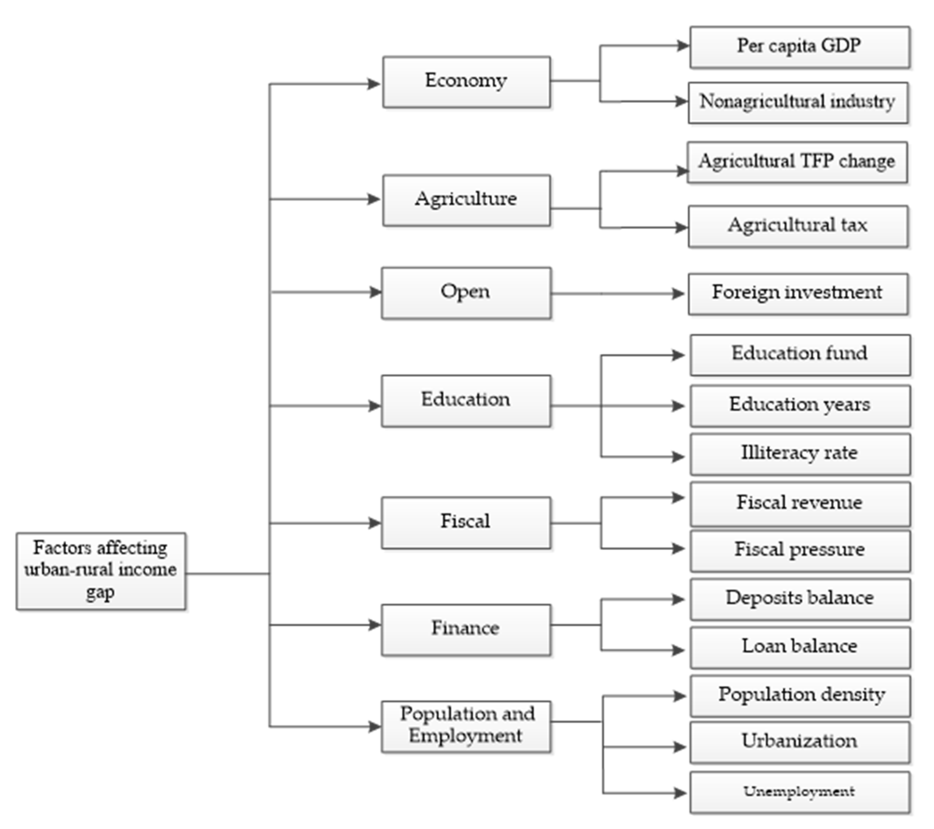
Construction of Variables Influencing the Rural–Urban Income Gap

The ratio of income between urban and rural residents adjusted by the CPI is used to directly measure the gap. In addition, we choose the Theil index as a proxy variable to measure the rural–urban income gap. The calculation formula of the Theil index is shown in Equation (21). Where T h e i l i t represents the Theil index value of province i in the year t, j = 1, 2 represents urban areas and rural areas, respectively, s i j , t represents the income of towns or farmers in region i in the year t, s i , t represents the total income of farmers in region i in the year t, r i j , t represents the urban or rural population in region i in the year t, and r i , t represents the total population in region i in the year t.
T h e i l i t = j = 1 J ( s i j , t s i , t ) L n ( s i j , t s i , t / r i j , t r i , t )
According to existing literature, there are many factors affecting the rural–urban income gap, and the core explanatory variables concerned in this article are the education level of farmers and the change in agricultural TFP. We take into account the existing relevant literature to build an indicator system affecting the rural–urban income gap. The system is mainly composed of 7 first-level indicators and 15 second-level indicators, as shown in Figure 2. The selected variables of the built indicator system are as follows:
  • Economy. The level and structure of economic development are reflected by the per capita real gross domestic product (RGDP) and the proportion of non-agricultural output, respectively [51].
  • Agriculture. We also took into account the agricultural development situation. Agricultural TFP change and agricultural tax are selected as agricultural development indicators [52].
  • Population and Employment. Population density, urbanization, and the unemployment rate are selected as secondary indicators. We use the proportion of urban residents to the total population as the measure of the urbanization rate [53,54].
  • Openness. The degree of China’s openness is measured by the share of foreign direct investment (FDI) in GDP. It is generally believed that the improvement of the opening level will widen the rural–urban income gap. However, this effect may also be altered by the export of agricultural products and the transfer of agricultural labor [5].
  • Education. In this paper, the share of government education expenditure in GDP, the education years of urban and rural residents, and the illiteracy rate of rural residents are selected as the secondary indicators to measure educational resources [27,55].
  • Fiscal. In China, the government plays an important role in economic and social activities, and its actions have a major impact on China’s economic development. On one hand, the government’s policy behavior can effectively promote economic development and significantly improve farmers’ income. On the other hand, urban policies have to a certain extent widened the income gap between urban and rural residents [56].
  • Finance. From the perspective of financial constraints, urban residents themselves have more abundant funds, compared with rural residents, so it is more likely for them to meet financial service conditions and enjoy high-yield returns. However, due to the threshold restrictions of financial services, it is not easy for rural residents to enjoy financial services, which will further widen income gap between urban and rural residents [6,57]. This paper selects the proportion of deposit balance and loan balance in GDP to represent the financial development level of each province.

Data Source and Descriptive Statistical Analysis

The data used in the empirical part of this paper are the province-level panel data of China covering the period from 2003 to 2017. The reason for choosing 30 provincial regions is the lack of relevant data in Tibet. So, the panel data contained 450 samples from 30 provinces for 15 consecutive years. The data were mainly from China Statistical Yearbooks, China Rural Statistical Yearbooks, and China Population and Employment Statistical Yearbooks from 2003 to 2018, as well as the official website of the People’s Bank of China. In addition, in order to eliminate the impact of price factors on the empirical results, this paper takes 2003 as the base period to flatten the variable of per capita GDP. Descriptive statistical analysis was conducted on variables by using Stata14.0, and the results are shown in Table 2.

3. Results

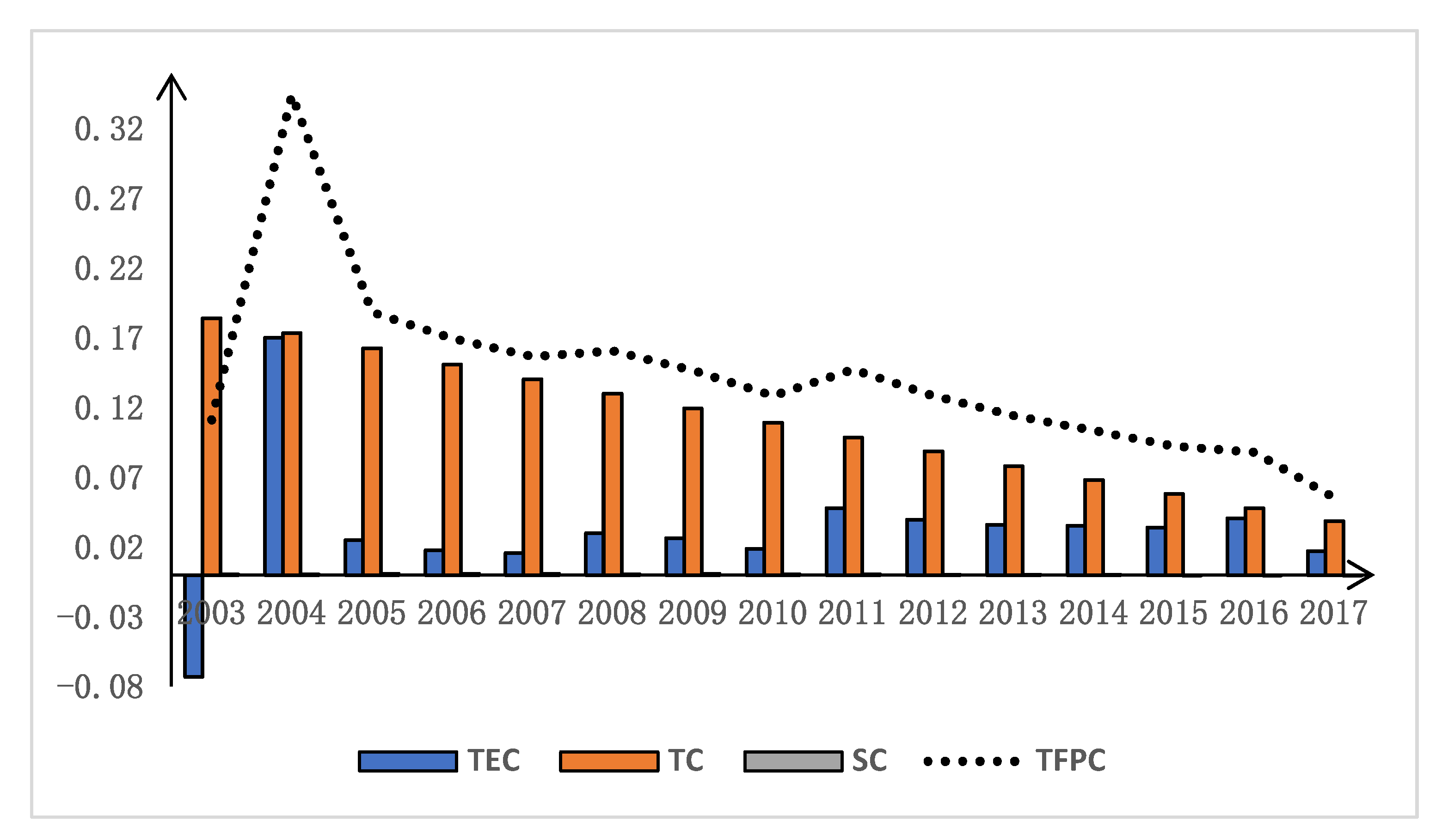
3.1. The Calculation of the Total Factor Productivity of Agriculture in China

Based on the study of Liu et al. [45], this paper calculates the concrete values of China’s agricultural TFP and its components by referring to the estimated results of the stochastic frontier model, in which the inefficiency term has a semi-normal distribution, from 2003 to 2017. We divide China’s agricultural total factor productivity into TEC, TC, and SC, and the results are shown in Figure 3.
Figure 3 shows that the change rate of China’s agricultural TFP is positive from 2003 to 2017, indicating that China’s agricultural productivity is constantly improving, which is consistent with the results calculated by Hu et al. [32]. From the perspective of agricultural TFP components, TC has the greatest impact on agricultural TFP [58], followed by TEC, while SC has almost no impact [30]. This shows that in China’s agricultural production, the return to scale has hardly changed, and the improvement of agricultural productivity is mainly driven by technological progress [30]. From the perspective of the time-change trend, the growth rate of agricultural TFP declined, mainly due to the decline of the TC growth rate. The TEC decreased significantly in 2003 and then rose rapidly in 2004, which was considered to be caused by the outbreak of SARS. From 2005 to 2010, the TEC showed a development trend of low growth, and then the growth rate increased after 2011.

3.2. The Effect of Farmers’ Education Level on the Rural–Urban Income Gap

Using the Stata 14.0 software, the model constructed from the panel data of 30 provinces in China from 2003 to 2017 was estimated by using the system GMM method. In order to show the consistency of the model estimation results, this paper, with reference to the existing literature [47], gives the OLS and fixed-effect model estimation results for coefficient comparison while conducting system GMM estimation of the model.
Taking into account the existence of unobservable individual effects, OLS estimation will cause the lag term coefficient of the explained variable to be higher, while the fixed-effect model estimation will lead to a lower lag term coefficient. Therefore, when the coefficient estimated by the system GMM is between the coefficient estimated by OLS and the coefficient estimated by the fixed-effect model, the estimated result is credible. To further analyze the robustness of the estimated results of the system GMM model, this paper considers reasonable replacement of the model by the explanatory variable (urban income/rural income), so the Theil Index is selected as the proxy variable of the explained variable. On this basis, the new explained variable is used to estimate the system GMM of the model and verify the robustness of the results.
Table 3 shows the estimated results of the impact of farmers’ education level on the rural–urban income gap. Among them, model (a) and (c) respectively represent the estimation results of Equation (15) under the three models of ordinary least squares (OLS), the fixed-effect model (FE), and the system GMM. Model (d) replaces the explained variable with the Theil index as a robustness test.
The estimation results show that the lag term coefficient of the explanatory variable obtained by the system GMM estimation method is 0.8665, which indeed lies between the OLS estimation result (0.9454) and the fixed-effect model estimation result (0.8455), indicating that the result of the system GMM estimation method is reasonable. The coefficient of the lag period of the rural–urban income gap is positive and significant at the 1% level, so it can be inferred that the rural–urban income gap has a certain persistent effect and growth inertia. At the same time, both AR(2) and Sargan statistics cannot reject the existence of second-order autocorrelation and all instrumental variations of the model residences. The null hypothesis that the quantities are all valid indicates that the model setting is appropriate. Specifically, the coefficient of the illiteracy rate of farmers and its impact on the rural–urban income gap is positive and significant at the 1% confidence level, indicating that the improvement of farmers’ education level will reduce the rural–urban income gap. In order to test the robustness of this conclusion, the last column of Table 3 presents the estimated results after replacing the explained variable. It is found that the illiteracy rate of farmers still has a positive impact on the rural–urban income gap, indicating that the conclusion is robust. From another perspective, that is to say, increasing the input of educational resources in rural areas and improving the educational level of farmers will help increase farmers’ income, thereby maintaining social equity and justice and narrowing the rural–urban income gap.
According to the estimated results of the control variables, the coefficient of RGDP is significantly negative, indicating that during the sample period, the improvement of economic growth is conducive to narrowing the income gap between urban and rural residents, which is consistent with the findings of Tang et al. [59] and Chen and Lin [3]. This can be explained as follows: the more developed the economy is, the more capable the region is in promoting the increase of farmers’ income and narrowing urban–rural income gap. The coefficient of the proportion of non-agricultural industries is significantly positive, indicating that the higher the proportion of non-agricultural industries, the greater the rural–urban income gap. The main reason is that farmers are not well-educated and are in a relatively weak position in the job market, so it is difficult for them to seek high-paying jobs in the job market. Therefore, improvement of the industrialization level has widened the rural–urban income gap. The coefficient of financial pressure is positive, indicating the increase of financial pressure contributes to a larger rural–urban income gap. A possible reason is that increasing financial pressure makes it more difficult to increase fiscal expenditures, which is not conducive to improving farmers’ income, thus widening the rural–urban income gap. FDI has a significant inhibiting effect on the rural–urban income gap, which may be attributed to the employment effect of foreign investment. With the continuous improvement of economic openness, the pace of inward migration of labor-intensive industries is accelerated, so agricultural migrant workers obtain a large number of job opportunities, which is conducive to narrowing the rural–urban income gap [20]. The increase of residents’ years of education will widen the rural–urban income gap, and the reason may be related to the gap in the educational levels of urban and rural residents. The increase in the number of years of education is more likely to be caused by the behavior of urban residents, which will further increase the education levels of urban and rural residents and widen the income gap. As the rural economy is relatively backward, the highly educated rural labor force is more likely to migrate to cities and towns and become urban residents, which will further widen the rural–urban income gap. The proportion of loan balance to GDP has a significantly negative impact on the rural–urban income gap. A possible reason is that the greater the loan balance, the greater the possibility of financial support for rural residents, which is conducive to improving farmers’ income.

3.3. The Effect of Farmer’s Education Level on Agricultural TFP

According to the model setting, this part analyzes the influence of the education level of farmers on agricultural TFP. In addition, this part analyzes the effects of the education level of farmers on different components of TFP, and the results are shown in Table 4. The estimation results of the model show that the effect of farmers’ illiteracy rate on TFP is statistically significant and negative, that is, the improvement of farmers’ education level is conducive to the increase of agricultural TFP. From the perspective of the different components of TFP, farmers’ illiteracy rate has a significant and negative impact on TE and TEC, but does not have a significant impact on scale efficiency. Specifically, the impact on TEC is greater than that on TC. According to the estimated results of the control variables, the government’s comprehensive agricultural project development investment and the rate of agricultural irrigation significantly promoted the growth of agricultural TFP. However, the per capita savings of rural households, fiscal expenditure on agriculture, forestry and water affairs, aging ratio, and agricultural disaster rate are not conducive to the growth of agricultural TFP.

3.4. The Effect of Farmer’s Education Level and Agricultural TFP on the Rural–Urban Income Gap

Table 5 shows the estimated results of Equation (17). It can be found that the p-values of the AR(2) test and Hansen test of Model (iii) are both significantly greater than 0.1, and the estimated results of the lag term coefficients of the explained variables are located between the estimation results of Model (i) and Model (ii), indicating that the set econometric model and the selected estimation method are reasonable.
According to the estimation results of the variables, both the illiteracy rate of farmers and agricultural TFP have a significant impact on the rural–urban income gap. Combined with the above analysis, it is shown that the agricultural TFP does play a mediating role in the impact of the farmers’ education level on the rural–urban income gap. The improvement of the education level of farmers not only plays a direct role in narrowing the income gap between urban and rural areas, but also it can indirectly narrow the rural–urban income gap by increasing agricultural TFP.
In order to further analyze the effects of the various components of TFP and the illiteracy rate of farmers on the rural–urban income gap, the agricultural TFP in Equation (17) is replaced with TEC, TC, and SC, and re-estimated using the system GMM method. The results are shown in Table 6.
The estimation results in Table 6 show that the coefficient of TEC is significantly negative, while the coefficients of TC and SC are not significant. Combining the results with the information in Table 4 above, the illiteracy rate of farmers has a significant impact on both TEC and TC. Therefore, the improvement of the education level of farmers can narrow the rural–urban income gap through the intermediary effect of agricultural technology efficiency. Then, we analyze the mediating role of agricultural TC. The estimation result of Model (2) shows that the coefficient of TC is not significant. Therefore, progress of agricultural technology has a completely mediating effect.

3.5. Interaction of Farmers’ Education Level and Agricultural TFP Regarding the Rural–Urban Income Gap

According to different situations under the interaction effect of the education level of farmers and the change of agricultural TFP and how they impact the rural–urban income gap, four models were constructed above to represent the emerging situations. Table 7 shows the estimated results of the four models.
In general, the estimated results show that the model can pass AR(2) and Sargan tests, indicating the model setting is reasonable. The regression results are shown in the first column of Table 7, when the rural–urban income gap is not affected by the education level of farmers and agricultural TFP. When the rural–urban income gap is affected by the education level of farmers but not by agricultural TFP, it is consistent with the model in Equation (15), and the estimated results are shown in Model (c) in Table 3. When the rural–urban income gap is influenced by agricultural TFP but not by the education level of farmers, the estimated results for Case 2 are shown in Model (ii) in Table 7. The coefficient of agricultural TFP is significantly negative, indicating that the increase of agricultural TFP can effectively reduce the rural–urban income gap. Specifically, the income gap between urban and rural areas was reduced by 0.4561 for each 1-point increase in agricultural TFP, which may be because the increase of agricultural TFP is conducive to the increase of farmers’ income, thus narrowing the rural–urban income gap.
It can be seen that the increase of agricultural TFP and the improvement of farmers’ education level both have a significant impact on narrowing the rural–urban income gap. Considering that the education level of farmers and the change of agricultural TFP are not independent of each other, the interaction effect between the two is further investigated, and the interaction term of the two (TFP change * illiteracy rate) is included in the model to correspond to the estimation result of Model (iv) in Table 7. It can be seen from the estimation results of the model that the interaction term is significant at the level of 10% and the sign is positive, indicating that the interaction effect between the illiteracy rate of farmers and the change of agricultural TFP widens the rural–urban income gap. In other words, the increase of agricultural TFP enlarges the marginal effect of the education level of farmers on the rural–urban income gap. Meanwhile, the improvement of the education level of farmers enlarges the marginal effect of agricultural TFP on the rural–urban income gap.
The reasons for the above results can be derived from the source of the increase in agricultural TFP. Through the analysis of the sources of China’s agricultural TFP growth above, it can be found that the growth of China’s agricultural TFP mainly comes from the progress of agricultural technology. [58] also showed that the agricultural TFP in China, to a large extent, reflects the change in agricultural technological progress. This implies a higher requirements for farmers’ production technology level, and farmers need to have higher professional skills to match advanced agricultural technology. Therefore, when the education level of farmers increases, the marginal effect of agricultural TFP on the rural–urban income gap will be further amplified.

3.6. Quantile Regression Analysis of Farmers’ Education Level, Agricultural TFP, and the Rural–Urban Income Gap

Quantile regression analysis describes how the independent variable affects the different quantiles of the dependent variable. At different quantile levels, the parameter coefficient represents the effect of the same influencing factor on the dependent variable [60,61]. This paper analyzes the effects of agricultural TFP and the education level of farmers on the rural–urban income gap under different quantiles, and the results are shown in Table 8. For simplicity, we report only the results estimated at the 10th, 25th, 50th, 75th, and 90th quantiles. The estimation results in Table 8 show that, at each quantile level, the increase of farmers’ education level significantly narrows the rural–urban income gap, but its coefficients are different at different quantiles. Figure 4 shows the coefficient of the farmer illiteracy rate and its 95% confidence interval at different quantiles. At the 75th quantile level, the illiteracy rate of farmers has the greatest impact on the rural–urban income gap. When the illiteracy rate of farmers is reduced by one percentage point, the rural–urban income gap is reduced by 0.0329.
It can be found that with the increase of the quantile, the effect of the education level of farmers on the rural–urban income gap generally presents a downward trend. A possible reason is that when the rural–urban income gap is at a lower quantile, that is, when the rural–urban income gap is small, farmers may have part-time jobs. Farmers’ non-agricultural wage income accounts for a relatively high proportion of their total income, and non-agricultural work also requires relatively high overall quality of farmers. Therefore, the education level of farmers has a greater impact on the rural–urban income gap at low quantiles.
From the perspective of the impact of agricultural TFP on the rural–urban income gap, the impact of agricultural TFP on the rural–urban income gap is not significant at lower levels. However, the increase of agricultural TFP can reduce the rural–urban income gap at higher levels. This paper considers that the possible reasons lie in the different sources of farmers’ income. At high levels of the rural–urban income gap, the main income of farmers comes from agricultural production [62], so the increase of agricultural TFP is conducive to promoting farmers’ income, which narrows the rural–urban income gap.

4. Conclusions

Based on the panel data of 30 provinces in China from 2003 to 2017, this paper first analyzed the impact of the education level of farmers on the rural–urban income gap as well as the mediating role of agricultural TFP. Subsequently, an interaction effect model was constructed to study the interaction effect of farmers’ education level and agricultural TFP on the rural–urban income gap. Finally, under different quantiles, the paper studied the differential impact of the education level of farmers and agricultural TFP on the rural–urban income gap. The main conclusions of this study can be drawn as follows.
The education level of farmers can not only affect the rural–urban income gap directly, but also affect the agricultural TFP to have an indirect impact on the rural–urban income gap. To a certain extent, the education level of farmers can represent the labor skills of farmers. An increase in the education level of farmers indicates improvement of the quality of farmers’ labor force; in this situation, farmers are more likely to engage in higher-paying non-agricultural work, thus increasing their non-agricultural income and narrowing the rural–urban income gap. In addition, an increase in the education level of farmers enables farmers to master new agricultural technologies, thereby effectively promoting the improvement of agricultural TFP. Therefore, greater education can improve farmers’ agricultural income and the narrow rural–urban income gap.
Agricultural TFP and the education level of farmers are not independent of each other, but interactive. The interaction effect has significantly widened rural–urban income gap. An increase of agricultural TFP will enlarge the marginal effect of the education level of farmers on the rural–urban income gap, and an increase of the education level of farmers will also increase the impact of agricultural TFP on the rural–urban income gap.
The education level of farmers and agricultural TFP have different impacts on the rural–urban income gap at different quantiles. From the perspective of the effect of the education level of farmers, the coefficient of influence decreases as the rural–urban income gap increases. From the perspective of the impact of agricultural TFP, the impact coefficient is only significant at the high quantile of the rural–urban income gap. This may be caused by differences in the composition of farmers’ income in different regions.
Based on the above conclusions, the following policy recommendations are proposed to narrow the rural–urban income gap. First, the Chinese government should further increase primary education of the adult rural labor force, including the elderly. On the one hand, it is helpful to engage new professional farmers who will become “educated” and “skilled”. On the other hand, it can widen the range of employment opportunities and will not require farmers to remain engaged in simple, physically demanding work. Obviously, these two aspects can improve farmers’ income in the long term and short term, respectively. Second, we propose to vigorously develop adult education in rural areas and improve the vocational education level of migrant workers. Vocational education plays an indispensable role in the process of increasing the income of migrant workers. Agricultural modernization, mechanization, and intellectualization promote technological progress and TFP growth. Vigorously developing rural adult education can improve farmers’ education level and adapt modern agricultural production practices. This just shows that farmers’ income can be increased through the growth of agricultural TFP and the increase of output. Third, to strengthen the training of farmers, it would be wise to adopt advanced agricultural production technology and improve agricultural TFP. The improvement of agricultural TFP is not only conducive to the sustainable development of agriculture, but also conducive to the release of part of the rural labor force and the upgrading of industrial structure. The released rural surplus labor can engage in other non-agricultural work, which will promote the increase of farmers’ non-agricultural income and narrow the rural–urban income gap. Therefore, on one hand, the government should increase technical training for farmers to improve their professional skills. On the other hand, farmers should take the initiative to strengthen their own learning and improve their abilities. Fourth, it is necessary to adapt measures to local conditions and implement differentiated policies for the current rural–urban income gap in different regions. For areas with large rural–urban income gaps, it is necessary to strengthen training of farmers’ agricultural production techniques and improve agricultural TFP to narrow the rural–urban income gap. For areas with relatively small rural–urban income gaps, it is necessary to strengthen the education and training of farmers, which can further narrow the rural–urban income gap.
This study also has some limitations. First of all, with the continuous promotion and development of China’s compulsory education and the continuous improvement of science and technology, it may no longer match the social reality to use the illiteracy rate to represent the education level of farmers. Secondly, agricultural digital transformation plays an important role in improving agricultural productivity [63] and increasing farmers’ income [64]. The education level of farmers may have a direct impact on the digitization of the agricultural industry. In a future study, we can use the proportion of education to represent the level of education and also consider the impact of different levels of education on the urban–rural income gap. How to narrow the urban–rural income gap through agricultural industry digitization and education level improvement is also an interesting research question.

Author Contributions

Conceptualization, J.L. and S.L.; methodology, J.L. and X.L.; software, X.L.; validation, S.S. and X.L.; resources, J.L.; data curation, S.L.; writing—original draft preparation, S.L.; writing—review and editing, J.L. and S.R.; visualization, X.L.; supervision, S.R.; project administration, J.L.; funding acquisition, S.S. All authors have read and agreed to the published version of the manuscript.

Funding

This research received no external funding.

Institutional Review Board Statement

Not applicable.

Informed Consent Statement

Not applicable.

Data Availability Statement

All data can be obtained by email from the corresponding author.

Acknowledgments

This work has been assisted by the China–ASEAN High-Quality Development Research Center at Shandong University of Finance and Economics and the “Theoretical Economics Research Innovation Team” of the Youth Innovation Talent Introduction and Education Plan of Colleges and Universities in Shandong Province for financial support, as well as the Faculty of Economics and the Centre of Excellence in Econometrics at Chiang Mai University.

Conflicts of Interest

The authors declare no conflict of interest.

References

  1. Berisha, E.; Meszaros, J. Macroeconomic determinants of wealth inequality dynamics. Econ. Model. 2020, 89, 153–165. [Google Scholar] [CrossRef]
  2. Chu, L.K.; Hoang, D.P. How does economic complexity influence income inequality? New evidence from international data. Econ. Anal. Policy 2020, 68, 44–57. [Google Scholar] [CrossRef]
  3. Chen, B.K.; Lin, Y.F. Development strategy, urbanization and the rural-urban income gap in China. Soc. Sci. China 2014, 35, 5–20. [Google Scholar]
  4. Wang, S.L.; Tan, S.K.; Yang, S.F.; Lin, Q.W.; Zhang, L. Urban-biased land development policy and the rural-urban income gap: Evidence from Hubei Province, China. Land Use Policy 2019, 87, 104066. [Google Scholar] [CrossRef]
  5. Wang, X.; Shao, S.; Li, L. Agricultural inputs, urbanization and rural-urban income disparity: Evidence from China. China Econ. Rev. 2019, 55, 67–84. [Google Scholar] [CrossRef]
  6. Su, C.W.; Song, Y.; Ma, Y.T.; Tao, R. Is financial development narrowing the rural-urban income gap? A cross-regional study of China. Pap. Reg. Sci. 2019, 98, 1779–1800. [Google Scholar] [CrossRef]
  7. Su, Y.F.; Lau, C.; Rao, N. Early education policy in China: Reducing regional and socioeconomic disparities in preschool attendance. Early Child. Res. Q. 2020, 53, 11–22. [Google Scholar] [CrossRef]
  8. Zhang, H.F. Opportunity or new poverty trap: Rural-urban education disparity and internal migration in China. China Econ. Rev. 2017, 44, 112–124. [Google Scholar] [CrossRef]
  9. Su, B.W.; Heshmati, A. Analysis of the determinants of income and income gap between urban and rural China. China Econ. Policy Rev. 2013, 2, 1350002. [Google Scholar] [CrossRef] [Green Version]
  10. Zachariadis, M.; Savvides, A. International Technology Diffusion and the Growth of TFP in the Manufacturing Sector of Developing Economies. Rev. Dev. Econ. 2005, 9, 482–501. [Google Scholar]
  11. Luo, C.L.; Li, S.; Sicular, T. The long-term evolution of national income inequality and rural poverty in China. China Econ. Rev. 2020, 62, 101465. [Google Scholar] [CrossRef]
  12. Chen, L.L.; Shen, W. Spatiotemporal differentiation of rural-urban income disparity and its driving force in the Yangtze River Economic Belt during 2000–2017. PLoS ONE 2021, 16, e0245961. [Google Scholar] [CrossRef] [PubMed]
  13. Ma, Y.; Chen, D. Openness, rural-urban inequality, and happiness in China. Economic Systems. Econ. Syst. 2020, 44, 100834. [Google Scholar] [CrossRef]
  14. Wang, M.; Kang, W.M.; Zhang, R.Y. The gap between urban and rural development levels narrowed. Complexity 2020, 2020, 4615760. [Google Scholar] [CrossRef]
  15. Song, H.Y.; Ma, Y.L. An estimation of the rural-urban gap in China using the Human Development Index. Econ. Res. 2004, 11, 4–15. [Google Scholar]
  16. Gradín, C.; Wu, B.B. Income and consumption inequality in China: A comparative approach with India. China Econ. Rev. 2020, 62, 101463. [Google Scholar] [CrossRef]
  17. Li, S.; Luo, C.L. Re-estimating the income gap between urban and rural households in China. Procedia-Soc. Behav. Sci. 2010, 2, 7151–7163. [Google Scholar]
  18. Ji, X.; Wang, K.; Xu, H.; Li, M. Has Digital Financial Inclusion Narrowed the Urban-Rural Income Gap: The Role of Entrepreneurship in China. Sustainability 2021, 13, 8292. [Google Scholar] [CrossRef]
  19. Zhong, S.J.; Wang, M.S.; Zhu, Y.; Chen, Z.G.; Huang, X.J. Urban expansion and the urban-rural income gap: Empirical evidence from China. Cities 2022, 129, 103831. [Google Scholar] [CrossRef]
  20. Zhu, S.J.; Yu, C.D.; He, C.F. Export structures, income inequality and rural-urban divide in China. Appl. Geogr. 2020, 115, 102150. [Google Scholar] [CrossRef]
  21. Chen, Y.G.; Luo, P.; Chang, T. Urbanization and the urban-rural income gap in China: A continuous wavelet coherency analysis. Sustainability 2020, 12, 8261. [Google Scholar] [CrossRef]
  22. Weng, Y.Z.; Zeng, Y.T.; Lin, W.S. Do rural highways narrow Chinese farmers’ income gap among provinces? J. Integr. Agric. 2021, 20, 905–914. [Google Scholar] [CrossRef]
  23. Wang, S.L.; Huang, J.K.; Wang, X.B.; Tuan, F. Are China’s regional agricultural productivities converging: How and why? Food Policy 2019, 86, 101727. [Google Scholar] [CrossRef]
  24. Yuan, Y.; Wang, M.S.; Zhu, Y.; Huang, X.J.; Xiong, X.F. Urbanization’s effects on the rural-urban income gap in China: A meta-regression analysis. Land Use Policy 2020, 99, 104995. [Google Scholar] [CrossRef]
  25. Li, Y.C.; Wang, X.P.; Zhu, Q.S.; Zhao, H. Assessing the spatial and temporal differences in the impacts of factor allocation and urbanization on urban-rural income disparity in China, 2004–2010. Habitat Int. 2014, 42, 76–82. [Google Scholar] [CrossRef]
  26. Lessmann, C.; Seidel, A. Regional inequality, convergence and its determinants—A view from outer space. Eur. Econ. Rev. 2017, 92, 110–132. [Google Scholar] [CrossRef] [Green Version]
  27. Anlimachie, M.A.; Avoada, C. Socio-economic impact of closing the rural-urban gap in pre-tertiary education in Ghana: Context and strategies. Int. J. Educ. Dev. 2020, 77, 102236. [Google Scholar] [CrossRef]
  28. Alves, L.G.A.; Andrade, J.S.; Hanley, Q.S.; Ribeiro, H.V. The hidden traits of endemic illiteracy in cities. Phys. A Stat. Mech. Its Appl. 2019, 515, 566–574. [Google Scholar] [CrossRef] [Green Version]
  29. Gao, Y.Y.; Zang, L.Z.; Sun, J. Does computer penetration increase farmers’ income? An empirical study from China. Telecommun. Policy 2018, 42, 345–360. [Google Scholar] [CrossRef]
  30. Shen, Z.Y.; Baležentis, T.; Ferrier, G.D. Agricultural productivity evolution in China: A generalized decomposition of the Luenberger-Hicks-Moorsteen productivity indicator. China Econ. Rev. 2019, 57, 101315. [Google Scholar] [CrossRef]
  31. Han, W.; Wei, Y.G.; Cai, J.M.; Yu, Y.J.; Chen, F.R. Rural nonfarm sector and rural residents’ incomeresearch in China. An empirical study on the township and village enterprises after ownership reform (2000–2013). J. Rural Stud. 2021, 82, 161–175. [Google Scholar] [CrossRef]
  32. Hu, Y.; Liu, C.; Peng, J.G. Financial inclusion and agricultural total factor productivity growth in China. Econ. Model. 2021, 96, 68–82. [Google Scholar] [CrossRef]
  33. Wang, C.; Deng, M.Z.; Deng, J.F. Factor reallocation and structural transformation implications of grain subsidies in China. J. Asian Econ. 2020, 71, 101248. [Google Scholar] [CrossRef]
  34. Li, Q.; Wu, X.H.; Zhang, Y.; Wang, F.Y. The effect of agricultural environmental total factor productivity on rural-urban income gap: Integrated view from China. Sustainability 2020, 12, 3327. [Google Scholar] [CrossRef]
  35. Tan, Y.T.; Xu, H.; Zhang, X.L. Sustainable urbanization in China: A comprehensive literature review. Cities 2016, 55, 82–93. [Google Scholar] [CrossRef]
  36. Rada, N.; Helfand, S.; Magalhães, M. Agricultural productivity growth in Brazil: Large and small farms excel. Food Policy 2019, 84, 176–185. [Google Scholar] [CrossRef]
  37. Liu, J.; Dong, C.; Liu, S.; Rahman, S.; Sriboonchitta, S. Sources of total-factor productivity and efficiency changes in China’s agriculture. Agriculture 2020, 10, 279. [Google Scholar] [CrossRef]
  38. Zhang, C.; Hu, R. Does Fertilizer Use Intensity Respond to the Urban-Rural Income Gap? Evidence from a Dynamic Panel-Data Analysis in China. Sustainability 2020, 12, 430. [Google Scholar] [CrossRef] [Green Version]
  39. Huang, Y.X.; Zhang, Y. Financial Inclusion and Urban-Rural Income Inequality: Long-Run and Short-Run Relationships. Emerg. Mark. Financ. Trade 2019, 56, 457–471. [Google Scholar] [CrossRef]
  40. Yuan, B.; Li, C.; Xiong, X. Innovation and environmental total factor productivity in China: The moderating roles of economic policy uncertainty and marketization process. Env. Sci. Pollut. Res. 2021, 28, 9558–9581. [Google Scholar] [CrossRef]
  41. Liu, J.; Rahman, S.; Sriboonchitta, S.; Wiboonpongse, A. Enhancing Productivity and Resource Conservation by Eliminating Inefficiency of Thai Rice Farmers: A Zero Inefficiency Stochastic Frontier Approach. Sustainability 2017, 9, 770. [Google Scholar] [CrossRef] [Green Version]
  42. Coelli, T.J. Recent Development in Frontier Modeling and Efficiency Measurement. Aust. J. Agric. Econ. 1995, 39, 219–245. [Google Scholar]
  43. Laureti, T.; Benedetti, I.; Branca, G. Water use efficiency and public goods conservation: A spatial stochastic frontier model applied to irrigation in Southern Italy. Socio-Econ. Plan. Sci. 2021, 73, 100856. [Google Scholar] [CrossRef]
  44. Kumbhakar, S.C.; Lovell, C.A.K. Stochastic Frontier Analysis; Cambridge University Press: Cambridge, UK, 2000; pp. 279–309. [Google Scholar]
  45. Liu, J.; Wang, M.; Yang, L.; Rahman, S.; Sriboonchitta, S. Agricultural productivity growth and its determinants in South and Southeast Asian countries. Sustainability 2020, 12, 4981. [Google Scholar] [CrossRef]
  46. Ullah, S.; Akhtar, P.; Zaefarian, G. Dealing with endogeneity bias: The generalized method of moments (GMM) for panel data. Ind. Mark. Manag. 2018, 71, 69–78. [Google Scholar] [CrossRef]
  47. Arellano, M.; Bond, S. Some tests of specification for panel data: Monte carlo evidence and an application to employment equations. Rev. Econ. Stud. 1991, 58, 277–298. [Google Scholar] [CrossRef] [Green Version]
  48. Blundell, R.; Bond, S. Initial conditions and moment restrictions in dynamic panel data models. J. Econom. 1998, 87, 115–143. [Google Scholar] [CrossRef] [Green Version]
  49. Mittal, A.; Garg, A.K. Bank stocks inform higher growth-A System GMM analysis of ten emerging markets in Asia. Q. Rev. Econ. Financ. 2021, 79, 210–220. [Google Scholar] [CrossRef]
  50. Rahman, S.; Salim, R. Six decades of total factor productivity change and sources of growth in Bangladesh agriculture. J. Agric. Econ. 2013, 64, 275–294. [Google Scholar] [CrossRef] [Green Version]
  51. Zeng, C.; Song, Y.; He, Q.; Liu, Y. Urban-rural income change: Influences of landscape pattern and administrative spatial spillover effect. Appl. Geogr. 2018, 97, 248–262. [Google Scholar] [CrossRef]
  52. Wang, X.; Shen, Y. The effect of China’s agricultural tax abolition on rural families’ incomes and production. China Econ. Rev. 2014, 29, 185–199. [Google Scholar] [CrossRef]
  53. Dong, X.; Hao, Y. Would income inequality affect electricity consumption? Evidence from China. Energy 2018, 142, 215–227. [Google Scholar] [CrossRef]
  54. Su, C.; Liu, T.; Chang, H.; Jiang, X. Is urbanization narrowing the rural-urban income gap? A cross-regional study of China. Habitat Int. 2015, 48, 79–86. [Google Scholar] [CrossRef]
  55. Lu, D. Rural-urban income disparity: Impact of growth, allocative efficiency and local growth welfare. China Econ. Rev. 2002, 13, 419–429. [Google Scholar] [CrossRef]
  56. Chen, X.; Zhang, X.; Song, Y.; Liang, X.; Wang, L.; Geng, Y. Fiscal decentralization, rural-urban income gap and tourism. Sustainability 2020, 12, 10398. [Google Scholar] [CrossRef]
  57. Seven, Ü. Finance, talent and income inequality: Cross-country evidence. Borsa Istanb. Rev. 2022, 22, 57–68. [Google Scholar] [CrossRef]
  58. Sheng, Y.; Tian, X.; Qiao, W.; Peng, C. Measuring agricultural total factor productivity in China: Pattern and drivers over the period of 1978–2016. Aust. J. Agric. Resour. Econ. 2020, 64, 82–103. [Google Scholar] [CrossRef]
  59. Tang, J.J.; Gong, J.W.; Ma, W.L.; Rahut, D.B. Narrowing urban-rural income gap in China: The role of the targeted poverty alleviation program. Econ. Anal. Policy 2022, 75, 74–90. [Google Scholar] [CrossRef]
  60. Koenker, R.; Bassett, G., Jr. Regression quantiles. Econom. J. Econom. Soc. 1978, 46, 33–50. [Google Scholar] [CrossRef]
  61. Koenker, R. Quantile regression for longitudinal data. Multivar. Anal. 2004, 91, 74–89. [Google Scholar] [CrossRef] [Green Version]
  62. Li, Y.; Wang, Z. Analysis on the effect of farmer income of policy-based agricultural insurance. Acta Agric. Scand. Sect. B-Soil Plant Sci. 2022, 72, 386–400. [Google Scholar] [CrossRef]
  63. Zhou, Z.; Liu, W.; Wang, H.; Yang, J. The Impact of Environmental Regulation on Agricultural Productivity: From the Perspective of Digital Transformation. Int. J. Environ. Res. Public Health 2022, 19, 10794. [Google Scholar] [CrossRef] [PubMed]
  64. Chen, W.; Wang, Q.; Zhou, H. Digital Rural Construction and Farmers’ Income Growth: Theoretical Mechanism and Micro Experience Based on Data from China. Sustainability 2022, 14, 11679. [Google Scholar] [CrossRef]
Figure 1. The effect of farmers’ education level on the rural–urban income gap based on the mediating effect of agricultural TFP.
Agriculture 12 01920 g001
Figure 2. Indicators to identify determinants of the rural–urban income gap.
Agriculture 12 01920 g002
Figure 3. TFP change and its decomposition changes from 2003 to 2017.
Agriculture 12 01920 g003
Figure 4. The coefficient of the illiteracy rate under quantile regression.
Agriculture 12 01920 g004
Table 1. Models under different circumstances affecting rural–urban income gap.
Not Affected by TFP ChangeAffected by TFP Change
Not affected by farmers’ educationCase 1. Model (i)Case 2. Model (ii)
Affected by farmers’ educationCase 3. Model (iii)Case 4. Model (iv)
Table 2. Descriptive statistics.
VariableUnitMeanStandard DeviationMinMax
I. Rural–urban income gap
Urban income/rural incomeRatio2.9660.5471.8454.771
II. Factors affecting agricultural output
Agricultural output108 Yuan1130.4431047.4813.95174.9
Labor input104 Person993.6597717.92534.623398
Planting area103 Ha5304.8283590.794120.9414,902.72
Machinery power104 Kilowatt2858.5952736.30895.3213,353.02
Plastic film104 Ton7.09926.43870.082134.3524
Pesticide104 Ton5.4474584.3251830.1617.35
III. Factors affecting rural–urban income gap
Illiteracy ratePercent7.16074.49891.2324.07
Per capita GDP104 Yuan2.66721.83840.370110.4133
Non-agricultural Percent88.41856.131462.987299.6384
Fiscal revenuePercent14.534.280378.132.7
Fiscal pressure-2.24200.93861.05166.7450
UrbanPercent51.194814.454419.8589.6
Population108 person286.81961002.4420.05334622.064
UnemploymentPercent3.58100.69261.216.5
OpenPercent41.200651.42004.8067585.7918
Tax-0.73330.442701
Education fundPercent4.91101.48572.477310.3802
Education yearsyear8.68201.04136.040412.7653
Deposits balancePercent1.62320.70630.75095.5865
Loan balancePercent1.16310.42900.28772.5847
Table 3. The influence of farmers’ education level the on rural–urban income gap.
Model (i)Model (ii)Model (iii)Model (iv)
OLSFESystem
GMM
Robustness
L.income gap0.9454 ***0.8455 ***0.8665 ***0.4338 ***
(0.0192)(0.0277)(0.0493)(0.0498)
Illiteracy rate0.0118 ***0.0196 ***0.0299 *** 0.0024 ***
(0.0029)(0.0035)(0.0028)(0.0003)
RGDP−0.0083−0.0062−0.0245 ***0.0316 ***
(0.0060)(0.0101)(0.0088)(0.0059)
Non-agricultural0.0003−0.00230.0074 *0.0035 ***
(0.0013)(0.0033)(0.0042)(0.0005)
Fiscal revenue−0.0018−0.0029−0.0047−0.0030 ***
(0.0021)(0.0047)(0.0029)(0.0007)
Financial pressure0.0008
(0.0077)
0.0143
(0.0267)
0.0477 **
(0.0242)
−0.0223 ***
(0.0037)
Urban−0.0009
(0.0009)
−0.0019
(0.0013)
0.0004
(0.0009)
−0.0105 ***
(0.0020)
Population 4.23 × 10⁻⁶
(3.97 × 10⁻⁶)
0.00008
(0.0001)
0.0001
(0.0001)
−0.00007 **
(0.00003)
Unemployment0.0086
(0.0073)
0.0048
(0.0189)
0.0019
(0.0176)
0.0396 ***
(0.0063)
Open0.0002 ***0.00001−0.0001 *−0.00002 ***
(0.00007)(0.0001)(0.0001)(9.48 × 10⁻⁶)
Tax−0.0356 **0.02660.0129−0.0023
(0.0151)(0.0198)(0.0118)(0.0021)
Education years0.0481 ***0.01600.0773 ***−0.0080 ***
(0.0168)(0.0238)(0.0151)(0.0030)
Deposits balance0.01630.04037270.1052 *0.0263 **
(0.0154)(0.0418)(0.0584)(0.0127)
Loan balance−0.0357−0.0507−0.2158 **−0.0580 ***
(0.0241)(0.0441)(0.0935)(0.0155)
Constant−0.2931 *0.4319−1.1640 ***0.3303 ***
(0.1752)(0.4020)(0.3879)(0.1191)
R20.96980.8731
F-statistic756.30350.88
Wald test (chi2) 3713.7241064.03
Wald test (p-value) 0.00000.0000
Sargan test (chi2) 27.022722.9966
Sargan test (p-value) 0.88590.9652
Arellano-Bond test for AR(1)
(z-statistic) −3.569−1.0786
(p-value) 0.00040.2808
Arellano-Bond test for AR(2)
(z-statistic) −0.2081−0.6804
(p-value) 0.83510.4962
t statistics in parentheses; * p < 0.1, ** p < 0.05, *** p < 0.01.
Table 4. The influence of farmers’ illiteracy on the TFP change.
TFP ChangeTCTECSC
Constant−0.3861 *
(0.2021)
0.1402 ***
(0.0227)
−0.5291 ***
(0.2006)
0.0027 ***
(0.0008)
Illiteracy rate−0.0042 **
(0.0018)
−0.0011 ***
(0.0002)
−0.0030 *
(0.0018)
−0.00001
(0.00001)
Saving−0.0733 ***
(0.0186)
−0.0448 ***
(0.0022)
−0.0281
(0.0181)
−0.0003 ***
(0.0001)
Size0.0362
(0.0269)
−0.0049
(0.0053)
0.0412
(0.0274)
−0.0001
(0.0001)
Expenditure−0.0283 ***
(0.0107)
−0.0202 ***
(0.0016)
−0.0080
(0.0104)
0.00001
(0.0001)
Development0.0623 ***
(0.0202)
0.0093 ***
(0.0019)
0.0530 ***
(0.0200)
−0.00007
(0.00009)
Disaster−0.1267 ***
(0.0403)
0.0032
(0.0084)
−0.1314 ***
(0.0400)
0.0014 **
(0.0006)
Irrigation0.1805 ***
(0.0652)
0.0013
(0.0078)
0.1798 ***
(0.0627)
−0.0006 *
(0.0003)
Population−0.0016
(0.0013)
0.0001
(0.0003)
−0.0016
(0.0012)
−0.00004 **
(0.00001)
Older−0.4808 **
(0.2251)
0.0693 *
(0.0395)
−0.5422 **
(0.2248)
−0.0079 ***
(0.0019)
R-squared0.10820.85440.06550.3023
F-statistics7.50396.132.0527.10
Prob > F0.00000.00000.03280.0000
t statistics in parentheses; * p < 0.1, ** p < 0.05, *** p < 0.01.
Table 5. The influence of the TFP and the education level of farmers on the rural–urban income gap.
Model (i)Model (ii)Model (iii)Model (iv)
OLSFESystem
GMM
Robustness
L.income gap0.9465 ***
(0.0192)
0.8439 ***
(0.0274)
0.8441 ***
(0.0383)
0.2975 ***
(0.0535)
Illiteracy rate0.0120 ***
(0.0030)
0.0197 ***
(0.0034)
0.0212 ***
(0.0034)
0.0015 ***
(0.0004)
TFP change0.0175−0.3357 ***−0.3882 ***−0.1177 ***
(0.0238)(0.1133)(0.0900)(0.0168)
RGDP−0.0083−0.0145−0.0332 *** 0.0336 ***
(0.0060)(0.0104)(0.0102)(0.0034)
Non-agricultural(0.0002) −0.0051−0.0024−0.0039 ***
(0.0013)(0.0034)(0.0048)(0.0011)
Fiscal revenue−0.0016−0.0025−0.0066 **0.0009
(0.0022)(0.0046)(0.0032)(0.0007)
Financial pressure0.0011
(0.0078)
0.0075
(0.0266)
0.0049
(0.0280)
0.0044
(0.0031)
Urban−0.0008
(0.0009)
−0.0030 **
(0.0014)
−0.0015 **
(0.0006)
−0.0148 ***
(0.0014)
Population 4.70 × 10⁻⁶
(4.08 × 10⁻⁶)
0.00005
(0.0001)
0.00003
(0.00009)
−0.00006 *
(0.00003)
Unemployment0.0078
(0.0074)
0.0070
(0.0188)
0.0295 *
(0.0171)
0.0130 ***
(0.0047)
Open(0.0002) ***−0.00002−0.0001−0.00004
(0.00007)(0.0001)(0.0001)(0.00003)
Tax−0.0346 **0.01600.00410.0029 *
(0.0152)(0.0199)(0.0090)(0.0018)
Education years0.0486 ***0.02430.0718 ***0.0029 ***
(0.0170)(0.0237)(0.0142)(0.0018)
Deposits balance0.01450.02840.0927−0.0168 *
(0.0157)(0.0416)(0.0657)(0.0098)
Loan balance−0.0354−0.0395−0.1382−0.0118
(0.0241)(0.0438)(0.0894)(0.0085)
Constant−0.3034 *0.7660 *0.07751.2956 ***
(0.1774)(0.4136)(0.4923)(0.1677)
R20.96980.8760
F-statistic702.83176.58
Wald test (chi2) 46489.3522,047.27
Wald test (p-value) 0.00000.0000
Sargan test (chi2) 25.185819.1911
Sargan test (p-value) 1.00001.0000
Arellano–Bond test for AR(1)
(z-statistic) −3.446−0.9354
(p-value) 0.00060.3496
Arellano–Bond test for AR(2)
(z-statistic) −0.2645−0.5526
(p-value) 0.79130.5805
t statistics in parentheses; * p < 0.1, ** p < 0.05, *** p < 0.01.
Table 6. The impact of the TFP change components on the rural–urban income gap.
Model (i)Model (ii)Model (ii)
illiteracy rate 0.0151 ***
(0.0050)
0.0326 ***
(0.0034)
0.0230 ***
(0.0027)
TEC−0.5615 ***
(0.1295)
TC −0.5198
(0.8496)
SC −6.9760 (13.1640)
Control variablesYESYESYES
Wald test (chi2)31,045.2613,419.7226,921.69
Wald test (p-value)0.00000.00000.0000
Sargan test (chi2)24.383226.134327.2323
Sargan test (p-value)1.00001.00001.0000
Arellano–Bond test for AR(1)
(z-statistic)−3.035−3.6362−3.3044
(p-value)0.00240.00030.0010
Arellano–Bond test for AR(2)
(z-statistic)−0.3114 −0.1904−0.2742
(p-value)0.75550.84900.7839
t statistics in parentheses; *** p < 0.01.
Table 7. The influencing factors of the rural–urban income gap under the interaction effect.
Model (i)Model (ii)Model (iv)
L.income gap0.8345 ***
(0.0467)
0.7759 ***
(0.0489)
0.7985 ***
(0.0775)
Illiteracy rate 0.0220 ***
(0.0040)
TFP change −0.4561 ***−0.3545 **
(0.0816)(0.1552)
TFP change * illiteracy rate 0.0077 *
(0.0046)
RGDP−0.0154 −0.0339 ***−0.0362 ***
(0.0106)(0.0109)(0.0123)
Non-agricultural0.0009−0.0045−0.0023
(0.0029)(0.0056)(0.0065)
Fiscal revenue−0.0065 *−0.0094 ***−0.0051
(0.0035)(0.0035)(0.0038)
Financial pressure0.0320
(0.0282)
0.0282
(0.0265)
0.0134 (0.0198)
Urban−0.0019 ***
(0.0005)
−0.0035 ***
(0.0006)
−0.0012
(0.0053)
Population −0.0001
(0.0004)
0.00005
(0.00008)
−0.0001 (0.0003)
Unemployment−0.0038
(0.0233)
0.0342
(0.0226)
0.0549 *** (0.0205)
Open0.0002 **0.0001−0.00008
(0.0001)(0.0001)(0.0001)
Tax−0.0488 ***−0.0341 ** 0.0258
0.0104)(0.0136)(0.0215)
Education years−0.00540.01970.0710 ***
(0.0143)(0.0169)(0.0158)
Deposits balance0.1413 ***0.1290 **0.1047 **
(0.0351)(0.0529)(0.0519)
Loan balance−0.1833 ***−0.1741 *−0.1475 **
(0.0580)(0.0904)(0.0600)
Constant0.6715 **1.1533 **0.1017
(0.3096)(0.4933)(0.6101)
Wald test (chi2)39,081.5329,630.5719,727.57
Wald test (p-value)0.00000.00000.0000
Sargan test (chi2)28.829625.358026.8940
Sargan test (p-value)1.00001.00001.0000
Arellano–Bond test for AR(1)
(z-statistic)−3.6071−3.4393−3.1541
(p-value)0.00030.00060.0016
Arellano–Bond test for AR(2)
(z-statistic)−0.1802−0.3964−0.6654
(p-value)0.85700.69170.5058
t statistics in parentheses; * p < 0.1, ** p < 0.05, *** p < 0.01.
Table 8. Estimate results of quantile regression.
QR_10QR_25QR_50QR_75QR_90
Illiteracy rate0.0416 ***
(0.0100)
0.0332 ***
(0.0067)
0.0311 ***
(0.0070)
0.0329 ***
(0.0066)
0.0310 ***
(0.0115)
TFP change0.0964
(0.1003)
0.0428
(0.0714)
−0.0416
(0.0598)
−0.2090 ** (0.1031)−0.3958 ***
(0.0893)
Control variablesYESYESYESYESYES
Constant2.5935 ***
(0.1919)
2.9635 ***
(0.1447)
3.3053 ***
(0.1584)
4.0206 ***
(0.3492)
4.7457 ***
(0.3196)
R20.38040.39970.43720.47630.5550
t statistics in parentheses; ** p < 0.05, *** p < 0.01.
Publisher’s Note: MDPI stays neutral with regard to jurisdictional claims in published maps and institutional affiliations.

