Article

The Technical Efficiency of Beef Calf Production Systems: Evidence from a Survey in Hebei, China

1
School of Economics, Shandong Women’s University, Jinan 250300, China
2
College of Economics and Management, Hebei Agricultural University, Baoding 071001, China
3
Research Faculty of Agriculture, Hokkaido University, Sapporo 060-0808, Japan
*
Author to whom correspondence should be addressed.
Agriculture 2022, 12(10), 1604; https://doi.org/10.3390/agriculture12101604
Submission received: 30 July 2022 / Revised: 28 September 2022 / Accepted: 28 September 2022 / Published: 3 October 2022

Abstract

:
Beef calf production is a source of sustainable development for the beef cattle industry. However, no comparative studies have reported on the technical efficiency of different beef calf production systems and their influencing factors. Based on data from 218 Chinese farmers and 12 governments, in the present study, we constructed data envelopment analysis (DEA) models and conducted a comparative analysis of the technical efficiency of the main three beef calf production systems: the Simmental calf intensive production system (CIPS), Simmental calf semi-intensive production system (SCIPS) and Holstein bull calf intensive production system (BCIPS). Using Tobit models, we analyzed the effects of various factors. The results show that: (1) The technical efficiency of the production system of Simmental calf is higher than that of Holstein bull calf, and the efficiency of SCIPS is higher than that of CIPS. The technical efficiency (TE), pure technical efficiency (PTE) and scale efficiency (SE) of different systems are significantly different. (2) Policy on the environment positively affected (p < 0.01) the TE, TPE and SE of CIPS, but negatively affected the PTE of SCIPS. Therefore, appropriate environmental regulations have a positive effect on production efficiency, which means that measures should be taken according to the reality and characteristics of the production system, and policies applicable to other systems or regions may not be applicable in a given case. (3) The management level and technology training had positive effects on the TE, TPE and SE of the three systems, while the number of years of production had a negative or no significant effect. Producers are not the “perfectly rational economic man”, and the more knowledge they have, the more productive they will be. However, the “knowledge” referred to here is that which is adapted to production, not that which is traditional. The knowledge possessed by the producer should be updated continuously with the changes over time and the development of the industry, while outdated information is not considered as “knowledge” here. Therefore, to achieve sustainability, the government should fully consider the characteristics of the local breeding mode and, more importantly, the expected effects of policies to be implemented.

1. Introduction

The change in the supply of, and demand for, grain and vegetables has resulted in the upgrade of the human food demand structure and driven a strong demand for animal-derived food, such as meat, eggs and milk, thus bringing about the “animal husbandry revolution” that started at the end of the 20th century [1]. Beef has long been considered a health-improving meat by most Chinese residents for reasons related to nutrition and traditional beliefs [2]. With their increased disposable income, the demand for beef is growing rapidly [3]. In 2021, China consumed 9.81 million tons of beef, second only to the United States (12.62 million tons), and the annual beef consumption of Chinese residents per capita was 6.58 kg, 21 times higher than that of 1978 [4]. China’s beef cattle industry originated in the 1980s and has developed rapidly in recent years, especially with regard to its beef output [2]. In 2021, China produced 6.83 million tons of beef, accounting for 11.82% of the global beef production (57.78 million tons), ranking third after the United States (12.68 million tons) and Brazil (95.0 million tons). More than 30% (3 million tons) of the beef supply gap is met by imports, which makes China the largest importer of beef, accounting for 13.87% of the global beef trade [4,5]. The beef cattle industry occupies an important position in China’s agricultural industry.
However, the regional concentration of livestock and poultry farming leads to an increase in the farm density, animal density and production intensity, which negatively impacts the air and water [6,7,8]. According to the Food and Agricultural Organization (FAO), agriculture accounts for 18% of all carbon emissions, with livestock and poultry production producing more carbon emissions than all human transport methods (cars, ships, planes, etc.) [9]. According to the Intergovernmental Panel on Climate Change (IPCC), every 1 kg of beef produced in the EU emits 22 kg of carbon dioxide, which is more than that emitted by lamb, pork, and poultry production [10,11]. Among all the livestock and poultry, beef cattle produce the largest amount of feces and urine, and their impact on the environment is two to three times that of pigs and five to twenty times that of chickens [12]. Animal feces and urine contain large amounts of COD (chemical oxygen demand), N (nitrogen), P (phosphorus) and other pollutants, resulting in air and water pollution [13].
Many researchers have studied the technical efficiency of the beef cattle industry in terms of its ecological and environmental impacts. Streimikis and Saraji found that a quarter of the studies conducted since 2000 on the undesired outputs were related to the ecological and environmental impacts of agriculture. It is important to study the technical efficiency whilst considering ecological and environmental effects and influencing factors [14]. The eco-environmental technical efficiency of beef cattle production not only has significant regional differences [15], but the unit input of farms in higher eco-efficiency areas is also paralleled by a higher unit output than other areas due to positive externalities [16]. In addition, eco-efficiency is more influenced by policies [17], which recommend developing the knowledge and skills of beef cattle farmers to shape the optimal input combination [18]. Market forces may not be able to accomplish the sustainable development of animal husbandry, and environmental regulations are important. In the 1990s, Porter first proposed that appropriate environmental regulations may encourage enterprises to conduct research and lead to the application of ecological innovations to develop a competitive advantage and reap economic benefits in the green market [19]. Empirical studies on animal husbandry from recent years also show that environmental regulations can affect the green total factor productivity directly [20].
Studies on the impacts of animal husbandry production and the environmental regulation of agriculture provide important references for the identification of influencing factors, and those affecting eco-environmental technical efficiency provide important samples for reference and comparison. However, no comparative studies have reported on the differences in efficiency between different beef calf production systems or between factors influencing the technical efficiency of different systems.
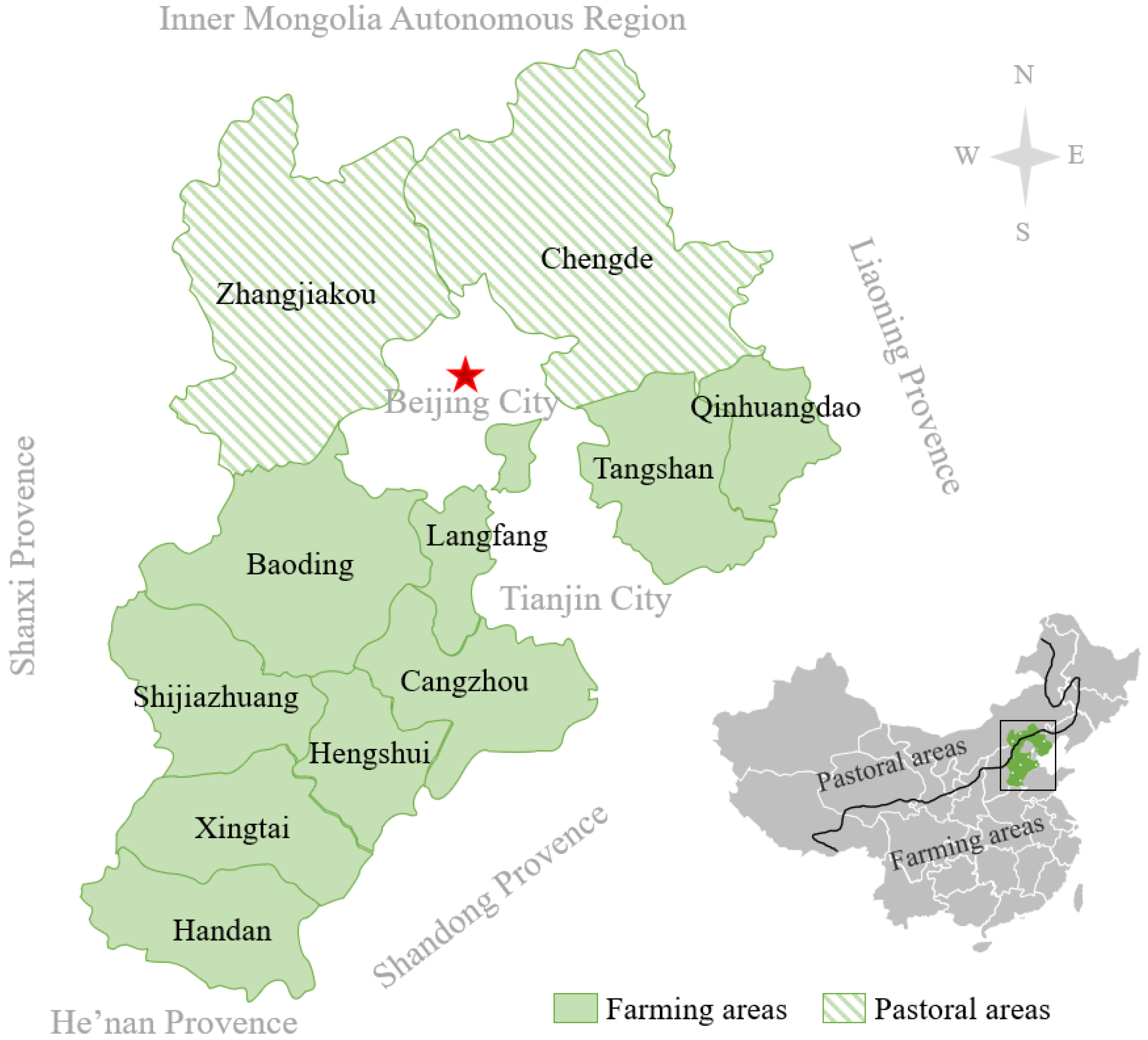
This study fills the gap by comparing different calf production systems based on an “in-farm”, on-field approach. The super-efficiency DEA model, with the undesirable outputs considered, was constructed after interviewing 218 farmers and 12 local county governments. The Tobit model was used to analyze the factors influencing different systems. The working hypotheses of the study are: (1) appropriate environmental regulation can encourage producers to improve the efficiency of beef cattle production; and (2) producers are not the “perfectly rational economic man”, as they are affected by their own knowledge and ability, as well as their soundings, so that the ability to obtain and process information is limited. The more knowledge one has, the higher one’s level of rationality is.

2. Materials and Methods

2.1. The Modeling Approach

To investigate the technical efficiency of different beef calf production systems, our study consisted of two steps: (1) measuring the technical efficiency with undesirable outputs considered; and (2) evaluating the impacts of factors on technical efficiency.

2.1.1. Efficiency Measurement Model: Super-Efficiency DEA Model with Undesirable Outputs

DEA, a non-parametric technical efficiency system analytical method, is a comparative efficiency evaluation tool based on multi-input and multi-output objects that was proposed by Charnes et al. [21]. It is not a statistical analysis model but a linear programming model. As the natural laws of animal growth make it difficult to control input factors, this study adopts the output-oriented DEA model as the basic model. Tone constructed both an output-orientation super-efficiency DEA model and an undesirable output model [22,23]. Based on Cheng Gang’s findings, the two models built by Tone can be further developed into a super-efficiency DEA model with undesirable outputs considered, which has also been used in previous studies [24,25]. The model is as follows:
min φ = 1 + 1 m i = 1 m s i x i k 1 1 q 1 + q 2 r = 1 q 1 s r + y r k + t = 1 q 2 s t b b r k
s t .   j = 1 , j k n λ j x i j s i x i k ;
j = 1 , j k n λ j y r j + s r + y r k ;
j = 1 , j k n λ j y b t j s t b b t k ;
1 1 q 1 + q 2 r = 1 q 1 s r + y r k + t = 1 q 2 s t b b r k > 0 ;
λ j ,   s i ,   s r + ,   s t b 0 ;
i = 1 , 2 , 3 , m ; j = 1 , 2 , 3 , , n j k ;
r = 1 , 2 , 3 , , q 1 ; t = 1 , 2 , 3 , · · · · · · , q 2 .
where i is the number of input factors, j is the number of decision-making units (DMU), r is the number of desirable outputs, x i j is the input factor i of DMUj, y r j is the output r of DMUj, and m, q 1 and q 2 are the numbers of input factors, desirable outputs and undesirable outputs, respectively. Furthermore, s i , s r + and s t b are the input slack variable, desirable outputs and undesirable outputs, respectively, and λ j is the weight variable.
Moreover, φ is the minimum distance between the production state of the evaluated DMU and the production frontier formed by all DMUs. If φ < 1 , the DMU has an efficiency loss, and if φ 1 , the production is effective. The larger the φ value is, the higher the efficiency is. The objective function of the model min φ is to find the optimal solution φ * , that is, the technical efficiency (TE).
This model implies that the scale of production is constant, and the technical efficiency is calculated under the condition of constant return to scale (CRS-DEA). That is, all DMUs are assumed to reach the optimal production scale; thus, this technical efficiency includes scale efficiency. If the scale of production is variable—that is, the constraint equation j = 1 , j k n λ j = 1 is added to the model—a model with variable returns to scale (VRS-DEA) can be obtained. This model assumes that the DMU can adjust the production scale to achieve the optimal production efficiency, and the calculated technical efficiency excludes the influence of the scale. Thus, it is termed as pure technical efficiency (PTE). The relationship between the TE and PTE can also be used to calculate the scale efficiency (SE), SE = TE/PTE.

2.1.2. Evaluation Model of the Influencing Factors: Tobit Regression Model

For the discontinuous data and limited dependent variables, this study adopts the Tobit model to study how the influencing factors function, which are not included in the efficiency measurements, affecting the technical efficiency. After obtaining the production efficiency, the Tobit regression model was constructed with the efficiency as the dependent variable and influencing factors as the independent variables. The Tobit method has also often been used in previous studies on factors influencing production efficiency [16,26]. The Tobit model is as follows:
Y i = α i + β X i + ε ,   α i + β X i + ε > 0   0 ,   α i + β X i + ε 0
where X i is the explanatory variable, representing the factors influencing efficiency; Y i is explained variable, that is, the production efficiency; β is the regression coefficient; and ε is the random interference term, ε ~ N 0 , σ 2 .

2.2. Beef Cattle Production in China

At present, the most widely distributed beef cattle breed in China is the Simmental cattle breed (crossbred with Chinese indigenous breeds), with some cattle being placed in confinement, some grazing and some semi-grazing (grazing in daytime but confined at night) [2]. In addition, there are also many Holstein bulls placed in confinement in farming areas, which is an important part of beef cattle farming in China [27,28]. Due to the impacts of ecological and environmental protection policies, grazing has been restricted or even banned in many areas of China. Grazing is only allowed during a specified period of time per day in a specified season, and for the rest of the time, cattle must be kept in confinement. The extensive production system (grazing) has been limited to a very small area facing current ecological protection policies in China and is not worth studying. Beef cattle production can be divided into two stages: the calf production period and the cattle fattening period. The calf production period is the stage from the calf’s birth to about 6 months old (with a weight of about 250 kg), while fattening is the stage from the end of calf production to the adult cattle being sent to the slaughterhouse. Due to the differences in growth laws, the nutritional requirements and feeding management priorities of these two stages are quite different, and calf production is the start of the beef cattle industry. Therefore, this study focuses on the main three beef calf production systems. Referring to “Terrestrial Animal Health Standards Commission Report”, we have named them as follows:
(1)
Simmental calf intensive production system (CIPS): after birth, the Simmental calves are placed in confinement. Calves depend on daily animal husbandry for the provision of food, shelter and water. Calves are kept together with cows at birth to facilitate lactation and are kept separately after weaning.
(2)
Simmental calf semi-intensive production system (SCIPS): unlike CIPS, these calves have the opportunity to graze in a wide range of natural outdoor settings during the designated period (usually from 1 May to 1 October every year, from 8 AM to 8 PM every day), foraging freely, and are confined for the rest of the time.
(3)
Holstein bull calf intensive production system (BCIPS): this system is not for breeding but for meat. As in the case of CIPS, after birth the calves are placed in confinement, depending on daily animal husbandry for the provision of food, shelter and water. However, unlike CIPS, the breed of BCIPS is Holstein cattle instead of Simmental cattle, and the calves are fed separately from cows after birth and are bottle-fed instead of being suckled by cows. BCIPS has little in common with CIPS.

2.2.1. Variable Selection for Empirical Specification

Beef cattle production is based on the law of animal growth, and the living habits of beef cattle limit the range of input and output variables and influencing factor variables. In studies of this kind, herd size, feeds, veterinary costs, fixed costs, labor costs, etc., are usually included as inputs [15,29,30]. The value-added or physical weights of cattle have been used as outputs in previous studies [31,32]. This research included the feed, labor and infrastructure construction as input variables, and took the cattle weight gain as an output. At the same time, this paper considers the high-quality development of the industry, and carbon emissions and pollution emissions are considered as the main environmental problems in the development of the beef cattle industry. Therefore, referring to the literature on agricultural green production efficiency, carbon and pollutant emissions are listed as undesired outputs of beef cattle production [15]. The variables used in this article are described in detail below.
The input variables include basic production costs (BPC), forage (including roughage (RH) and concentrated feed (CF)), labor (LB) and other apportioned expenses (AE). The feedstock is allocated according to the nutritional needs of beef cattle at different stages of growth. In this study, the forages of cow and calves were calculated separately. Cow forage was defined as the weight and cost of feed from the breeding to the weaning of calves. The average daily feed is the weight and cost of each calf from birth to market. The material inputs of beef cattle production vary greatly under different production systems. To facilitate the construction of a common production frontier, the production costs of CIPS and BCIPS are calculated as follows: the production cycle costs of CIPS (including forage cost, birth cost, labor cost and material allocation) are combined as the BPC, while the costs of buying a newborn calf and milk in BCIPS are combined as the BPC. The other apportioned expenses (AE) include asset depreciation, medical and epidemic prevention expenses, water, electricity and fuel expenses, repair expenses and other expenses, which are not counted separately. In addition, the production cycle cost, as defined here, is the production cost of single animal in the same herd of beef cattle on the whole farm of the farmers who responded to the interview questionnaire, including the labor, forage, material inputs and other aspects. It is important to note that the cycle cost, here, includes the loss due to the death of calves on the farm. For example, if a farm raises 30 calves in the same herd, and 1 cow dies unexpectedly in the feeding process, and only 29 cows are normally sold, then the production cycle cost of each cow is the share of the total production cost (from buying to being sold or dying) of 30 calves versus 29 beef cattle.
Beef cattle production not only produces calves, but also produces air and water pollution. In this study, the weight gain of the calves (WG) was taken as the desired output, that is, the total weight gain of the calves from birth to market. As for BCIPS, the weight gain refers to the weight of the calves from birth to slaughter. Carbon emissions (CE) and pollutant production (PP) were selected as the undesirable outputs. The pollutants produced in beef cattle farming mainly include COD, TN (total nitrogen), TP (total phosphorus), copper and zinc, etc. These pollutants are mainly produced from dung and urine. Carbon emissions are a shorthand for greenhouse gas emissions. The main greenhouse gases are CO2, CH4 and N2O. In the accounting convention for carbon emissions, the CO2 of livestock and poultry is assumed to be 0, because it is mainly produced by the respiration of livestock, which is a basic demand for animal survival. The CH4 and N2O are the main carbon emissions of beef cattle production. N2O is mainly produced by fecal and urine excreta, while CH4 is mainly produced by beef cattle gastrointestinal fermentation in addition to fecal and urine excreta. To ensure the consistency and comparability of the three production systems, only the carbon emissions and pollutant production of the calves were considered in this study, and the undesired output of the cows was not considered. The IPCC (Intergovernmental Panel on Climate Change) regularly publishes CH4 emissions from various industries around the world, and China’s N2O emissions from livestock and poultry have also been published in the FAO (Food and Agriculture Organization of the United Nations) report, but they are not applicable to our research [5,27]. In this paper, according to the growth characteristics of beef cattle, carbon emission and pollutant production coefficients were calculated by referring to the calculation method in the “Manual of Emission Coefficients and Emission Coefficients of Livestock and Poultry Production in the National Pollution Source Census” (MECLPSC), the IPCC carbon emission coefficient method and the FAO report (the specific calculation formula is in Appendix A), as shown in Table 1.
Beef cattle production is affected by livestock managers and farms, as well as social surroundings. Therefore, the individual characteristics of farms and farmers, industrial environment, policies and social surroundings are selected as the main categories of the influencing factors in the study. Individual characteristics include six variables: the farmer’s educational level (EL), age (AGE), political or social role (PR), management level (ML) and years of professional production (YP) experience, and the size of the farm (S). The industrial environment includes three variables: the source of corn (including silage corn) (SC), source of dairy bull calves (SB) and the number of dominant competitors of other livestock and poultry production (sheep, pigs, and poultry) (DC). The policy and social surroundings include five variables: whether the beef cattle industry is a local agricultural industry (MD), whether the farmers have received government subsidies (GS), whether government environmental and ecological policy has a real effect on production (PF), whether the farmers participate in cooperative organization (CO) and whether they participate in professional and technical training (TT).

2.2.2. Survey and Data Description

Selecting representative survey areas and conducting interviews were an important part of the survey. Hebei Province, in the north of China, has both farming and pastoral areas, being rich in beef cattle production varieties and modes, and is an important beef cattle industry province. According to the “China Agricultural and Rural Statistical Yearbook”, in 2020, the number of slaughtered beef cattle in Hebei Province was 3.35 million, and the beef output was 0.56 million tons, accounting for 7.34% and 8.26% of the national output, respectively. Furthermore, many beef cattle trading markets (such as the Zhangsanying market in Longhua, and the Qipanshan market in Weichang County) have been formed as part of the long-term industrial development of the country. Hebei, which plays an important role in China, is a typical and representative area of calf production. Calves are supplied to other regions with developed beef fattening industries, such as Henan, Shandong and Jiangsu in this case. Figure 1 shows the surveyed areas.
According to the variables and the characteristics of the survey areas, the research group designed a questionnaire and conducted interviews. From May to September 2021, we visited 218 beef calf production farms in 12 counties and districts (evenly distributed over farming and pastoral areas) and conducted 218 face-to-face interviews. Table A1 shows the number of valid samples from the counties, and the reader can refer to Appendix B. We also interviewed members of 12 counties and township governments in the form of discussions and obtained 12 samples. Beef calf production in these areas can represent the situation of Hebei and that of the country. Table 2 lists the variables used in the empirical analysis, including units of measurement. There were five input variables (BPC, CF, RH, LB, AE), one desirable output variable (WG), two undesirable output variables (PP, CE) and three influencing variables: (1) the characteristics of farms and farmers (AGE, PL, YP, PR, S, ML), (2) industrial environments (SC, SB, DC) and (3) the policy and social surroundings (MD, GS, PE, TT, CO) of the three production systems. Table 2 shows the standard deviations and the means of the variables.

3. Results

3.1. Analysis of the Results of the DEA Model

3.1.1. Technical Efficiency

We conducted an outlier test on the data before the DEA modeling, and the results show that the data are suitable for efficiency measurements. The reader should refer to Appendix C. Using the survey data of the input, desirable output, and undesirable output variables obtained from the survey, we obtained the values of the technical efficiency of beef calf production by different systems using the CRS-DEA model. Table 3 shows the TE of the different systems.
Overall, from the perspective of distribution, there is great variation among the systems. The minimum value of the TE of the sample population is 0.3778, the maximum value is 1.3071 and the mean value is 0.7084. A total of 56 (25.74%) of the samples fell into the range of 0.7, 0.8, and 15 (6.9%) of the samples fell into [1.0), all of which were not from BCIPS. The TE of BCIPS was relatively low, with all of the values being below 0.8.
The TE of SCIPS was the highest, with an average of 0.8001, and six samples had an efficiency value above 1.0, accounting for 11.5%. There are two reasons for this. On the one hand, the SCIPS takes advantage of free pasture resources during grazing (treated as zero, because it cannot be accounted for), so that the feed input of both cows and calves is lower than that of other production systems, which ultimately leads to a low BPC, as well as a low input of the CF and RH for the calves. On the other hand, grazing is the traditional production system of small- and medium-sized family farmers, with less material input in terms of the enclosure and other aspects.
The average TE of CIPS was 0.7729, which was higher than that of BCIPS but slightly lower than that of SCIPS. There were 36 samples that fell in the range of [0.7, 0.8), accounting for 33% of the total, and more than half of the samples fell in the range of [0.6, 0.8). On the one hand, all the input factors of CIPS were accurately accounted for. On the other hand, CIPS does not have the environmental advantages of grazing that benefit SCIPS. These are the main reasons for the difference in the TE between CIPS and SCIPS.
The TE of BCIPS was the lowest, with an average efficiency of 0.4999, while more than half of the samples were lower than 0.5, and more than 91.3% of the samples fell into the range of [0.4, 0.6]. This may be due to the breed and production systems. Firstly, because of breed-related reasons, the RH and CF demands of Holstein bull calves are greater than those of the Simmental calf during production, but the growth rate is slower, and longer growth cycles mean a higher CE and PP, which means more inputs but also fewer desirable outputs and more undesirable outputs for dairy bull breeding. Secondly, the BCIPS is a bottle feeding system, which requires artificial feeding (pumps), resulting in more LB.

3.1.2. Pure Technological Efficiency and Scale Efficiency

Consistent with the previous analysis, we obtained the values of the pure technical efficiency of beef calf production by the different systems using the VRS-DEA model. The SE is calculated using the relationship between TE and PTE. Table 4 shows the PTE and SE of different beef calf production systems.
From the efficiency distribution of the samples, we can see that the PTE and SE of the three production systems basically follow normal distributions. The peak of PTE falls in the range of [0.7, 0.8), with an average of 0.8367, while the peak of SE falls in [0.8, 0.9), with an average of 0.8359. The PTE and SE of BCIPS are distributed in the lower efficiency interval; the distributions of the PTE and SE of crossbred cattle production are higher than those of BCIPS; and the PTE of crossbred cattle reared in captivity is slightly lower than that of the cattle reared in SCIPS, but the SE is slightly higher.
SCIPS produced the maximum PTE (1.5723) and SE (1.2255), while BCIPS produced both the minimum PTE and SE. This shows that great efficiency is lost in regard to the PTE of BCIPS compared with Simmental calf production systems. The loss of PTE is slightly larger in the CIPS, whereas the loss of SE is relatively serious in the SCIPS. The sample distribution peaks of the PTE and SE of BCIPS are concentrated in the range of [0.6, 0.7), and the concentration degree of pure PTE is slightly higher, with 31 samples falling in the range of [0.6, 0.7), accounting for 54% of the total, while the sample size of the SE falling within this area is 23, accounting for 40% of the total. The mean values of the PTE and SE of dairy bull are lower than those of Simmental cattle. However, from the perspective of efficiency improvement, the maximum values of the PTE and SE of BCIPS are 0.6949 and 0.7211, respectively, which are both higher than the mean values of the other systems. There is room to improve the efficiency of BCIPS by optimizing the resource allocation and scale.

3.2. Results of the Analysis of the Tobit Regression

3.2.1. The Hypothesis Testing

The next important task was to take the TE, PTE and SE as the dependent variables individually and the influencing factors as the independent variables in order to build Tobit models for the regression analysis. The likelihood ratio test (LR) was performed on the data before the Tobit model regression analysis:
  • For the null hypothesis: H 0 : β = β 0
  • For the LR statistics: L R = 2 l n L r l n L u ~ χ 2 j
where L r is the likelihood function value estimated by constrained M L , and   L u is the likelihood function value obtained by unconstrained M L . If H 0 is correct, l n L r l n L u should be small. Table 5 shows the test results of the three models.
According to the test results above, the data of all the production systems reject the null hypothesis at a value of less than 1% (p < 0.01), indicating that the Tobit model is suitable for the regression analysis of factors affecting the efficiencies of the three production systems.

3.2.2. Estimation Results of the Factors Influencing the TE

In this section, the TEs of the three production systems are taken as the dependent variables, and the influencing factors are taken as the independent variables in order to construct the Tobit models individually for the regression estimations. The results are shown in Table 6. At the same time, we carry out a data fitting analysis, and the results (in Appendix D) show that the Tobit models constructed in this study are appropriate.
  • Individual characteristics of the farms and farmers
The TE of SCIPS was significantly positively affected by the ML at 1% and EL at 10%, and negatively affected by the YP at 1%. The ML and S had significant positive effects on the BCIPS at 1% and 10%. The SCIPS samples are mainly from pastoral areas. The higher the number of beef calf production years is, the greater the influence of traditional habits will be, and the lower the farmers’ degree of acceptance of new management methods and concepts will be. This may be the reason for the significant negative impact of the number of production years on the production efficiency at the 1% level. SCIPS is a system transformed from a grazing system, and the difference in the ML has a more obvious impact on the efficiency, while the manual feeding of Holstein bull calves requires better professional breeding management. However, for CIPS, the ML difference between farms is small, leading to its insignificant effect on the TE. Furthermore, none of the individual characteristics had a significant effect on CIPS.
2.
Industrial environment
The SC had a significant positive effect on both SCIPS and BCIPS. This is because the crops in pastoral areas are only ripe once per year, resulting in low yields of crops such as corn and a lack of feed. Therefore, the SC has an important impact on beef cattle production in pastoral areas. However, due to breed-related reasons, the Holstein bull calf has high demands for CF and RH, and the distance from the feed source has a considerable impact on production. In addition, farmers choose production plans according to the convenience of the feed when making decisions, which may be why the SC has a significant positive impact on the TE. The DC has a significant negative effect on the TE of CIPS at the 5% level. More DC means higher competition for resources and greater production pressures, which may be why DC has a significant negative effect on the TE of systems in which animals are confined.
3.
Policy and social surroundings
The MD, PE and TT had positive effects on CIPS at different significance levels. Furthermore, CO and TT had significant positive effects on SCIPS and BCIPS. The beef cattle industry, as the main agricultural industry, leads to developmental advantages in the region, and the government and all sectors of society show a high degree of support for it, which may be why the MD has a significant effect on CIPS at the 10% level. Training can enable farmers to master more feeding techniques, medical and epidemic prevention techniques and more advanced management methods, which may explain the significant positive effect of the TT on CIPS at the 5% level and on BCIPS at the 1% level. In addition, the PF of CIPS has a significant positive influence at 1%. The government ban policy allows for four advantages: large-scale investments by operators; the acceleration of the rate of return on investments; more concern about the input and output efficiency of production; and, finally, more attention given to nutrition, management, and so on. For grazing areas with long distances and inconvenient collective activities between farms, communication between farmers in regard to production technology becomes more important, which may be why the CO has a 10% significant positive effect on the TE in SCIPS.

3.2.3. Estimation Results of the Factors Influencing the PTE

Table 7 shows the regression results of the factors influencing the PTE. The EViews 10 software package was used for the model regression.
  • Individual characteristics of farms and farmers
AGE has a significant positive effect (1%) in the case of CIPS and BCIPS, but the coefficients are small. The YP has significant negative effects on SCIPS and BCIPS at the 1% and 5% levels, respectively. This may be due to the difficulty involved in changing traditional farming practices in the short term, making it more difficult for farmers to accept new ideas. For example, grazing is a traditional mode of farming in pastoral areas, and the longer the length of time for which the managers follow grazing practices is, the more they tend to follow the same management philosophy of grazing after the stage of semi-captivity. It also takes time for SCIPS farmers to adapt to government environmental policies. The ML has a significant positive effect on both dairy bull calving (1%) and CIPS (10%). Both systems are production activities carried out through appropriate management with limited resources, and with high input and output requirements, which require elevated management skills.
2.
Industrial environment
The SC has a significant positive effect (5%) in the case of semi-captive and dairy bulls, while the SB has a significant positive effect (1%) on dairy bull calving. Corn (including silage corn) is a main feed crop in the north of Hebei, while the SCIPS is mainly employed in the pastoral area, where the yield of corn is very low. Therefore, the SC is an important factor. Moreover, BCIPS generates a great demand for corn, and the abundance of local corn affects the forage formula of Holstein bull calf breeders, thus having a great impact on the PTE. Holstein new-born bull calves are the starting point of BCIPS. Local new-born bull calves constitute a geographical advantage, and dairy farms can provide milk resources necessary for the early growth of calves. This may be why the SB has a significant effect on the PTE of BCIPS.
3.
Policy and social surroundings
The GE has a significant positive effect (1%) on CIPS and a significant negative effect (10%) on SCIPS. After grazing became regulated by the government, the grazing period became shorter and the input of feed material increased, which resulted in a decrease in the PTE. Additionally, the impacts of environmental policies on intensive rearing are mainly reflected in the relocation and reconstruction of farms caused by the restrictions on rearing in the region, but the renewal of enclosures improves the growing environments of cows and calves, so that the production system becomes more standardized and the resource use and allocation becomes more scientific and rational. The TT had a significant positive effect (1%) on the PTE of CIPS and was at the 5% level for the other production systems. Production technology training enables farmers to acquire more knowledge of animal husbandry and veterinary technology, which enables them to be more professional in terms of disease prevention and scientific feeding. The reduction in diseases and reasonable advances in nutrition can improve the growth rate of beef cattle, which is an important factor explaining how technical training (TT) can improve the PTE. The CO had a significant positive effect (5%) on CIPS. Cooperatives enable beef cattle farmers to exchange production technology and knowledge and provide mutual support in production. Moreover, as cooperatives, they can enjoy many industrial support policies, which helps to improve PTE in CIPS.

3.2.4. Estimation Results of the Factors Influencing the SE

Table 8 shows the regression results of the Tobit models regarding factors influencing the SE. The EViews 10 software package was used for the model regression.
  • Individual characteristics of farms and farmers
ML had a significant positive effect (1%) on the SE of SCIPS. This finding means that the management level, in turn, improves the SE, that is, the improvement in their own technical level and management ability and the resource allocation efficiency of the production management. Other influencing factors were either insignificant or had small coefficients.
2.
Industrial environment
The SC had a significant positive effect (5%) on the SE of SCIPS. This is due to the lack of corn in pastoral areas, indicating that the greater the local corn supply is, the more favorable it is to increase the production scale so that it is close to optimal. The DC had a significant positive effect (1%) on CIPS. This result means that the increase in the number of competitors will reduce the SE of CIPS; that is, the more competitors there are, the less opportunity there is to approach the optimal scale, which may be caused by limited resources, such as feed materials, labor forces and policy support in the region.
3.
Policy and social surroundings
The PE had positive effects on the SE of CIPS and BCIPS at the significance levels of 1% and 5%, respectively. Environmental regulations changed the production environment and status of farms, which also changed the scale of the farms and made factor allocation more achievable. The MD had a significant positive effect (5%) on the SE of CIPS. This means that the beef cattle industry, as the main local agricultural industry, is more conducive to the improvement of the SE. In other words, beef cattle farms in regions with a beef cattle industry are the main agricultural industry and have a better scale and resource allocation.

3.2.5. Comparison of the Efficiency of Different Production Systems

Overall, the efficiency of the SCIPS is more susceptible to the effects of the individual characteristics of farms and farmers and the industrial environment, while the CIPS and BCIPS are more susceptible to the effects of policy and social surroundings. Specifically, the PE showed significant positive effects on the TE, PTE and SE of CIPS. Except for the negative effect of the PTE at 10%, the other effects on the efficiency of SCIPS were not significant. The effect of the PE on the SE was positive at the significance level of 5%, but the correlation coefficient was smaller than that of BCIPS. For SCIPS, the YP and SC showed significant effects on the TE, PTE and SE to different degrees. The individual efficiency value of BCIPS was also affected to a certain extent, while none of the efficiency values of CIPS were significantly affected by these two factors. The TE, PTE, and SE of BCIPS were all affected by the TT at different levels of significance, which is an important aspect that distinguishes it from the other production systems.

4. Discussion

The sustainable development of animal husbandry is important for meeting the increasing demand for animal food and the increasing pressure on the ecological environment. At present, no studies have examined the ecological and environmental problems of beef calf production. Moreover, its cycle is long (usually more than 20 months), and there are many production systems. However, the differences in technical efficiency and influencing factors at different stages and in different systems are still unclear. This study aims to address these areas.
In this study, we measured technological efficiency and evaluated impactful factors. The results show that the technical efficiency of different production systems varies greatly. Moreover, the effects of the environmental regulation of beef calf production in China differ between modes. The results of the empirical study support the hypothesis. That is, reasonable environmental regulation can force farmers to improve their production efficiency, thus helping to improve the production efficiency of beef cattle, provided that policies are adapted to the characteristics of local production systems. Producers are not completely rationality, and the more knowledge they have, the more productive they will be, provided that “knowledge” is adapted to production needs [33,34,35].
The results show differences in efficiency among beef calf production systems. The differences in the effective efficiency are, firstly, caused by the differences between the production systems themselves. The results showed that the distribution of the TE, PTE and SE of CIPS, SCIPS and BCIPS basically conform to the normal distribution. The TE of CIPS is significantly higher than that of BCIPS but lower than that of SCIPS. The PTE and SE of BCIPS are lower than those of CIPS. The SE of CIPS is higher than that of SCIPS, but their PTEs are almost the same. Since the whole process of CIPS is carried out in cattle pens, the calf number is larger than that of SCIPS. It has the highest level of industrialization and specialization, which is the main reason for the higher SE. However, because of the deterioration of the growth environment of beef cattle due to density, the calves reared in CIPS have no opportunity for free grazing, as in the SCIPS, and animal welfare is relatively poor. Meanwhile, a high density causes an increase in production costs, which is an important reason for the lower TE of CIPS compared to that of SCIPS. BCIPS has always been carried out in agricultural areas of China. As the animals reared in these systems are the offspring of Holstein cattle, rather than Simmental cattle, their growth rate is slower, while the feed input is larger, which is the main reason why the TE, PTE and SE are significantly lower than the values of the other production systems.
The results also show that some of the factors related to the individual characteristics of farms and farmers have significant positive effects, while others have no effect or even negative effects. Producers are not completely rational, and the more knowledge they have, the more productive they are. However, only useful and timely information can be called knowledge, and out-of-date information does not belong in the category of “knowledge” [36]. The ML represents modern specialized production knowledge, which has a positive effect on production efficiency, while the YP and AGE reflect traditional ideas and production experience to a certain extent. After industrial upgrading, their role will be reduced or even become a hindrance. Thus, the fact that the ML and YP have opposite effects on technical efficiency is not contradictory. In the case of SCIPS, the environmental regulations have changed their production systems, which means that the YP actually reflects the influence of the traditional grazing production system, while the ML represents the experience and management ability of SCIPS producers. The influence of the management level and experience on agriculture has been examined in previous studies [17,37]. The YP has a significant negative effect on the technical efficiency of SCIPS, although the coefficient is small. However, the ML has a significant positive effect on the technical efficiency of SCIPS. This is consistent with the impact of the government regulations mentioned above. Due to the government environmental regulations, in recent years, the grazing mode, which is, in fact, the extensive production mode, has been converted to a semi-intensive production mode. The more YP a farmer has, the more difficult it is for them to transition. The farmers’ attitudes and habits do not tend to change swiftly, which has an important impact on their technical efficiency [38,39]. This finding is in line with previous studies. Moreover, in semi-captive farming areas, most farmers have not developed mature and stable management experience, and there is a large disparity in the ML between farms, which is an important factor explaining why the ML has a significant positive effect on SCIPS.
We also studied the factors of the industrial environment. The SC is an important influencing factor, which had a significant positive effect on the TE, PTE and SE of SCIPS. Due to time constraints, the SCIPS has not formed into a perfect auxiliary industrial system, while the demand for corn increased significantly after the conversion from grazing to an intensive production system. Previous studies have also concluded that input factors (labors, feed, etc.) play a significant role in determining environmental technical efficiency [15]. At the same time, due to the existence of positive externalities, large farms will have a higher output per unit of input [16].
As shown by the results, the PE is one of the most significant factors in terms of policy and social surroundings. Appropriate environmental regulation can promote the improvement in the production efficiency. The PE has noticeable positive effects on the efficiencies of CIPS and BCIPS. Environmental regulations can potentially influence carbon emissions through improving technical efficiency [40], and they might enhance competitive advantages and obtain good economic benefits [19]. However, their influences on different production systems are not the same, which is indicated by the PTE-related effects of the PE on SCIPS and CIPS. CIPS and BCIPS are mainly distributed in agricultural areas, while SCIPS is mainly distributed in pastoral and semi-pastoral areas. For the former, the government’s policy of banning grazing requires the farmers to move their herds far away from residential areas and water sources, which forces them to update their production facilities. The reconstruction of farms requires operators to rethink the scale of new enclosures, machinery and equipment investments and other aspects according to their production knowledge and with reference to the surrounding successful farms, which constitutes the process of production scale optimization. Farmers are more actively learning new farming and management techniques due to financial pressures caused by new farms, which is consistent with Porter’s environmental regulation hypothesis [19]. Moreover, from the perspective of animal welfare, the relocation and reconstruction of farms led by government polices creates a more professional, superior and suitable growing environment for beef cattle, which can result in higher output and returns [41,42]. Similar results have been obtained in previous studies; for example, pig farmers re-evaluate various factors and choose a production scale that is more suitable for them, so that farmers tend to gradually moderate the scale of the operation and achieve a higher technical efficiency [20]. However, in the latter case, the effect of the environmental regulation is mainly policies that prohibit or restrict grazing, which has changed the production tradition and systems of farms. In the process of transition from extensive production systems to semi- intensive production systems, most farms find it difficult to adapt due to many factors, such as extensive traditions and technology, and the use of free pasture resources is reduced due to the restrictions on regional cultivation, which is the main reason for the negative effect. This illustrates that the environmental regulation policy must adapt to the mode of production; an effective policy implementation must give full consideration to the desired effect and should not simply copy those applied in other places or other industrial modes [43]. Compared to the literature, our study is more expansive, as we compared different production systems and found that the same environmental regulation plays a different role in different production systems, and we explained this phenomenon.
In addition, the results also showed that the TT had a significant impact on the technical efficiency of CIPS and BCIPS, especially on the TE, PTE and SE of BCIPS. The results, showing that technical training has a significant positive effect on livestock production, have generally been verified [17,44]. The production process of BCIPS and CIPS is carried out in confinement, which is characterized by specialization and refinement. Intensive farming reduces animal welfare (for example, uncomfortable conditions make animals more susceptible to disease and slow growth), which requires improved technology. In particular, bottle feeding is essential for BCIPS, which requires artificial milk pump teats at the initial stage of calf admission, which is technically challenging. Accordingly, the ML has a significant positive impact on the technical efficiency of dairy bull calving.

5. Conclusions

This study reveals many phenomena that have not been elucidated before and explains them in detail. The effects of the same factors on the technical efficiency of different production systems can differ greatly. The characteristics of production systems determine the process and final effect of each influencing factor on the production efficiency. Appropriate environmental regulation has a positive effect on the improvement of the production efficiency of the CIPS. Reasonable policies can encourage beef cattle farmers towards modernization and the specialization of production. However, measures should be taken according to local conditions. Policies applicable to other industrial models or other regions may not be applicable to a given region. Producers are not completely rational. The more modern knowledge they have, the greater the benefits will be in terms of improving the production efficiency. However, for the beef cattle industry in China today, the process of industrial upgrading, especially the specialization and standardization of beef cattle production, means that production experience may not play a role, and in some cases, will hinder the process. Therefore, the real-time updating of professional technical training and management concept training plays an important role. In addition, the efficiency differences brought about by different breeds are evident, which are essential differences that cannot meaningfully be changed by external factors; thus, breed improvement is of great significance for the development of the beef cattle industry. This study considered all the factors involved in beef cattle production in both agricultural and pastoral areas, and the three models studied were representative. Thus, these findings are generally applicable and can be extended to other areas.
Due to COVID-19, although the scope and sample applied meet the requirements of statistics and econometrics, they are not extensive enough, and the results need to be verified further. We did not study the allocation efficiency and spatial efficiency in this paper, which are directions for further research. Future studies should also examine the effects of influencing factors, such as the offset effect on the efficiency of subsidy policies and regulation policies.

Author Contributions

Conceptualization, Y.X. and J.Y.; methodology, Y.X.; software, Y.C. and Y.X.; validation, J.Y. and C.M.; formal Analysis, Y.X. and J.Y.; investigation, Y.X., J.Y. and Y.Z.; resources, J.Y. and Y.Z.; data curation, H.Z. (Haijing Zheng); writing—original draft preparation, Y.X.; writing—review and editing, J.Y.; visualization, H.Z. (Haijing Zheng); supervision, project administration and funding acquisition, J.Y. and H.Z. (Huifeng Zhao). All authors have read and agreed to the published version of the manuscript.

Funding

This research was funded by the National Philosophy and Social Science Foundation of China, grant number 19CJY023, and the Modern Agricultural Industrial Technique System of Hebei Province: Industrial Economic Position of Innovation Teams Focusing on Beef Cattle, grant number HBCT2018130301.

Institutional Review Board Statement

Not applicable.

Informed Consent Statement

Not applicable.

Data Availability Statement

Not applicable.

Conflicts of Interest

The authors declare no conflict of interest.

Appendix A

Formula for estimating the coefficient of the pollutant:
F P F D s i t e = F P F D d e f a u l t × W s i t e 0.75 W d e f a u l t 0.75
where F P F D s i t e is the coefficient of the pollutant after conversion; F P F D d e f a u l t is the coefficient of the pollutant found in MECLPSC; W d e f a u l t is the weight of beef cattle in the corresponding area; and W s i t e is the weight obtained in the survey.
Formula for estimating the coefficient of carbon emissions ( C H 4 ):
C C H 4 s i t e = C H 4 d e f a u l t F N d e f a u l t × F U s i t e × W s i t e 0.75 W d e f a u l t 0.75
where C C H 4 s i t e is the coefficient of carbon emissions after conversion; C H 4 d e f a u l t is the coefficient of the pollutant found in the FAO report; F U d e f a u l t is the feces and urine excretion of beef cattle published in MECLPSC; W d e f a u l t is the weight of beef cattle in the corresponding area; and W s i t e is the weight obtained in the survey; F U s i t e is the feces and urine excretion of beef cattle in the survey area published in MECLPSC. The F U d e f a u l t and F U s i t e are from the Chinese Report, and F U d e f a u l t denotes the emissions corresponding to the area reported C H 4 d e f a u l t in the FAO report, while F U s i t e corresponds to the survey area.
Formula for estimating the coefficient of carbon emissions ( N 2 O ):
C N 2 O s i t e = N 2 O d e f a u l t F N d e f a u l t × F N s i t e × W s i t e 0.75 W d e f a u l t 0.75
where C N 2 O s i t e is the coefficient of carbon emissions after conversion; N 2 O d e f a u l t is the coefficient of the pollutant found in the IPCC report; F U d e f a u l t is the feces and urine excretion of beef cattle published in MECLPSC; W d e f a u l t is the weight of beef cattle in the corresponding area; W s i t e is the weight obtained in the survey; F U s i t e is the feces and urine excretion of beef cattle in the survey area published in MECLPSC. The F U d e f a u l t and F U s i t e are from the Chinese Report, and F U d e f a u l t denotes the emissions corresponding to the area reported N 2 O d e f a u l t in the IPCC report, while F U s i t e corresponds to the survey area.

Appendix B

Table A1. The Sample Volume from the Surveyed Counties.
CountyVolumeCountyVolume
Dingxing10Weichang9
Fengning10Xushui31
Longhua52Yixian14
Mancheng4Xingtang30
Qingyuan10Zhangbei14
Quyang3Yangquan3
Total
N = 218
CIPS109
SCIPS51
BCIPS58

Appendix C

Before calculating the efficiency, we took the logarithm of the data used and then conducted the singular value test using Eviews10. Figure A1 shows the test results.
Figure A1. Outlier Test Results of the Data Using the DEA Models.
Agriculture 12 01604 g0a1
Except for the PP values of several samples that fell close to the boundary, all the data were located within the range of the upper inner fence and the lower inner fence. After examining the questionnaires, all samples were confirmed to be correct and credible. Therefore, we believe that were no outliers, and all data are suitable for the efficiency analysis.

Appendix D

Data fit analysis of the Tobit models. According to the statistical principle, the smaller the AIC (Akaike info criterion), SC (Schwarz criterion) and HC (Hannan–Quinn criterion) values are, the better the degree of the fit of the Tobit model with the data will be. Table A2 shows the regression results and the AIC, SC and HC values.
Table A2. Results of the Data Fit Analysis of the Tobit Models.
VariablesIndependent VariablesCIPSSCIPSBCIPS
CoefficientZ StatisticCoefficientZ StatisticCoefficientZ Statistic
CConstant0.6229 ***2.839−1.0132−1.558−0.0342−0.234
Individual characteristics of farms and farmersAGE0.00241.493−0.0018−0.4170.00151.364
EL−0.0352−1.4330.1021 *1.648−0.0125−0.554
YB−0.0013−0.501−0.0157 ***−3.678−0.0073−1.112
PR−0.0150−0.536−0.0286−0.6280.08881.372
S0.00021.1140.00321.3940.0006 *1.700
ML0.12040.8001.6775 ***3.4580.4446 ***3.595
Industrial environmentSC0.01920.7550.1342 ***3.0790.0465 **2.474
SB----0.02451.448
DC−0.0610 **−2.353--−0.0157−0.692
Policy and social surroundingsMD0.0740 *1.843--0.03210.811
GS−0.0181−0.6640.02110.4190.02070.758
PE0.1640 ***6.056−0.0503−0.968−0.0114−0.617
TT0.0636 **1.9610.08141.4260.0609 ***2.824
CO0.02550.8660.0809 *1.681−0.0311−1.069
AIC−2.56851−1.11821−2.36162
SC−2.19814−0.72579−1.68813
HC−2.44831−0.93004−2.13874
* p ≤ 0.05, ** p ≤ 0.01, *** p ≤ 0.001.
After deleting insignificant influencing factors (AGE, PR, SB and GS), as shown in Table 6, the Tobit models were reconstructed. Table A3 shows the regression results of test models (1) and the AIC, SC and HC values.
Table A3. Test Results (1) of the Data Fit Analysis of the Tobit Models.
VariablesIndependent VariablesCIPSSCIPSBCIPS
CoefficientZ StatisticCoefficientZ StatisticCoefficientZ Statistic
CConstant0.5975 ***4.5740.9376 *1.7110.2802 *1.699
Individual characteristics of farms and farmersAGE------
EL−0.0234−1.569−0.06290.0450.01130.3924
YP0.00020.115−0.0093 **0.004−0.00820.008
PR------
S0.00011.442−0.00070.0020.00010.035
ML0.1961 **2.1460.14400.4410.4083 ***2.623
Industrial environmentSC0.0211.5540.04440.0410.0549 **2.293
SB------
DC−0.0108−0.699--−0.0213−1.261
Policy and social surroundingsMD0.0199−0.828--−0.0396−1.261
GS------
PE0.1084 ***6.4250.1082 **0.0500.01570.665
TT0.0672 ***3.3650.1313 **0.0520.02861.173
CO0.0265 *1.5140.0701 *0.041−0.0457−0.668
AIC−2.55733−1.02373−2.13205
SC−2.06104−0.64494−1.70193
HC−2.43717−1.07898−1.96489
* p ≤ 0.05, ** p ≤ 0.01, *** p ≤ 0.001.
The three variables of the SB, DC and MD were deleted (some of them do not play roles in certain production modes) and the Tobit regression was performed again. Table A4 shows the regression results of the test models (2) and AIC, SC and HC values.
Table A4. Test Results (2) of the Data Fit Analysis of the Tobit Models.
VariablesIndependent VariablesCIPSSCIPSBCIPS
CoefficientZ StatisticCoefficientZ StatisticCoefficientZ Statistic
CConstant0.4575 ***4.587−1.0132−1.5580.02610.151
Individual characteristics of farms and farmersAGE0.0026 ***2.681−0.0018−0.4170.0004 ***2.701
EL−0.0152−1.0680.1021 *1.6480.02010.747
YP0.0001−0.019−0.0157 ***−3.678−0.0151 **−1.985
PR−0.0061−0.361−0.0286−0.6280.0690.989
S0.00010.7780.00321.394−0.0001−0.459
ML0.1798 **2.2441.6775 ***3.4580.4543 ***3.172
Industrial environmentSC0.01761.1550.1342 ***3.0790.0221 ***2.585
SB------
DC------
Policy and social surroundingsMD------
GS−0.0058−0.3680.02110.419−0.0201−0.931
PE0.1095 ***6.728−0.0503−0.9680.03021.413
TT0.0628 ***3.2560.08141.4260.0520 **2.099
CO0.0280 *1.6570.0809 *1.681−0.0396−1.171
AIC−2.51821−1.11821−2.23792
SC−2.27722−0.72579−1.77196
HC−2.40804−0.93004−2.05683
* p ≤ 0.05, ** p ≤ 0.01, *** p ≤ 0.001.
As shown in the three tables above, at least two of the three information values (AIC, SC and HC) in Table A2 are smaller than the others. Thus, the fitting degree of the models shown in Table A2 is better than that of the others, and the Tobit models constructed in this study are relatively appropriate.

References

  1. Ahmed, S.; Downs, S.; Fanzo, J. Advancing an Integrative Framework to Evaluate Sustainability in National Dietary Guidelines. Front. Sustain. Food Syst. 2019, 3, 76. [Google Scholar] [CrossRef] [Green Version]
  2. CARS. Research on the Strategy of Sustainable Development of Modern Agricultural Industry in China: Beef Cattle and Yak Strategy Research Volume; China Agriculture Press: Beijing, China, 2016. [Google Scholar]
  3. Xue, Y.J.; Yan, J.L.; Zhao, H.F.; Ma, C.H. Meat Consumption Practice in China: An Empirical Analysis Based on Elastic Theory. J. Anim. Plant Sci. 2021, 31, 1779–1787. [Google Scholar] [CrossRef]
  4. Cao, B.; Zhang, Y.; Li, J.-Y.; Wang, Z.; Guo, A.-Z.; Liu, J.; Sun, B.-Z. Beef Cattle and Yak Industry Technology Development Report of 2021. Chin. J. Anim. Sci. 2022, 58, 245–250. [Google Scholar]
  5. Xue, Y.; Yan, J.; Zhao, H.; Zheng, H.; Ma, C. Can domestic animal husbandry develop independently? An empirical study of China’s beef cattle industry. Pak. J. Zool. 2022, 54, 1053–1062. [Google Scholar] [CrossRef]
  6. Svanbäck, A.; McCrackin, M.L.; Swaney, D.P.; Linefur, H.; Gustafsson, B.G.; Howarth, R.W.; Humborg, C. Reducing agricultural nutrient surpluses in a large catchment–Links to livestock density. Sci. Total Environ. 2019, 648, 1549–1559. [Google Scholar] [CrossRef]
  7. Martinez, J.; Dabert, P.; Barrington, S.; Burton, C. Livestock waste treatment systems for environmental quality, food safety, and sustainability. Bioresour. Technol. 2009, 100, 5527–5536. [Google Scholar] [CrossRef] [Green Version]
  8. Fawzy, S.; Osman, A.I.; Doran, J.; Rooney, D.W. Strategies for mitigation of climate change: A review. Environ. Chem. Lett. 2020, 18, 2069–2094. [Google Scholar] [CrossRef]
  9. Steinfeld, H.; Gerber, P.; Wassenaar, T.D.; Castel, V.; Rosales, M.; de Haan, C. Livestock’s Long Shadow: Environmental Issues and Options; Food and Agriculture Organization of the United Nations: Rome, Italy, 2006. [Google Scholar]
  10. IPCC. Mitigation of climate change. In Contribution of Working Group III to the Fifth Assessment Report of the Intergovernmental Panel on Climate Change; Intergovernmental Panel on Climate Change: Geneva, Switzerland, 2014; Volume 1454, p. 147. [Google Scholar]
  11. Metz, B.; Davidson, O.; Bosch, P.; Dave, R.; Meyer, L. Climate Change 2007-Mitigation of Climate Change; Intergovernmental Panel on Climate Change: Geneva, Switzerland, 2007. [Google Scholar]
  12. Qian, Y.; Song, K.; Hu, T.; Ying, T. Environmental status of livestock and poultry sectors in China under current transformation stage. Sci. Total Environ. 2018, 622, 702–709. [Google Scholar] [CrossRef]
  13. Li, P.; Shi, Z.; Wang, M. A review of research on pollution prevention and control of livestock manure discharge in China. Chin. J. Agric. Resour. Reg. Plan. 2020, 41, 37–44. [Google Scholar] [CrossRef]
  14. Streimikis, J.; Saraji, M.K. Green productivity and undesirable outputs in agriculture: A systematic review of DEA approach and policy recommendations. Econ. Res.-Ekon. Istraživanja 2021, 35, 819–853. [Google Scholar] [CrossRef]
  15. Haixiu, G.; Mingli, W.; Zizhong, S. Analysis on eco-efficiency and influencing factors of beef cattle in China. Chin. J. Agric. Resour. Reg. Plan. 2021, 42, 153–159. [Google Scholar]
  16. Shuai, S.; Fan, Z. Modeling the role of environmental regulations in regional green economy efficiency of China: Empirical evidence from super efficiency DEA-Tobit model. J. Environ. Manag. 2020, 261, 110227. [Google Scholar] [CrossRef] [PubMed]
  17. Wang, X. Research on Economic Efficiency of Mutton Sheep Production in China. Doctoral Thesis, China Agricultural University, Beijing, China, 2018. [Google Scholar]
  18. Khunchaikarn, S.; Mankeb, P.; Suwanmaneepong, S. Economic efficiency of beef cattle production in Thailand. J. Manag. Inf. Decis. Sci. 2020, 25, 1–9. [Google Scholar]
  19. Porter, M. America’s green strategy. Bus. Environ. A Read. 1996, 33, 1072. [Google Scholar]
  20. Yu, L. The Impact of Environmental Regulation on Green Total Factor Productivity of Pig Breeding Industry. Doctoral Thesis, Southwest University, Chongqing, China, 2020. [Google Scholar]
  21. Charnes, A.; Cooper, W.W.; Rhodes, E. Measuring the efficiency of decision making units. Eur. J. Oper. Res. 1978, 2, 429–444. [Google Scholar] [CrossRef]
  22. Cooper, W.W.; Seiford, L.M.; Tone, K. Data Envelopment Analysis: A Comprehensive Text with Models, Applications, References and DEA-Solver Software; Springer: New York, NY, USA, 2008. [Google Scholar]
  23. Tone, K. A slacks-based measure of super-efficiency in data envelopment analysis. Eur. J. Oper. Res. 2002, 143, 32–41. [Google Scholar] [CrossRef] [Green Version]
  24. Işgın, T.; Özel, R.; Bilgiç, A.; Florkowski, W.J.; Sevinç, M.R. DEA Performance Measurements in Cotton Production of Harran Plain, Turkey: A Single and Double Bootstrap Truncated Regression Approaches. Agriculture 2020, 10, 108. [Google Scholar] [CrossRef] [Green Version]
  25. Cheng, G. Date Envelopment Analysis: Methods and Maxdea Softwave; Intellectual Property Publishing House: Beijing, China, 2014. [Google Scholar]
  26. Tobin, J. Estimation of relationships for limited dependent variables. Econom. J. Econom. Soc. 1958, 26, 24–36. [Google Scholar] [CrossRef] [Green Version]
  27. Liu, G.K.; Yao, K.; Wang, S.; Zhao, L.; Zhang, X.; Guo, W.; Li, S.-L.; Wang, Y.; Wang, K. Progress in Holstein dairy calf fattening research. Heilongjiang Anim. Sci. Vet. Med. 2021, 5, 30–34. [Google Scholar] [CrossRef]
  28. Guo, Z.; Sun, F.; Ding, L.; Xin, H.; Wang, C.; Liu, L.; Zhao, X. Research Progress on the Production of Veal by Holstein Bull Calves. Technol. Advis. Anim. Husb. 2020, 2, 1–4. [Google Scholar]
  29. Otieno, D.J.; Hubbard, L.; Ruto, E. Technical efficiency and technology gaps in beef cattle production systems in Kenya: A stochastic metafrontier analysis. In Proceedings of the 85th Annual Conference of the Agricultural Economics Society (AES), Coventry, UK, 18–20 April 2011. [Google Scholar]
  30. Xue, Y.J.; Yan, J.L. Breeding efficiency of beef cattle in Chinese suitable areas. J. Anim. Plant Sci. 2019, 29, 1413–1423. [Google Scholar]
  31. Rakipova, A.N.; Gillespie, J.M.; Franke, D.E. Determinants of technical efficiency in Louisiana beef cattle production. J. ASFMRA 2003, 2003, 99–107. [Google Scholar]
  32. Featherstone, A.M.; Langemeier, M.R.; Ismet, M. A Nonparametric Analysis of Efficiency for a Sample of Kansas Beef Cow Farms. J. Agric. Appl. Econ. 1997, 29, 175–184. [Google Scholar] [CrossRef] [Green Version]
  33. Argote, L.; Miron-Spektor, E. Organizational learning: From experience to knowledge. Organ. Sci. 2011, 22, 1123–1137. [Google Scholar] [CrossRef] [Green Version]
  34. Paget, M.A. Experience and knowledge. Hum. Stud. 1983, 6, 67–90. [Google Scholar] [CrossRef]
  35. Simon, H.A. Bounded Rationality. In Utility and Probability; Springer: Berlin/Heidelberg, Germany, 1990; pp. 15–18. [Google Scholar]
  36. Fiori, S. Hayek’s theory on complexity and knowledge: Dichotomies, levels of analysis, and bounded rationality. J. Econ. Methodol. 2009, 16, 265–285. [Google Scholar] [CrossRef]
  37. Gusev, A.Y.; Koshkina, I.G. Labour productivity in the agricultural sector of the national economy is a key factor in the rise of production efficiency. In Proceedings of the IOP Conference Series: Earth and Environmental Science, NIT, Raipur, India, 25–26 February 2022; p. 012037. [Google Scholar]
  38. Pérez Urdiales, M.; Lansink, A.O.; Wall, A. Eco-efficiency Among Dairy Farmers: The Importance of Socio-economic Characteristics and Farmer Attitudes. Environ. Resour. Econ. 2016, 64, 559–574. [Google Scholar] [CrossRef]
  39. Huang, Y.; Luo, X.; Tang, L.; Yu, W. The power of habit: Does production experience lead to pesticide overuse? Environ. Sci. Pollut. Res. 2020, 27, 25287–25296. [Google Scholar] [CrossRef]
  40. Pei, Y.; Zhu, Y.; Liu, S.; Wang, X.; Cao, J. Environmental regulation and carbon emission: The mediation effect of technical efficiency. J. Clean. Prod. 2019, 236, 117599. [Google Scholar] [CrossRef]
  41. Cecchini, L.; Vieceli, L.; D’Urso, A.; Magistrali, C.F.; Forte, C.; Mignacca, S.A.; Trabalza-Marinucci, M.; Chiorri, M. Farm efficiency related to animal welfare performance and management of sheep farms in marginal areas of Central Italy: A two-stage DEA model. Ital. J. Anim. Sci. 2021, 20, 955–969. [Google Scholar] [CrossRef]
  42. Jo, H.; Nasrullah, M.; Jiang, B.; Li, X.; Bao, J. A survey of broiler farmers’ perceptions of animal welfare and their technical efficiency: A case study in northeast China. J. Appl. Anim. Welf. Sci. 2022, 25, 275–286. [Google Scholar] [CrossRef] [PubMed]
  43. Huang, Z. Guiding high-quality agricultural development with a new development philosophy. China Rural Work Newsl. 2021, 5, 38–40. [Google Scholar] [CrossRef]
  44. Wubeneh, N.; Ehui, S.K. Technical efficiency of smallholder dairy farmers in the central Ethiopian highlands. In Proceedings of the International Association of Agricultural Economists (IAAE), 2006 Annual Meeting, Queensland, Australia, 12–18 August 2006. [Google Scholar]
Figure 1. The Survey Farming Areas and Pastoral Areas.
Agriculture 12 01604 g001
Table 1. Coefficients of Pollutants and Carbon Emissions of Beef Calf Production in Different Survey Areas.
CattleRegionCoefficient of Pollutants a
(×10−3 kg·(per Head·per Year)−1)
Coefficient of Carbon Emissions a
(×10−3 kg CO2e·(per Head·per Year)−1) b
CH4N2OTotal
CalfSouth-central Hebei137.060461.07351.739662.8131
North Hebei184.686853.73881.530755.2695
Breeding CowSouth-central Hebei435.1783193.91355.5234199.4368
North Hebei586.3959170.62514.8600175.4851
a The coefficients are average values over a period of 300 kg of growth starting from 40 kg of body weight; b the unit kg CO2e is equivalent to 1 kg of CO2.
Table 2. Description of the Statistics for Variables Used in the Production Efficiency Analysis (Data from 218 Questionnaires).
VariablesVariable NameUnitsCIPSSCIPSBCIPS
MeanStd. DevMeanStd. DevMeanStd. Dev
Input variablesBPCyuan/head5965.10821.454128.30836.665004.65228.82
CFkg/head191.4153.80135.7378.69273.7365.22
RHkg/head140.7443.2597.0580.39312.1468.69
LBhours/head13.106.0213.675.6115.423.69
AEyuan/head21.8713.809.4910.1625.9012.84
Output variablesWGkg/head225.0820.16246.0360.71218.4325.97
PPkg/head30.984.5737.6110.6028.033.39
CEkg CO2e/head11.161.4211.413.2113.021.57
Individual characteristics of farms and farmersAGEAge46.166.4752.495.9045.287.98
ELPrimary or below = 1, Junior school = 2, High school = 3,
College or above = 4
2.140.481.790.562.140.35
YPYears7.204.7510.587.984.391.47
PRyes = 1, no = 00.170.370.280.450.020.13
SHead52.3895.4127.1513.8444.6737.01
ML0–21.200.101.220.061.070.07
Industrial environmentSClocal = 1, nonlocal = 00.460.500.620.480.560.50
SBlocal = 1, nonlocal = 0----0.460.50
DC 1.520.741.040.272.020.61
Policy and social surroundingsMDyes = 1, no = 00.830.381.000.000.390.49
GSyes = 1, no = 00.400.490.470.500.540.50
PEyes = 1, no = 00.500.500.680.470.490.50
TTyes = 1, no = 00.610.490.580.490.400.49
COyes = 1, no = 00.170.380.280.450.140.35
Note: BPC—basic production costs, RH—roughage, CF—concentrated feed, AE—other apportioned expenses, WG—the weight gain of the calf, CE—carbon emission, PP—pollutant production, AGE—age, EL—education level, YP—years of beef calf production, PR—political or social role, S—the size of the farm, ML—management level, SC—source of corn (including silage corn), SB—source of Holstein bull calves, MD—whether the beef cattle industry is the most important part of the local agricultural industry, DC—the number of dominant competitors of other livestock and poultry production, GS—whether government subsidies were received, PE—policy on the environment, whether government environmental and ecological policy has real effects on production, TT—participation in professional and technical training, CO—whether the farmers participate in cooperative organization.
Table 3. The Technical Efficiency (TE) of Different Beef Calf Production Systems Calculated by the CRS-DEA Model.
GroupTotalCIPSSCIPSBCIPS
[0.0, 0.4)2 (0.9%)002(3.5%)
[0.4, 0.5)31 (14.2%)2 (1.8%)029 (50.9%)
[0.5, 0.6)42 (19.3%)14 (12.8%)5 (9.6%)23 (40.4%)
[0.6, 0.7)28 (12.8%)19 (17.4%)7 (13.5%)2 (3.5%)
[0.7, 0.8)56 (25.7%)36 (33.0%)19 (36.5%)1 (1.8%)
[0.8, 0.9)27 (12.4%)17 (15.6%)10 (19.2%)0
[0.9, 1.0)17 (7.8%)12 (11.0%)5 (9.6%)0
[1.0, 1.1)5 (2.3%)4 (3.7%)1 (1.9%)0
[1.1, 1.2)7 (3.2%)3 (2.8%)4 (7.7%)0
[1.2, 2.0)3 (1.4%)2 (1.8%)1 (1.9%)0
Sample volume2181095257
Min.0.37780.48690.50080.3778
Max.1.30711.26001.30710.7319
Mean0.70840.77290.80010.4999
Table 4. The Pure Technical Efficiency (PTE) and Scale Efficiency (SE) of Different Beef Calf Production Systems Calculated by the VRS-DEA Model.
GroupsTotal SamplesCIPSSCIPSBCIPS
PTESEPTESEPTESEPTESE
[0.0, 0.4)00000000
[0.4, 0.5)10000010
[0.5, 0.6)22005022
[0.6, 0.7)382762723123
[0.7, 0.8)5651281319161722
[0.8, 0.9)54773958101059
[0.9, 1.0)4542243051111
[1.0, 1.1)131610311300
[1.1, 1.2)41214000
[1.2, 2.0)42021000
Min.0.49780.58900.65370.68740.62500.62700.49780.5890
Max.1.57231.22551.18581.22551.57231.00000.95650.9065
Mean0.83670.83590.86640.88510.93170.86470.69490.7211
Std. Dev0.14830.11640.11070.08870.16580.11620.07640.0745
Table 5. Hypothesis Test Results of the Tobit Model of Different Beef Calf Production Systems.
Title 1LR Statisticsp-ValueTest Results
SCIPS36.860.0001Null hypothesis is rejected
CIPS139.570.0001Null hypothesis is rejected
BCIPS28.700.0025Null hypothesis is rejected
Table 6. Estimation Results of the Factors Influencing the Technical Efficiency (TE) of Different Beef Calf Production Systems.
VariablesIndependent VariablesCIPSSCIPSBCIPS
CoefficientZ StatisticCoefficientZ StatisticCoefficientZ Statistic
CConstant0.6229 ***2.839−1.0132−1.558−0.0342−0.234
Individual characteristics of farms and farmersAGE0.00241.493−0.0018−0.4170.00151.364
EL−0.0352−1.4330.1021 *1.648−0.0125−0.554
YP−0.0013−0.501−0.0157 ***−3.678−0.0073−1.112
PR−0.0150−0.536−0.0286−0.6280.08881.372
S0.00021.1140.00321.3940.0006 *1.700
ML0.12040.8001.6775 ***3.4580.4446 ***3.595
Industrial environmentSC0.01920.7550.1342 ***3.0790.0465 **2.474
SB----0.02451.448
DC−0.0610 **−2.353--−0.0157−0.692
Policy and social surroundingsMD0.0740 *1.843--0.03210.811
GS−0.0181−0.6640.02110.4190.02070.758
PE0.1640 ***6.056−0.0503−0.968−0.0114−0.617
TT0.0636 **1.9610.08141.4260.0609 ***2.824
CO0.02550.8660.0809 *1.681−0.0311−1.069
Note: ***, ** and * mean significant at 1%, 5% and 10%, respectively. EViews 10 software package was used for the model regression.
Table 7. Estimation Results of the Factors Influencing the Pure Technical Efficiency (PTE) of Different Beef Calf Production Systems.
VariablesIndependent VariablesCIPSSCIPSBCIPS
CoefficientZ StatisticCoefficientZ StatisticCoefficientZ Statistic
CConstant0.5345 ***4.0100.79901.3890.07050.423
Individual characteristics of farms and farmersAGE0.0026 ***2.614−0.0003−0.0790.0034 ***2.714
EL−0.0180−1.206−0.0722−1.3160.01930.752
YP−0.0003−0.225−0.0110 ***−2.909−0.0156 **−2.094
PR−0.0065−0.380−0.0255−0.6340.09161.242
S0.00010.9570.00010.0620.00010.037
ML0.1517 *1.6590.24630.5740.4380 ***3.107
Industrial environmentSC0.01540.9990.0791 **2.0510.04779 **2.229
SB----0.0505 ***2.619
DC−0.0138−0.874--−0.0139−0.540
Policy and social surroundingsMD−0.0142−0.581--−0.0280−0.620
GS−0.0104−0.6270.02780.624−0.0177−0.568
PE0.1073 ***6.522−0.0832 *−1.8120.02461.165
TT0.0645 ***3.2740.1190 **2.3560.0483 **1.964
CO0.0330 **1.8400.08351.962−0.0371−1.120
Note: ***, ** and * mean significant at 1%, 5% and 10%, respectively.
Table 8. Estimation Results of the Factors Influencing the Scale Efficiency (SE) of Different Beef Calf Production Systems.
VariablesIndependent VariablesCIPSSCIPSBCIPS
CoefficientZ StatisticCoefficientZ StatisticCoefficientZ Statistic
CConstant0.9939 ***6.280−0.9140 *−1.8070.6073 ***3.696
Individual characteristics of farms and farmersAGE0.00010.063−0.0010−0.292−0.0014−1.141
EL−0.0163−0.920−0.0466−0.967−0.0392−1.547
YP−0.0012−0.678−0.0002 **−2.1740.00640.871
PR−0.0099−0.488−0.0022−0.0630.02730.375
S0.00010.5290.0036 **1.9970.0008 *1.897
ML0.01570.1441.5115 ***4.0060.17111.231
Industrial environmentSC0.00910.4970.0729 **2.1510.01640.776
SB----−0.0185−0.973
DC−0.0523 ***−2.801--−0.0039−0.154
Policy and social surroundingsMD0.0644 **2.225--−0.0054−0.121
GS−0.0090−0.457−0.0272−0.6960.04871.591
PE0.0718 ***3.6750.02820.6990.0408 **1.960
TT0.01360.582−0.0260−0.5860.0421 *1.736
CO−0.0005−0.0230.02130.569−0.0088−0.269
Note: ***, ** and * means significant at 1%, 5% and 10%, respectively.
Publisher’s Note: MDPI stays neutral with regard to jurisdictional claims in published maps and institutional affiliations.

