


Potential Impact of Future Climates on Rice Production in Ecuador Determined Using Kobayashi’s ‘Very Simple Model’

 , ,
, ,  , , , , and
Abstract
:1. Introduction
2. Materials and Methods
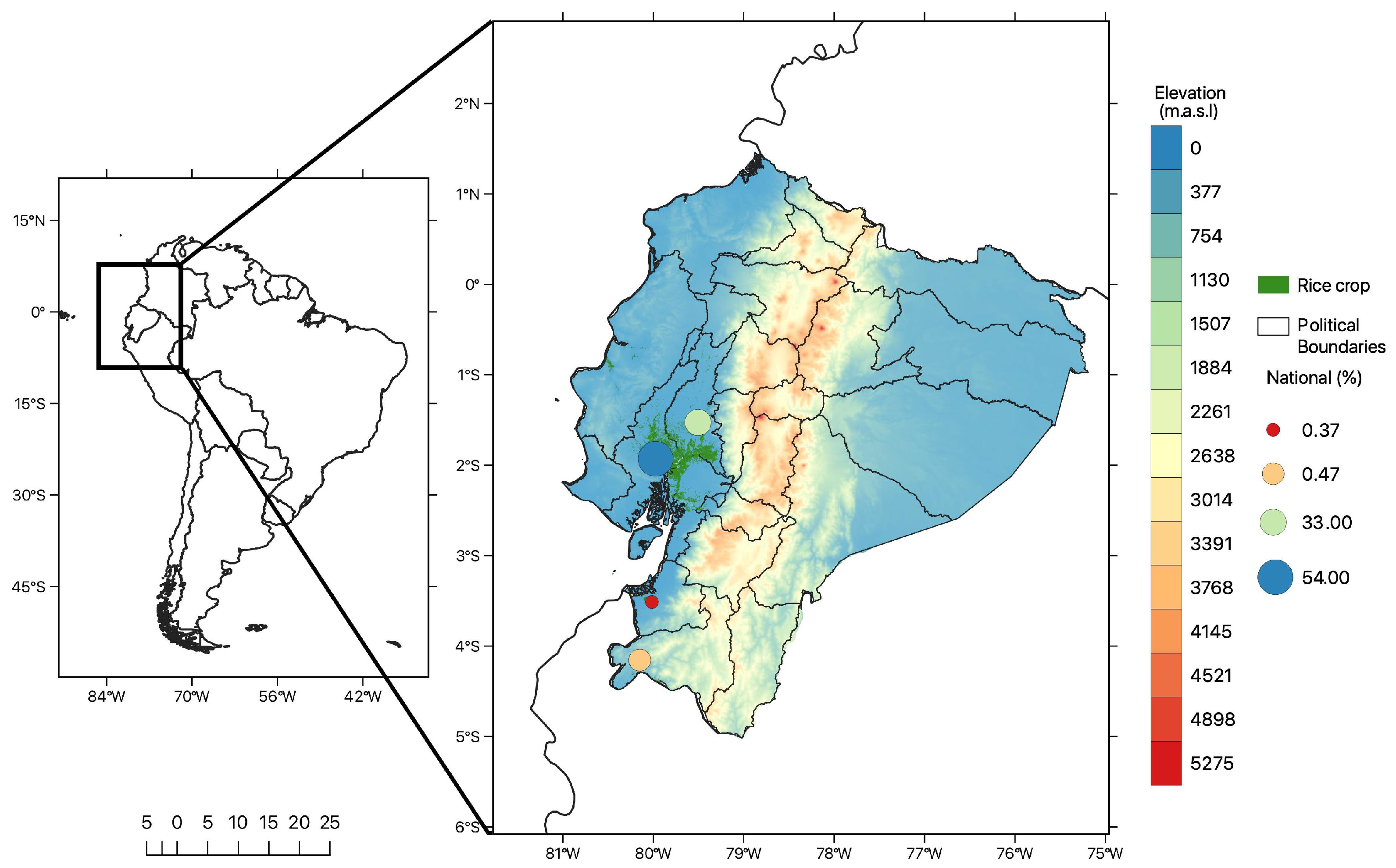
2.1. Study Area
2.2. Data and Methods
2.2.1. Description of the Very Simple Model (VSM)
2.2.2. Input Data Processing
2.2.3. Climate Change Impact Assessment
3. Results
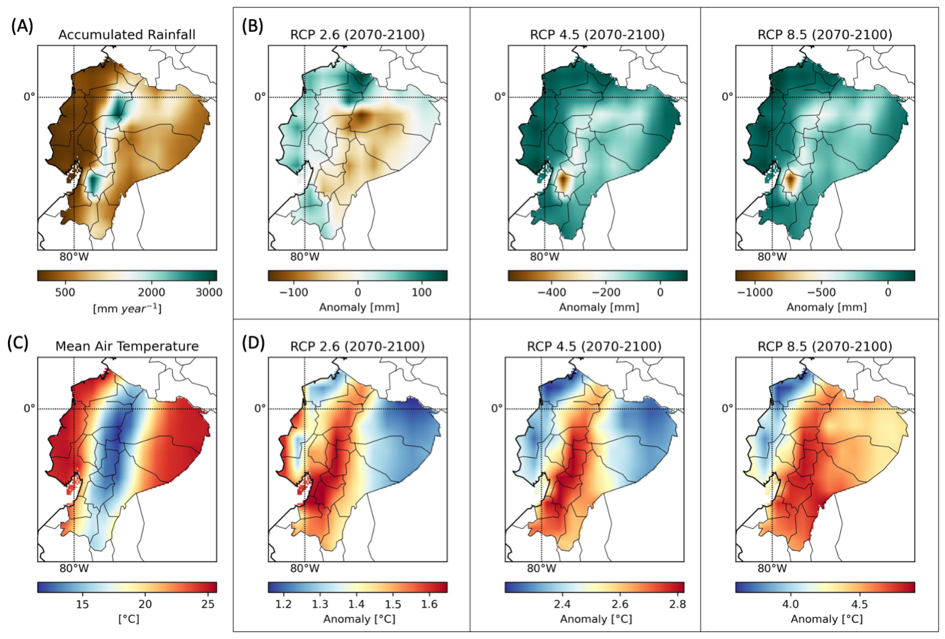
3.1. Projected Mean Change in Climatic Variables Based on RegCM4
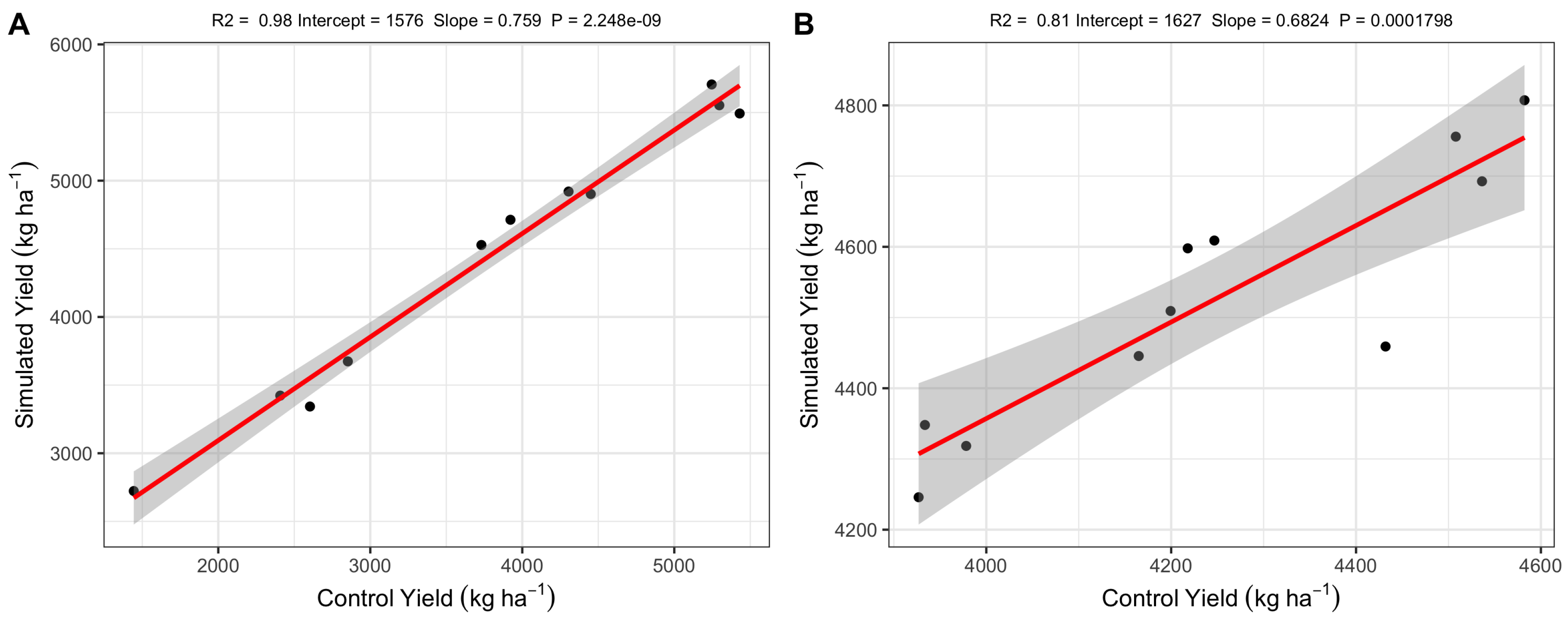
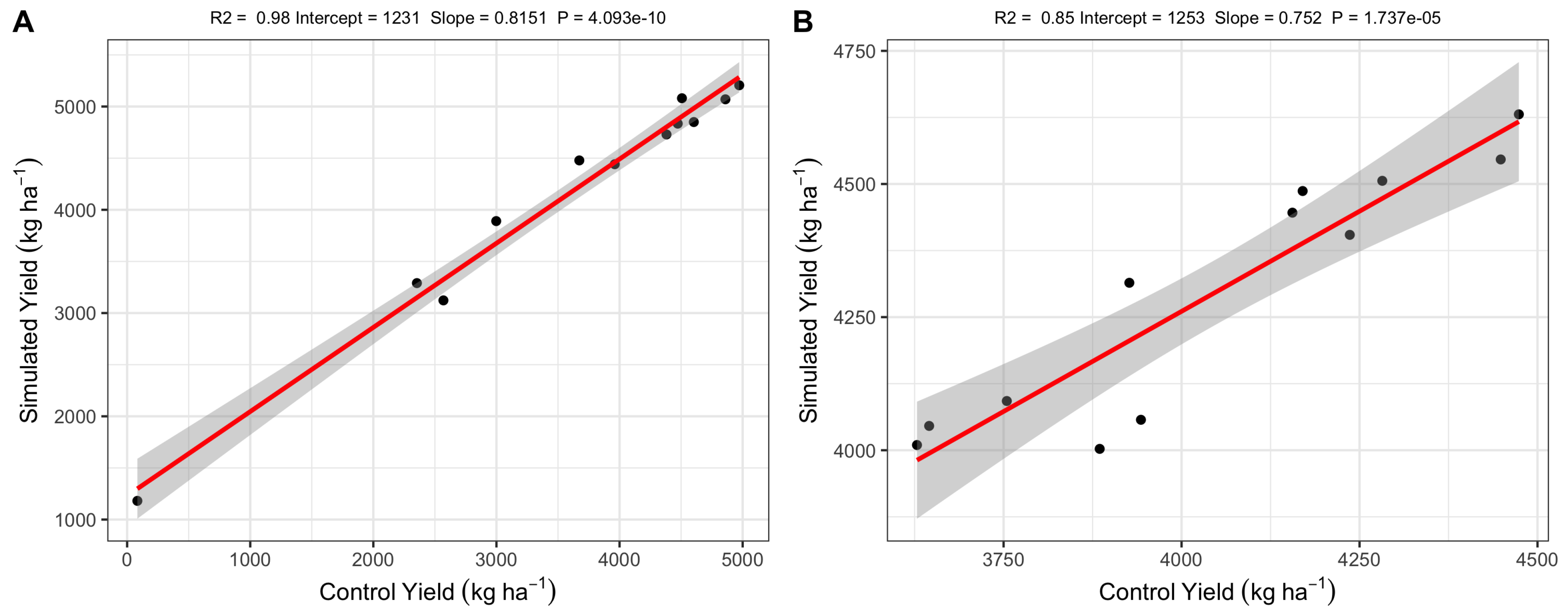
3.2. Model Suitability Confirmation
3.3. Model Results
4. Discussion
5. Conclusions
Supplementary Materials
Author Contributions
Funding
Institutional Review Board Statement
Informed Consent Statement
Data Availability Statement
Acknowledgments
Conflicts of Interest
Abbreviations
| HadGEM2-ES | Hadley Centre Global Environment Model version 2; |
| DSSAT | Decision Support System for Agrotechnology Transfer; |
| CORDEX | Coordinated Regional Climate 269 Downscaling Experiment; |
| RegCM4 | Regional Climate Modeling 141 System; |
| GDAL | Geospatial Data Abstraction Software Library; |
| NetCDF | Network Common Data Form; |
| IPCC | Intergovernmental Panel on Climate Change; |
| LULC | Land use and land cover; |
| SWAT | Soil and Water Assessment Tool; |
| RMSEn | Normalized root mean square error; |
| RMSE | Root mean square error; |
| VSM | Very simple model; |
| NCL | Research Command Language; |
| RCP | Representative concentration pathways; |
| GOF | Goodness-of-fit measures; |
| CO2 | Carbon dioxide; |
| MAE | Mean absolute error; |
| GCM | Global climate models; |
| RCM | Regional climate model; |
| LAI | Leaf area index; |
| RP | Reference period; |
| FP | Future period; |
| RH | Relative humidity. |
References
- Kong, W.; Zhong, H.; Gong, Z.; Fang, X.; Sun, T.; Deng, X.; Li, Y. Meta-analysis of salt stress transcriptome responses in different rice genotypes at the seedling stage. Plants 2019, 8, 64. [Google Scholar] [CrossRef] [PubMed] [Green Version]
- Yuan, S.; Peng, S.; Li, T. Evaluation and application of the ORYZA rice model under different crop managements with high-yielding rice cultivars in central China. Field Crops Res. 2017, 212, 115–125. [Google Scholar] [CrossRef]
- Seck, P.A.; Diagne, A.; Mohanty, S.; Wopereis, M. Crops that feed the world 7: Rice. Food Secur. 2012, 4, 7–24. [Google Scholar] [CrossRef]
- Godfray, H.C.J.; Beddington, J.R.; Crute, I.R.; Haddad, L.; Lawrence, D.; Muir, J.F.; Pretty, J.; Robinson, S.; Thomas, S.M.; Toulmin, C. Food Security: The Challenge of Feeding 9 Billion People. Science 2010, 327, 812–818. [Google Scholar] [CrossRef] [Green Version]
- Ullah, A.; Nawaz, A.; Farooq, M.; Siddique, K.H. Agricultural innovation and sustainable development: A case study of rice–wheat cropping systems in South Asia. Sustainability 2021, 13, 1965. [Google Scholar] [CrossRef]
- Sivakumar, M.V.; Gommes, R.; Baier, W. Agrometeorology and sustainable agriculture. Agric. For. Meteorol. 2000, 103, 11–26. [Google Scholar] [CrossRef]
- ESPAC. Encuesta de Superficie y Producción Agropecuaria Continua ESPAC 2017 Contenidos; INEC: Quito, Ecuador, 2017. [Google Scholar]
- Horgan, F.G.; Zhu, Q.; Portalanza, D.E.; Felix, M.I. Costs to Ecuador’s rice sector during the first decade of an apple snail invasion and policy recommendations for regions at risk. Crop Prot. 2021, 148, 105746. [Google Scholar] [CrossRef]
- INEC. Censo Nacional Agropecuario. 2019. Available online: https://www.ecuadorencifras.gob.ec/censo-nacional-agropecuario/ (accessed on 20 May 2021).
- FAO. Crops. 2017. License: CC BY-NC-SA 3.0 IGO. Available online: https://www.fao.org/faostat/en/#home (accessed on 20 May 2021).
- Alava, M.F.; Poaquiza, J.T.; Castillo, G.H. La producción arrocera del Ecuador. Rev. Espac. 2018, 39, 1–16. [Google Scholar]
- Marcelo, C. Rendimiento de Arroz en Cáscara, Primer Cuatrimestre 2017; Dirección de Análisis y Procesamiento de la Información Coordinación General del Sistema de Información Nacional Ministerio de Agricultura, Ganadería: Quito, Ecuador, 2017. [Google Scholar]
- Herrera-Fontana, M.E.; Chisaguano, A.M.; Villagomez, V.; Pozo, L.; Villar, M.; Castro, N.; Beltran, P. Food insecurity and malnutrition in vulnerable households with children under 5 years on the Ecuadorian coast: A post-earthquake analysis. Rural Remote Health 2020, 20, 5237. [Google Scholar] [CrossRef]
- Trisasongko, B.H.; Panuju, D.R.; Harimurti; Ramly, A.F.; Subroto, H. Rapid assessment of agriculture vulnerability to drought using GIS. Int. J. Technol. 2016, 7, 114–122. [Google Scholar] [CrossRef]
- Wang, J.; Wang, E.; Yang, X.; Zhang, F.; Yin, H. Increased yield potential of wheat-maize cropping system in the North China Plain by climate change adaptation. Clim. Chang. 2012, 113, 825–840. [Google Scholar] [CrossRef]
- Aryal, J.P.; Sapkota, T.B.; Khurana, R.; Khatri-Chhetri, A.; Rahut, D.B.; Jat, M.L. Climate change and agriculture in South Asia: Adaptation options in smallholder production systems. Environ. Dev. Sustain. 2020, 22, 5045–5075. [Google Scholar] [CrossRef] [Green Version]
- Huong, N.T.L.; Bo, Y.S.; Fahad, S. Economic impact of climate change on agriculture using Ricardian approach: A case of northwest Vietnam. J. Saudi Soc. Agric. Sci. 2019, 18, 449–457. [Google Scholar] [CrossRef]
- Yohannes, H. A Review on Relationship between Climate Change and Agriculture. J. Earth Sci. Clim. Chang. 2015, 7, 1–8. [Google Scholar] [CrossRef]
- IPCC. IPCC Fifth Assessment Synthesis Report-Climate Change 2014 Synthesis Report. In IPCC Fifth Assessment Synthesis Report-Climate Change 2014; Synthesis Report; IPCC: Geneva, Switzerland, 2014. [Google Scholar]
- IPCC. Summary for Policymakers. In Climate Change 2013—The Physical Science Basis; IPCC, Ed.; Cambridge University Press: Cambridge, UK, 2013; pp. 1–30. [Google Scholar] [CrossRef]
- Gupta, R.; Mishra, A. Climate change induced impact and uncertainty of rice yield of agro-ecological zones of India. Agric. Syst. 2019, 173, 1–11. [Google Scholar] [CrossRef]
- Muis, S.; Apecechea, M.I.; Dullaart, J.; de Lima Rego, J.; Madsen, K.S.; Su, J.; Yan, K.; Verlaan, M. A High-Resolution Global Dataset of Extreme Sea Levels, Tides, and Storm Surges, Including Future Projections. Front. Mar. Sci. 2020, 7, 263. [Google Scholar] [CrossRef]
- Sun, Q.; Miao, C.; Duan, Q.; Ashouri, H.; Sorooshian, S.; Hsu, K. A Review of Global Precipitation Data Sets: Data Sources, Estimation, and Intercomparisons. Rev. Geophys. 2018, 56, 79–107. [Google Scholar] [CrossRef] [Green Version]
- van Vuuren, D.P.; Edmonds, J.; Kainuma, M.; Riahi, K.; Thomson, A.; Hibbard, K.; Hurtt, G.C.; Kram, T.; Krey, V.; Lamarque, J.F.; et al. The representative concentration pathways: An overview. Clim. Chang. 2011, 109, 5–31. [Google Scholar] [CrossRef]
- Manzanas, R.; Gutiérrez, J.M.; Fernández, J.; van Meijgaard, E.; Calmanti, S.; Magariño, M.E.; Cofiño, A.S.; Herrera, S. Dynamical and statistical downscaling of seasonal temperature forecasts in Europe: Added value for user applications. Clim. Serv. 2018, 9, 44–56. [Google Scholar] [CrossRef]
- Maraun, D. Bias Correcting Climate Change Simulations—A Critical Review. Curr. Clim. Chang. Rep. 2016, 2, 211–220. [Google Scholar] [CrossRef]
- Amiri, E.; Razavipour, T.; Farid, A.; Bannayan, M. Effects of crop density and irrigation management on water productivity of rice production in northern Iran: Field and modeling approach. Commun. Soil Sci. Plant Anal. 2011, 42, 2085–2099. [Google Scholar] [CrossRef]
- Ebrahimirad, H.; Amiri, E.; Babazadeh, H.; Sedghi, H. Calibration and evaluation of ceres-rice model under different density and water managements. Appl. Ecol. Environ. Res. 2018, 16, 6469–6482. [Google Scholar] [CrossRef]
- Kobayashi, K. A very simple model of crop growth: Derivation and application. Int. Rice Res. Notes 1994, 50–51. [Google Scholar]
- Pirmoradian, N.; Sepaskhah, A. A Very Simple Model for Yield Prediction of Rice under Different Water and Nitrogen Applications. Biosyst. Eng. 2006, 93, 25–34. [Google Scholar] [CrossRef]
- Rebolledo, M.; Ramírez-Villegas, J.; Graterol, E.; Hernández-Varela, C.; Rodríguez-Espinoza, J.; Petro-Páez, E.; Pinzón, S.; Heinemann, A.; Rodríguez-Baide, J.; van den Berg, M. Modelación del Arroz en Latinoamérica: Estado del Arte y Base de Datos para Parametrización; Technical Report; Publications Office of the European Union: Luxembourg, 2018. [Google Scholar] [CrossRef]
- MAE-MAGAP. Protocolo Metodológico para la Elaboración del Mapa de Cobertura y Uso de la Tierra del Ecuador Continental 2013–2014, Escala 1:100.000; Technical Report; Ministerio del Ambiente del Ecuador y Ministerio de Agricultura, Ganadería, Acuacultura y Pesca: Quito, Ecuador, 2015. [Google Scholar]
- GDAL/OGR Contributors. GDAL/OGR Geospatial Data Abstraction software Library. Open Source Geospat. Found. 2022. [Google Scholar] [CrossRef]
- Bellouin, N.; Collins, W.J.; Culverwell, I.D.; Halloran, P.R.; Hardiman, S.C.; Hinton, T.J.; Jones, C.D.; McDonald, R.E.; McLaren, A.J.; O’Connor, F.M.; et al. The HadGEM2 family of Met Office Unified Model climate configurations. Geosci. Model Dev. 2011, 4, 723–757. [Google Scholar] [CrossRef] [Green Version]
- Collins, W.; Bellouin, N.; Doutriaux-Boucher, M.; Gedney, N.; Hinton, T.; Jones, C.D.; Liddicoat, S.; Martin, G.; O’Connor, F.; Rae, J.; et al. Evaluation of HadGEM2 Model; Technical Note 74; Meteorological Office Hadley Centre: Exeter, UK, 2008. [Google Scholar]
- Dickinson, R.; Errico, R.; Giorgi, F.; Bates, G. A regional climate model for the western United States. Clim. Chang. 1989, 15, 383–422. [Google Scholar] [CrossRef]
- Giorgi, F.; Coppola, E.; Solmon, F.; Mariotti, L.; Sylla, M.; Bi, X.; Elguindi, N.; Diro, G.; Nair, V.; Giuliani, G.; et al. RegCM4: Model description and preliminary tests over multiple CORDEX domains. Clim. Res. 2012, 52, 7–29. [Google Scholar] [CrossRef] [Green Version]
- Schulzweida, U. CDO User’ s Guide. Climate Data Operators Version 1.5.9. MAX-PLANCK-INSTITUT FÜR METEOROLOGIE. Hamburg, Germany. 2012. Available online: http://www.idris.fr/media/ada/cdo.pdf (accessed on 20 May 2021).
- Meier-fleischer, K.; Böttinger, M.; Haley, M.; Meier-fleischer, K. NCL User Guide. German Climate Computing Center (Deutsches Klimarechenzentrum, DKRZ). Hamburg, Germany. 2019. Available online: https://www.ncl.ucar.edu/Document/Manuals/NCL_User_Guide/ (accessed on 20 May 2021).
- Bjørnæs, C. A Guide to Representative Concentration Pathways; Center for International Climate and Environmental Research: Oslo, Norway, 2015; Available online: https://cicero.oslo.no/en (accessed on 25 May 2021).
- IPCC. Climate Change 2013—The Physical Science Basis; Cambridge University Press: Cambridge, UK, 2014. [Google Scholar] [CrossRef] [Green Version]
- Riahi, K.; Rao, S.; Krey, V.; Cho, C.; Chirkov, V.; Fischer, G.; Kindermann, G.; Nakicenovic, N.; Rafaj, P. RCP 8.5—A scenario of comparatively high greenhouse gas emissions. Clim. Chang. 2011, 109, 33–57. [Google Scholar] [CrossRef]
- Emanuel, K.A.; Živković-Rothman, M. Development and Evaluation of a Convection Scheme for Use in Climate Models. J. Atmos. Sci. 1999, 11, 1766–1782. [Google Scholar] [CrossRef]
- Holtslag, A.A.M.; De Bruijn, E.I.F.; Pan, H.L. A High Resolution Air Mass Transformation Model for Short-Range Weather Forecasting. Mon. Weather Rev. 1990, 118, 1561–1575. [Google Scholar] [CrossRef]
- Pal, J.S.; Small, E.E.; Eltahir, E.A. Simulation of regional-scale water and energy budgets: Representation of subgrid cloud and precipitation processes within RegCM. J. Geophys. Res. Atmos. 2000, 105, 29579–29594. [Google Scholar] [CrossRef] [Green Version]
- Shaman, J.; Pitzer, V.E.; Viboud, C.C.; Lipsitch, M.; Grenfell, B.T.; Lipsitch, M. Absolute humidity and the seasonal onset of influenza in the continental US. PLoS Biol. 2010, 8, e1000316. [Google Scholar] [CrossRef]
- Li, H.; Sheffield, J.; Wood, E.F. Bias correction of monthly precipitation and temperature fields from Intergovernmental Panel on Climate Change AR4 models using equidistant quantile matching. J. Geophys. Res. 2010, 115, D10101. [Google Scholar] [CrossRef]
- Sachindra, D.A.; Huang, F.; Barton, A.; Perera, B.J.C. Statistical downscaling of general circulation model outputs to precipitation—Part 2: Bias-correction and future projections. Int. J. Climatol. 2014, 34, 3282–3303. [Google Scholar] [CrossRef] [Green Version]
- Turco, M.; Llasat, M.C.; Herrera, S.; Gutiérrez, J.M. Bias correction and downscaling of future RCM precipitation projections using a MOS-analog technique. J. Geophys. Res. 2017, 122, 2631–2648. [Google Scholar] [CrossRef] [Green Version]
- COPERNICUS CLIMATE CHANGE SERVICE (C3S). ERA5: Fifth generation of ECMWF atmospheric reanalyses of the global climate. Copernic. Clim. Chang. Serv. Clim. Data Store (CDS) 2017, 15, 2020. [Google Scholar]
- Cucchi, M.; Weedon, G.; Amici, A.; Bellouin, N.; Lange, S.; Schmied, H.M.; Hersbach, H.; Buontempo, C. WFDE5: Bias adjusted ERA5 reanalysis data for impact studies. Earth Syst. Sci. Data Discuss. 2020, 12, 2097–2120. [Google Scholar] [CrossRef]
- Hersbach, H.; Bell, B.; Berrisford, P.; Horányi, A.; Sabater, J.M.; Nicolas, J.; Radu, R.; Schepers, D.; Simmons, A.; Soci, C.; et al. Global reanalysis: Goodbye ERA-Interim, hello ERA5. ECMWF Newsl. 2019, 159, 17–24. [Google Scholar] [CrossRef]
- Chai, T.; Draxler, R.R. Root mean square error (RMSE) or mean absolute error (MAE)?—Arguments against avoiding RMSE in the literature. Geosci. Model Dev. 2014, 7, 1247–1250. [Google Scholar] [CrossRef]
- Willmott, C.J. On the validation of models. Phys. Geogr. 1981, 2, 184–194. [Google Scholar] [CrossRef]
- Zambrano, M.B. Package ‘hydroGOF’: Goodness-of-Fit Functions for Comparison of Simulated and Observed Hydrological Time Series. Swat. R Package Version 0.4-0. 2017. Available online: https://helpx.adobe.com/acrobat/using/allow-or-block-links-internet.html (accessed on 20 May 2021).
- RStudio. RStudio: Integrated Development Environment for R; RStudio, PBC: Boston, MA, USA, 2017; Available online: http://www.rstudio.com/ (accessed on 20 May 2021).
- Wickham, H. ggplot2; Springer: New York, NY, USA, 2009. [Google Scholar] [CrossRef]
- Wickham, H. Package ‘ggplot2’ Title Create Elegant Data Visualisations Using the Grammar of Graphics; Technical Report; Springer: New York, NY, USA, 2020. [Google Scholar]
- Gaydon, D.; Balwinder-Singh; Wang, E.; Poulton, P.; Ahmad, B.; Ahmed, F.; Akhter, S.; Ali, I.; Amarasingha, R.; Chaki, A.; et al. Evaluation of the APSIM model in cropping systems of Asia. Field Crop. Res. 2017, 204, 52–75. [Google Scholar] [CrossRef]
- Mysiak, J.; Surminski, S.; Thieken, A.; Mechler, R.; Aerts, J. Brief communication: Sendai framework for disaster risk reduction – success or warning sign for Paris? Nat. Hazards Earth Syst. Sci. 2016, 16, 2189–2193. [Google Scholar] [CrossRef] [Green Version]
- Lizarralde, G.; Bornstein, L.; Robertson, M.; Gould, K.; Herazo, B.; Petter, A.M.; Páez, H.; Díaz, J.H.; Olivera, A.; González, G.; et al. Does climate change cause disasters? How citizens, academics, and leaders explain climate-related risk and disasters in Latin America and the Caribbean. Int. J. Disaster Risk Reduct. 2021, 58, 102173. [Google Scholar] [CrossRef]
- Scheid, A.; Hafner, J.; Hoffmann, H.; Kächele, H.; Sieber, S.; Rybak, C. Fuelwood scarcity and its adaptation measures: An assessment of coping strategies applied by small-scale farmers in Dodoma region, Tanzania. Environ. Res. Lett. 2018, 13, 095004. [Google Scholar] [CrossRef]
- Dinh, K.D.; Anh, T.N.; Nguyen, N.Y.; Bui, D.D.; Srinivasan, R. Evaluation of grid-based rainfall products and water balances over the Mekong river Basin. Remote Sens. 2020, 12, 1858. [Google Scholar] [CrossRef]
- Gutowski, W.J., Jr.; Giorgi, F.; Timbal, B.; Frigon, A.; Jacob, D.; Kang, H.S.; Krishnan, R.; Lee, B.; Lennard, C.; Nikulin, G.; et al. WCRP COordinated Regional Downscaling EXperiment (CORDEX): A diagnostic MIP for CMIP6. Geosci. Model Dev. Discuss. 2016, 9, 4087–4095. [Google Scholar] [CrossRef] [Green Version]
- Chun, J.A.; Li, S.; Wang, Q.; Lee, W.S.; Lee, E.J.; Horstmann, N.; Park, H.; Veasna, T.; Vanndy, L.; Pros, K.; et al. Assessing rice productivity and adaptation strategies for Southeast Asia under climate change through multi-scale crop modeling. Agric. Syst. 2016, 143, 14–21. [Google Scholar] [CrossRef]
- Su, P.; Zhang, A.; Wang, R.; Wang, J.; Gao, Y.; Liu, F. Prediction of future natural suitable areas for rice under representative concentration pathways (RCPs). Sustainability 2021, 13, 1580. [Google Scholar] [CrossRef]
- Li, T.; Angeles, O.; Marcaida, M.; Manalo, E.; Manalili, M.P.; Radanielson, A.; Mohanty, S. From ORYZA2000 to ORYZA (v3): An improved simulation model for rice in drought and nitrogen-deficient environments. Agric. For. Meteorol. 2017, 237, 246–256. [Google Scholar] [CrossRef]
- Arunrat, N.; Pumijumnong, N.; Hatano, R. Predicting local-scale impact of climate change on rice yield and soil organic carbon sequestration: A case study in Roi Et Province, Northeast Thailand. Agric. Syst. 2018, 164, 58–70. [Google Scholar] [CrossRef]
- Erda, L.; Wei, X.; Hui, J.; Yinlong, X.; Yue, L.; Liping, B.; Liyong, X. Climate change impacts on crop yield and quality with CO2 fertilization in China. Philos. Trans. R. Soc. B Biol. Sci. 2005, 360, 2149–2154. [Google Scholar] [CrossRef] [PubMed] [Green Version]
- Mandal, U.; Sena, D.R.; Dhar, A.; Panda, S.N.; Adhikary, P.P.; Mishra, P.K. Assessment of climate change and its impact on hydrological regimes and biomass yield of a tropical river basin. Ecol. Indic. 2021, 126, 107646. [Google Scholar] [CrossRef]
- Araya, A.; Kisekka, I.; Lin, X.; Vara Prasad, P.; Gowda, P.; Rice, C.; Andales, A. Evaluating the impact of future climate change on irrigated maize production in Kansas. Clim. Risk Manag. 2017, 17, 139–154. [Google Scholar] [CrossRef]
- Lv, C.; Huang, Y.; Sun, W.; Yu, L.; Zhu, J. Response of rice yield and yield components to elevated [CO2]: A synthesis of updated data from FACE experiments. Eur. J. Agron. 2020, 112, 125961. [Google Scholar] [CrossRef]
- Hu, S.; Wang, Y.; Yang, L. Response of rice yield traits to elevated atmospheric CO2 concentration and its interaction with cultivar, nitrogen application rate and temperature: A meta-analysis of 20 years FACE studies. Sci. Total. Environ. 2021, 764, 142797. [Google Scholar] [CrossRef]
- Bergamaschi, H.; Bergonci, J. As Plantas e o Clima: Princípios e Aplicações; Agrolivros: Guaíba, Brazil, 2017; 351p. [Google Scholar]
- Coast, O.; Ellis, R.H.; Murdoch, A.J.; Quiñones, C.; Jagadish, K.S.V. High night temperature induces contrasting responses for spikelet fertility, spikelet tissue temperature, flowering characteristics and grain quality in rice. Funct. Plant Biol. 2015, 42, 149. [Google Scholar] [CrossRef] [Green Version]
- Ding, Y.; Wang, W.; Song, R.; Shao, Q.; Jiao, X.; Xing, W. Modeling spatial and temporal variability of the impact of climate change on rice irrigation water requirements in the middle and lower reaches of the Yangtze River, China. Agric. Water Manag. 2017, 193, 89–101. [Google Scholar] [CrossRef]
- Acharjee, T.K.; van Halsema, G.; Ludwig, F.; Hellegers, P.; Supit, I. Shifting planting date of Boro rice as a climate change adaptation strategy to reduce water use. Agric. Syst. 2019, 168, 131–143. [Google Scholar] [CrossRef]
- Dharmarathna, W.R.S.S.; Herath, S.; Weerakoon, S.B. Changing the planting date as a climate change adaptation strategy for rice production in Kurunegala district, Sri Lanka. Sustain. Sci. 2014, 9, 103–111. [Google Scholar] [CrossRef]
- Asseng, S.; Ewert, F.; Rosenzweig, C.; Jones, J.W.; Hatfield, J.L.; Ruane, A.C.; Boote, K.J.; Thorburn, P.J.; Rötter, R.P.; Cammarano, D.; et al. Uncertainty in simulating wheat yields under climate change. Nat. Clim. Chang. 2013, 3, 827–832. [Google Scholar] [CrossRef] [Green Version]
- Ruane, A.C.; Major, D.C.; Winston, H.Y.; Alam, M.; Hussain, S.G.; Khan, A.S.; Hassan, A.; Al Hossain, B.M.T.; Goldberg, R.; Horton, R.M.; et al. Multi-factor impact analysis of agricultural production in Bangladesh with climate change. Glob. Environ. Chang. 2013, 23, 338–350. [Google Scholar] [CrossRef] [Green Version]
- Horgan, F.G.; Romena, A.M.; Bernal, C.C.; Almazan, M.L.P.; Ramal, A.F. Stem borers revisited: Host resistance, tolerance, and vulnerability determine levels of field damage from a complex of Asian rice stemborers. Crop. Prot. 2021, 142, 105513. [Google Scholar] [CrossRef] [PubMed]
- Horgan, F.G. Potential for an Impact of Global Climate Change on Insect Herbivory in Cereal Crops. In Crop Protection Under Changing Climate; Springer International Publishing: Cham, Switzerland, 2020; pp. 101–144. [Google Scholar] [CrossRef]
- Holtslag, A.A.M.; Van Meijgaard, E.; De Rooy, W.C. A comparison of boundary layer diffusion schemes in unstable conditions over land. Bound.-Layer Meteorol. 1995, 76, 69–95. [Google Scholar] [CrossRef]


| Dataset | Site | Control (SD) | Sim (SD) | R | RMSE | RMSEn | MAE | d | PBIAS | ||
|---|---|---|---|---|---|---|---|---|---|---|---|
| Calibration | Guayas | 3789.83 (1323) | 4452.57 (1012) | 1576.00 | 0.76 | 0.98 | 739.36 | 55.90 | 66.62 | 0.90 | 17.50 |
| Los Ríos | 4247.81 (241) | 4526.25 (183) | 1627.39 | 0.68 | 0.81 | 298.01 | 123.6 | 278.44 | 0.67 | 6.6 | |
| Validation | Guayas | 3619.60 (1418) | 4181.15 (1166) | 1231.00 | 0.82 | 0.98 | 632.69 | 44.60 | 561.55 | 0.94 | 15.50 |
| Los Ríos | 4045.75 (291) | 4295.21 (237) | 1253.00 | 0.75 | 0.85 | 273.04 | 93.70 | 249.46 | 0.77 | 6.20 |
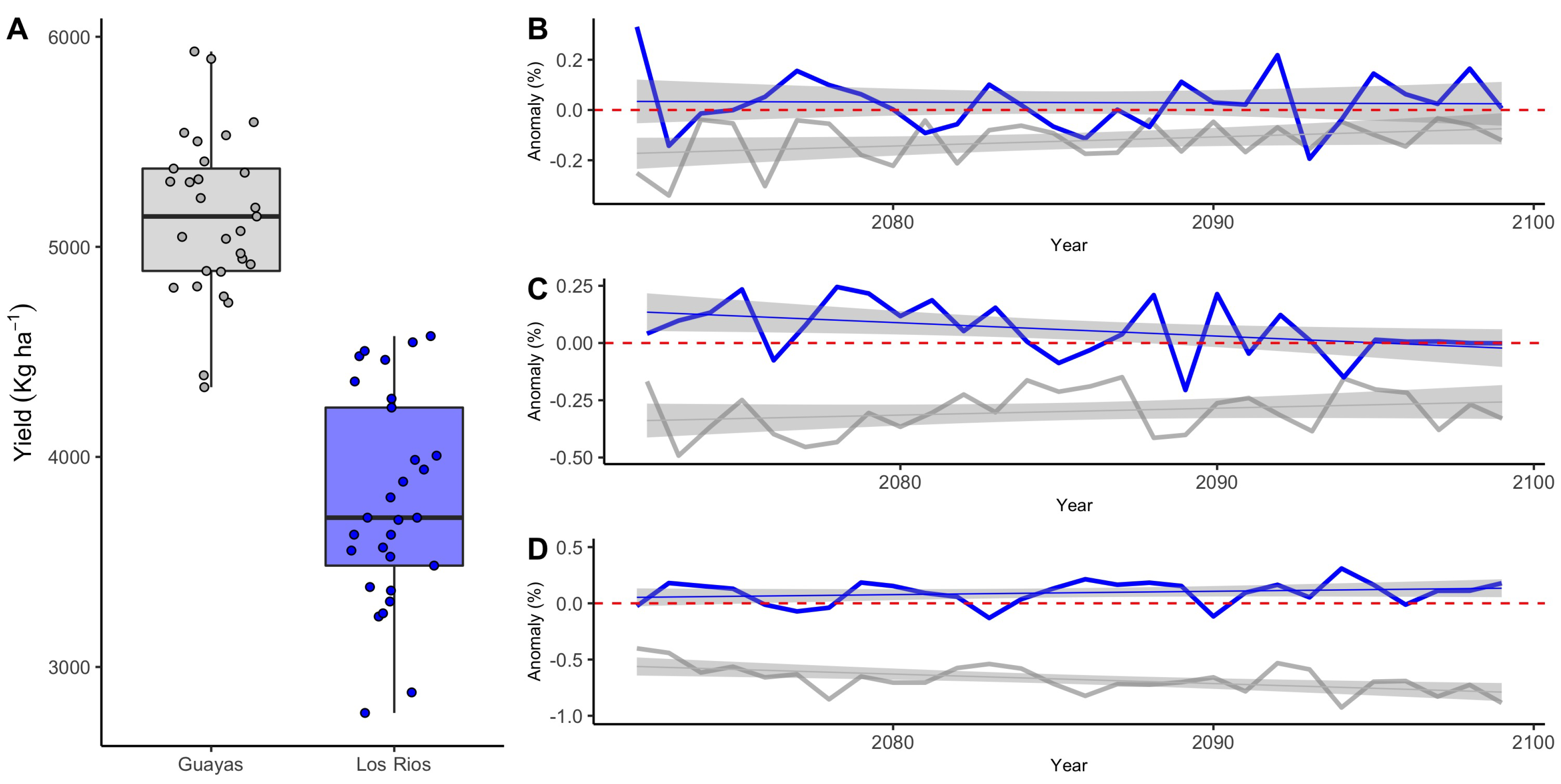
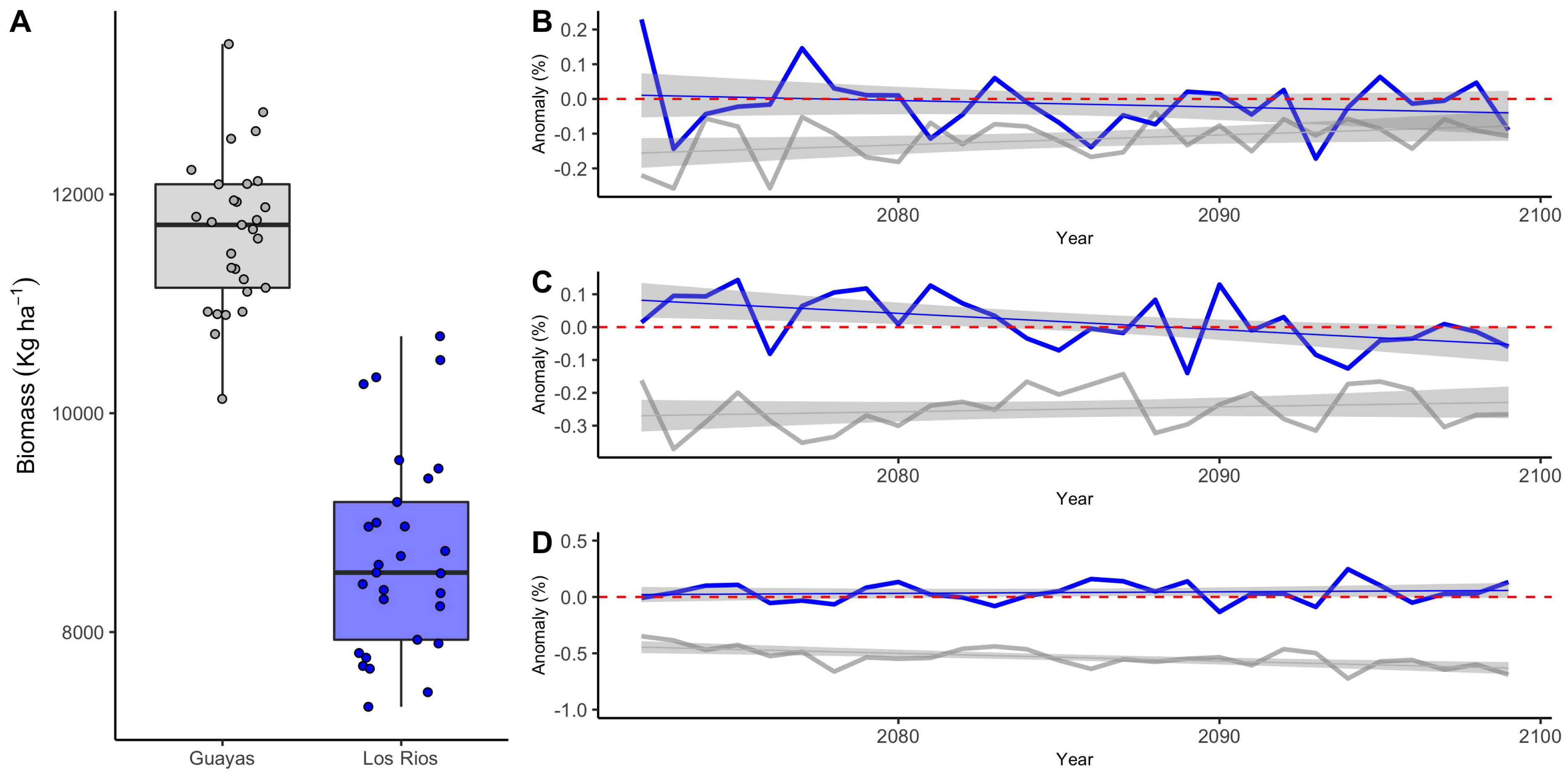
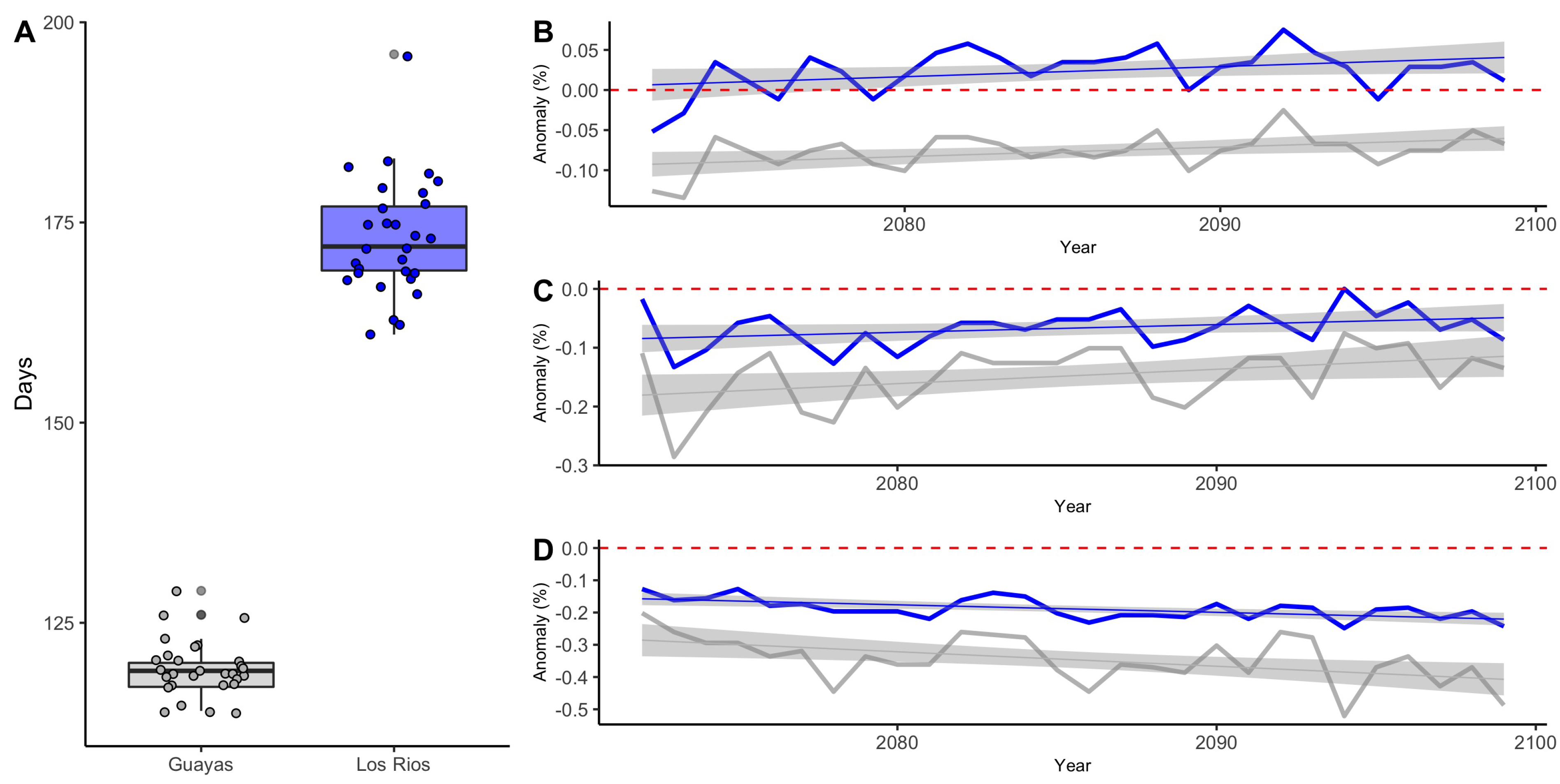
| Yield | Harvest Day | Biomass | |
|---|---|---|---|
| Guayas * | −0.3658 | −0.1902 | −0.3014 |
| RCP 2.6 | −0.1236 | −0.0765 | −0.1168 |
| RCP 4.5 | −0.2982 | −0.1477 | −0.2494 |
| RCP 8.5 | −0.6756 | −0.3463 | −0.5380 |
| Los Rios * | +0.0598 | −0.0773 | +0.0131 |
| RCP 2.6 | +0.0294 | +0.0235 | −0.0148 |
| RCP 4.5 | +0.0563 | −0.0667 | +0.0146 |
| RCP 8.5 | +0.0935 | −0.1889 | +0.0395 |
Publisher’s Note: MDPI stays neutral with regard to jurisdictional claims in published maps and institutional affiliations. |
© 2022 by the authors. Licensee MDPI, Basel, Switzerland. This article is an open access article distributed under the terms and conditions of the Creative Commons Attribution (CC BY) license (https://creativecommons.org/licenses/by/4.0/).
Share and Cite
Portalanza, D.; Horgan, F.G.; Pohlmann, V.; Vianna Cuadra, S.; Torres-Ulloa, M.; Alava, E.; Ferraz, S.; Durigon, A. Potential Impact of Future Climates on Rice Production in Ecuador Determined Using Kobayashi’s ‘Very Simple Model’. Agriculture 2022, 12, 1828. https://doi.org/10.3390/agriculture12111828
Portalanza D, Horgan FG, Pohlmann V, Vianna Cuadra S, Torres-Ulloa M, Alava E, Ferraz S, Durigon A. Potential Impact of Future Climates on Rice Production in Ecuador Determined Using Kobayashi’s ‘Very Simple Model’. Agriculture. 2022; 12(11):1828. https://doi.org/10.3390/agriculture12111828
Chicago/Turabian StylePortalanza, Diego, Finbarr G. Horgan, Valeria Pohlmann, Santiago Vianna Cuadra, Malena Torres-Ulloa, Eduardo Alava, Simone Ferraz, and Angelica Durigon. 2022. "Potential Impact of Future Climates on Rice Production in Ecuador Determined Using Kobayashi’s ‘Very Simple Model’" Agriculture 12, no. 11: 1828. https://doi.org/10.3390/agriculture12111828