1. Introduction
1.1. Background
Rice is a critical food crop worldwide, with lower cultivated area and total production than wheat. In China, rice is grown on approximately 30.08 million hectares, and its production is nearly 211.86 million tonnes [
1]. All aspects of rice cultivation (e.g., planting, field management and harvesting) have been mechanized. In the management of the field, water and fertilizer management, pest and disease control and weed control have created a positive growing environment for rice that takes on a great significance in raising rice production [
2]. At present, the field management model is primarily divided into two types of modes (including manual management and farm machinery management). The manual management mode is subjected to the problems of large time cost and inefficiency. Accordingly, an increasing number of areas are gradually replacing the manual management mode with a farm machinery management mode, such that the demand for mechanization of rice field management is increasingly urgent. Moreover, its sustainable development takes on a critical significance to the green quality of rice production and cost saving and efficiency) [
3].
The image sensor is capable of identifying rice seedlings in the working area ahead of the farm machinery, which obtains the location information of the rice seedlings and builds an accurate operating route for the farm machinery to navigate autonomously between the crop rows [
4]. As a result, accurate extraction of the center line of the crop rows in rice fields serves as a vital technology in the mechanization of rice field management, and a prerequisite for improving the intelligence and automation of agricultural operations.
Rice seedling recognition is dependent on the color features and growth characteristics of seedlings in the image, whereas image quality is often affected by multiple factors, as follows: (1) the different growth postures of rice in the rice field, with branch and leaf cover, which means that different crop rows cover each other in the image; (2) the lack of seedlings in the sowing process which makes the spatial distribution characteristics of crop rows incompletely represented; (3) weeds with similar color characteristics to rice seedlings and growth characteristics, which makes it more difficult to segment weeds and rice seedlings [
5]; (4) unstable lighting conditions in the field, shadows of seedlings under different weather conditions, and excessive light differences which generate more image noises.
1.2. Literature Review
There have been two major approaches to crop row identification. The first approach is based on machine vision and image processing. The color features and growth characteristics of the crop are adopted to segment the crop from the background image and extract information regarding the location of the crop. Tijmen Bakker et al. [
6] proposed an intelligent fusion method based on the grayscale Hough transform to recognize crop rows for beet fields exhibiting high weed density. The collected images were transformed through inverse projection, the images were grayed, and the crop information was extracted from the segmented a priori image information, respectively. Lastly, the crop row straight lines were extracted through Hough transform. The experiments have confirmed that the method has a crop row localization error of 22 mm, though the method is subjected to the problem of recognition error increasing when the camera is overexposed and the weed density is too high; Ng Tong [
7] applied the Artificial bee colony algorithm to rice row recognition. The image was preprocessed with optimized 2G-R-B and Otsu to obtain a feature map of rice seedlings, and the feature map was clustered using the Artificial bee colony algorithm and least-squares method to extract rice rows in a straight line. The experimental result has indicated that the recognition accuracy of this method is 91%, with an average time consumption of 78.2 ms, which can meet the actual agricultural machinery use requirements. Jiqing Chen et al. [
8] solved the problem of high computational effort and low accuracy of conventional algorithms using the Hough transform-based navigation line extraction method for prediction points. Zenghong Ma et al. [
9] proposed a crop root row detection method for rice fields using linear clustering and supervised schools. First, the crop information is extracted by a combination of vegetation index method and dynamic threshold segmentation, followed by the use of the horizontal banding method to obtain the number of crop rows in the image. Linear clustering algorithms and outlier detection mechanisms are employed to obtain the actual crop rows in the image and remove invalid rows on both sides of the image. Lastly, a parametric regression equation for the distance between crop rows and crop roots is solved through supervised learning to obtain the crop root rows. In brief, both machine vision and image processing-based methods are dependent on the color characteristics of the crop, thus becoming highly sensitive to the color characteristics of the crop. When the green features of the crop are more intense, the segmentation of the background and the crop achieves good results. Besides, when the environmental light source changes or the weed density is denser, the method’s results tend to have more significant errors.
With the continued development of Deep Learning in a wide variety of fields over the past few years, the AlexNet Network proposed by Krizhevsky et al. [
10] in the ImageNet [
11] image classification competition has outperformed the conventional machine vision-based methods in terms of accuracy in image classification. In the computer vision field, Deep Learning has developed three mainstream directions in terms of the Convolutional Neural Network, including (1) the target detection models (e.g., SSD [
12], Fast R-CNN [
13], and YOLO [
14,
15,
16]); (2) the semi-semantic segmentation models (e.g., U-Net [
17] and DeepLab [
18]); (3) the instance segmentation models (e.g., Mask R-CNN [
19] and YOLACT [
20]). A growing number of scholars are applying Deep Learning to crop row recognition because of Deep Learning’s robustness and strong feature extraction. Wang [
21] proposed a YOLOv3 [
18]-based method for rice row seedling column detection. The seedling detection frame output from the model was adaptively clustered, followed by the extraction of center line feature points using the SUSAN algorithm with detection frames based on the same row of seedlings, as well as the fitting of seedling center lines using the least-squares method. The experimental results confirm that the algorithm takes an average of 82.6ms to meet the real-time requirements of agricultural navigation in a simulated paddy field environment; Shyam P. Adhikari et al. [
22,
23] presented a method to detect crop rows in rice fields based on semantic graphics. The ESNet model with an encoder-decoder structure was trained using simple semantic images for end-to-end extraction of crop rows in a paddy field. The results have suggested that the method is efficient in extracting crop row information accurately, thus guiding the weeder to navigate autonomously along the crop rows in the paddy field; Wang Shanshan et al. [
24,
25] proposed a method to identify rice seedling rows in accordance with the Neighborhood Hough Transform of feature points. The feature points of rice seedlings were detected through Fast R-CNN network, and the center line of the seedling rows was identified using the Neighborhood Hough Transformation algorithm. The method effectively solves the effect on crop row detection due to weed density, light intensity variation and seedling row curvature variation in the paddy field, and then the team proposes the method of rice seedling row detection through row vector grid-based classification. The problem of image recognition of seedling location information is transformed into a row vector network classification problem with global features. The method effectively reduces the effect of degradation of captured image quality due to floating weeds in the paddy field and farm machinery jittering, and it exhibits the features of low computational effort and high accuracy compared with other types of networks. Accordingly, the above research shows that the crop row recognition method using the Convolutional Neural Network can overcome the problems of weak ability to extract color features and poor adaptability to the environment in conventional image processing.
1.3. Contributions
Outdoor crop row detection in rice fields is affected by a wide variety of factors (e.g., weed density in the rice growing environment, unstable lighting conditions in the farmland, water reflections and lack of seedlings in the crop rows). Although the conventional methods of machine vision and image processing to recognize rice seedling rows from color features and threshold segmentation are capable of extracting the information of crop rows in farmland relatively accurately, there are the problems of poor robustness and low accuracy rates in complex farmland environments, which cannot meet the requirements of practical agricultural machinery in field operation. However, the Convolutional Neural Network has the ability to overcome the shortcomings of the conventional image processing methods by achieving outstanding extraction of features in both normal and complex environments. Generally, the object detection model is used to accurately identify and locate rice seedlings. The characteristic points of the seedlings are grouped into a particular crop row by means of a classification or clustering algorithm. Eventually, the center line of each row is detected in accordance with the feature points of the respective cluster after clustering.
However, the above methods have the problem of single-feature information by relying only on the Convolutional Neural Network or machine vision depending on the crop growth characteristics and color features extracted, such that a method is proposed for rice seedling row recognition based on a Gaussian Heatmap. The CNN Model consists of the Feature Extraction Module, the Heatmap Regression Module, and the Grid Offset Module. The method takes the rice seedling image as the CNN model input and the key points on the center line of the crop rows as the output. Through transforming the rows of rice seedlings in the image into a scatter plot with continuity distribution features, the CNN Model is led to learn the color features and continuity distribution features of rice seedlings during training.
The rest of the paper is as follows: the proposed methodology is explained in
Section 2, and the experiments and results analysis of the CNN model on the relevant dataset are described in
Section 3. The conclusion is included in
Section 4.
2. Materials and Methods
In the present section, rice seedling row identification based on a Gaussian Heatmap is introduced. To be specific, image acquisition and annotation, the structure of the Network Model and the definition of the loss function are elucidated.
2.1. Image Acquisition
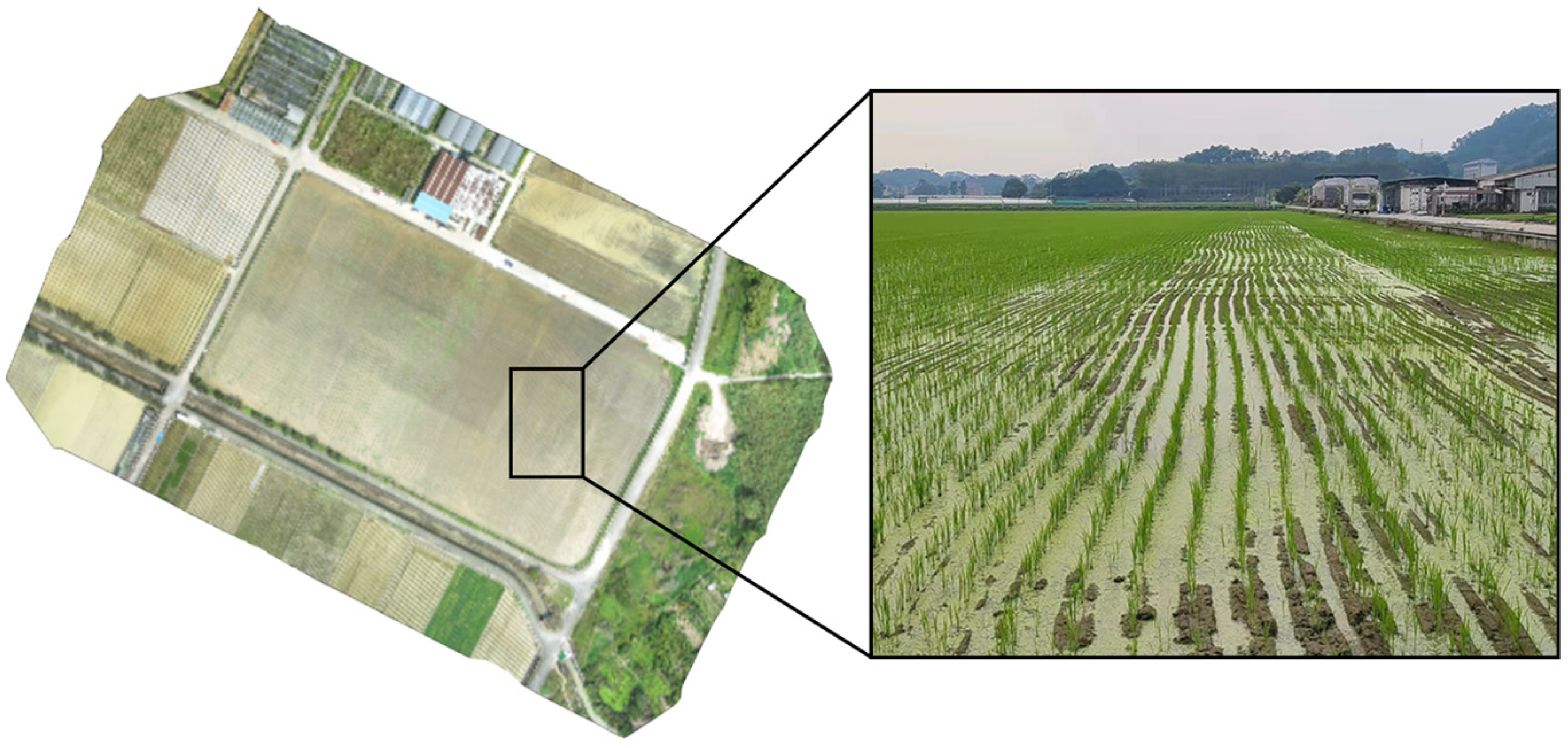
Generally, weeds growth between the 25th and 30th day following the transplanting of the rice seedlings. Thus, the camera was installed at a distance of approximately 1.2 m from the ground to simulate the image scenario during the actual farming operation, and the angle between the camera and the horizontal plane was 35–60 degrees to capture the images of the rice seedlings. The images were taken on the 30th day after transplanting, when the height of the rice seedlings was nearly 18–22 cm, and the row spacing of the rice seedlings was 25 cm. A total of 2608 images were captured using the Eimage Seiki DFK 21BU04 color camera(The Imaging Source, Taipei, Taiwan Province, China) at an image resolution of 640 * 480 under cloudy and sunny skies in an unmanned farm rice field (as shown on
Figure 1) at the Teaching and Research Base of South China Agricultural University in Zengcheng District, Guangzhou City, Guangdong Province, China, in April 2022.
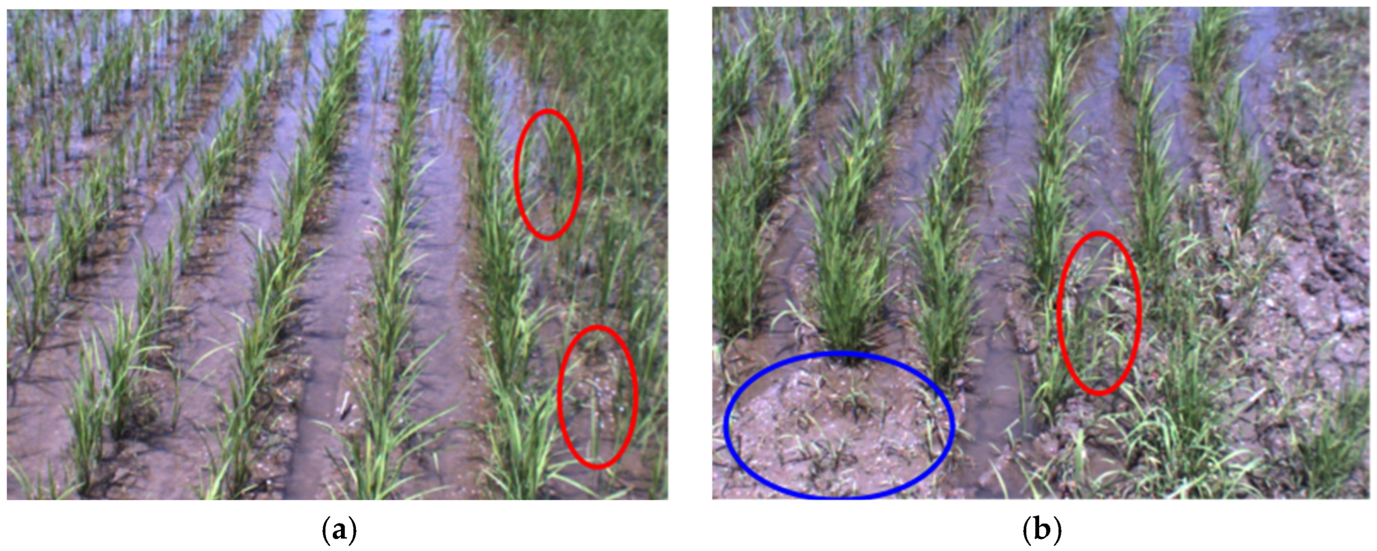
Figure 2 presents the different images taken of rice seedlings.
Figure 2a presents an image of a rice seedling under clear skies. As depicted in the figure, the seedlings and the weeds at the boundary of the rice field overlapped each other.
Figure 2b presents an image of a rice seedling under a cloudy sky. As depicted in the figure, the weeds and seedlings had similar color characteristics, the weeds and seedlings were overlapping each other in the image, and there were missing seedlings in the crop row. The red circles in
Figure 2 represent the location of weeds, and the blue circles represent the location of lacking seedlings.
2.2. Generation Dataset
The proposed CNN Model takes the key points on the center line of the crop rows as the output. Therefore, according to the distribution pattern of the rice seedling rows in the image, the generated dataset was labelled with the following rules: (1) the position of the crop row’s center points were set to the roots of the rice seedlings; (2) the center line of the crop rows were labelled using the method of broken lines; (3) equal distance horizontal splines were used for the broken lines to cut to generate the scatter plot with continuous distribution characteristics; (4) the corresponding Heatmap was generated from the scatter plot and the 2D Gaussian function (Formula (1)) and the generated Heatmap was presented as the dataset for the rice seedling rows.
Figure 3a illustrates the use of the broken lines to label the rice seedling rows,
Figure 3b presents the annotated key point image, and
Figure 3c represents the generated Heatmap. The Gaussian function is described as follows:
where
in Formula (1) represents the radius of the Gaussian kernel,
and
represent the central coordinate points of the template match.
2.3. Network Architecture
In this study, a method is proposed to identify rows of rice seedlings based on a Gaussian Heatmap by inputting images of seedlings in a paddy field and outputting all key points on the respective row from a network model. There are currently two mainstream methods for learning the absolute coordinates of the respective key point on the image using the Convolutional Neural Network [
26]. The first method refers to a direct regression of the absolute coordinates of the respective key point based on full connectivity, which enables end-to-end full differential training but lacks spatial generalization capability. When the key points in the dataset are concentrated at a certain location in the image, only the information of local features in the image will be activated in the fully connected layer. On that basis, the Neural Network will not be trained accurately and adequately on the global features, besides possibly making the network overfit. The second method is based on the 2D Gaussian Heatmap to obtain the exact coordinates of the key points, which are generated by the convolutional layer, while the absolute position of the key points refers to the position where the Heatmap is significantly activated. Compared with the first method, the second method is dependent on the strong feature extraction property of the convolutional neural network, allowing the convolutional neural network to learn the global feature correlation between key points, and in addition using a Gaussian function to generate a “soft annotation” based on the 2D Gaussian Heatmap annotation. Thus, the convolutional neural networks are enabled to learn more accurately and adequately. However, as depicted in the schematic diagram of the Gaussian Heatmap error in
Figure 4, typical 2D Gaussian Heatmap resolution accounts for 1/4 of the original input image resolution. When the coordinates of the selected key points are mapped to the original image size through upsampling after filtering, there is an error between the remapped coordinates and the Ground Truth coordinates.
Accordingly, a method is proposed in this study for a Gaussian Heatmap-based key point regression module based on a Gaussian Heatmap and the Grid Offset Module in accordance with the YOLO series of the Object Detection Network. YOLO adopts an Anchor-based frame and Grid Offset Module to accurately localize the centroid position of target points in an image. The method requires predicting the offset of the respective grid point in the
x-axis and
y-axis directions, thus keeping the reference value of the predicted offset within a small range, which is beneficial for increasing the network learning accuracy. On that basis, a Gaussian Heatmap is combined with the Grid Offset Module.
Figure 5 depicts a schematic diagram of the Gaussian Heatmap and the Grid Offset Module. The Gaussian Heatmap outputs the coordinate position of the respective key point, and the Grid Offset Module finds the offset in the
x-axis and
y-axis directions of the corresponding grid position to be in accordance with the coordinate position of the key point and obtains the exact coordinate position of the key point after upsampling.
In order to improve the accuracy of the model prediction results while preventing the problem of disappearance or explosion of the gradient as the model reaches deeper layers, we use HRNet_w18 [
27] as the backbone feature extraction network of the model in this study. As showed in
Figure 6 of Network Model, the HRNet_w18 backbone feature extraction network comprises the Stem Net Module, the Basic Conv Module, as well as the High-Resolution Convolution Module. To be specific, (1) the Stem Net Module and Basic Conv Module perform high-resolution feature extraction on the input image. (2) The High-Resolution Convolution Module strengthens and extracts the feature layers; its core function is to use convolution and stacking at multiple resolutions to keep the input features significantly activated at different resolutions during the forward inference of the network, and the perceptual field is capable of effectively enhancing the network’s ability to extract features in the global space, so that the feature layers can also have the characteristics of guaranteed high-resolution and strong activation of features when the network is deep. As shown in Stage 2, Stage 3 and Stage 4 in
Figure 6, the High-Resolution Convolution module takes the output of the previous convolution as input and performs Basic Block 4 times on the input feature layers, respectively (as shown in
Figure 7). Basic Block mainly includes 2 convolution layers and 1 skip module; the feature layers are fused with the original feature layers after 2 convolutions to enhance the information of the extracted features while avoiding disappearance and explosion of the gradient. Moreover, in the final stage of the High-Resolution Convolution Module, the feature layers with low resolution are fused with the feature layers with high-resolution by upsampling, while the feature layers with high-resolution are fused with the feature layers with low resolution by downsampling. The model is extended in width while being deepened, making the model more accurate for the extraction of features. (3) The Multi-Scale Fusion Module accounts for fusing the feature layers that have gone through the high-resolution convolution module from low-to-high stacking and outputting the feature layers with high resolution. (4) The Output Module creates Heatmap branches and Grid Offsets Model from the High-Resolution Convolution Module, followed by use of the above-proposed regression key point absolute position method to extract the key point positions of the respective row in the image.
Table 1 presents the sizes of the input and output layers for each feature layer from the proposed model.
2.4. Loss Functions
The Network Loss Function used in this study consists of two main components, including: Heatmap Loss and Grid Offset Loss.
For Heatmap Loss, the network should result in a series of consecutive point sets after forward inference of the network since the network ends up with a result of consecutive key points on the respective crop row on the image. However, the above contiguous points account for a relatively small number of pixels on the whole image, leaving an imbalance in the number of positive and negative samples of key points at the pixel level of the image. When the number of negative samples is significantly larger than that of positive samples, the direction of network optimization is shifted, and it becomes more difficult to train the network. Thus, an improved Focal Loss [
28] is employed as the loss function for the heat map based on the method of calculating loss for Gaussian Heatmap in CenterNet [
29]. The loss function formula is expressed as follows:
where
N denotes the number of key points in the image;
represents all coordinate points on the Heatmap;
is the predicted result of the network model;
denotes the Ground Truth;
and
represent the hyperparameters of Focal Loss, which are 2 and 4, respectively.
Since the labelling format is a point-labelling format based on Gaussian functions, there are two different cases for the Focal Loss calculation.
(1) For the coordinate point at , i.e., the point at the center of the Gaussian kernel. When is close to 1, i.e., the point is an easily divisible sample and the calculated value of the scale factor is a smaller value, thus fine-tuning the network as a whole. In contrast, when tends to 0, i.e., the point is a difficult sample, the calculated value of the scale factor is a larger value, thus increasing the training weight of the network for this one point.
(2) Likewise, for coordinate points of , i.e., points that are not the center of the Gaussian kernel, the loss values of positive and negative samples are penalized using a scale factor , while the loss weight of negative samples around the center of the kernel is reduced by a distance factor .
For the Grid Offset Loss, since the feature layer undergoes 4-fold downsampling during network forward inference which results in discretization errors in the coordinate positions of key points, the L1 regularized loss function is adopted to calculate the loss values for the offsets of the predicted centroids as follows:
where
N denotes the number of key points in the image;
is the predicted result of the network model;
is the Ground Truth.
is only for the calculation of the key point position offset error loss; other offset losses that are not key point positions are not calculated. The loss function formula is expressed as follows:
3. Experiments and Results
In this section, we mainly describe the experiments performed on the proposed method on the rice seedling row dataset, with the main contents including: (1) experimental setup; (2) ablation experiments; (3) analysis of experimental results.
3.1. Experimental Setup
3.1.1. Description of the Dataset
To evaluate the model approach proposed in this study, a rice row dataset was set, including 2608 images of rice rows in different weed environments. 90% of the dataset images served as the training set and validation set for the network, with the ratio of the training set to the validation set at 9:1. The remaining 10% of the dataset images served as the test set. In addition, the rice row dataset comprised three scenarios (including normal scenario, missing seedlings scenario and weed scenario), with a uniform resolution of 640 * 480, and the number of rice rows to be identified in the respective image was 4 to 6.
3.1.2. Hardware and Software Setup
The hardware configuration employed for training all models in this study included the AMD Ryzen5 3600 processor at 3.6Ghz (Advanced Micro Devices, Inc., Santa Clara, CA, USA), GDDR4 memory with 16GB of RAM and the NVIDIA GeForce GTX 1650 graphics card with 4GB of video memory (NVIDIA, Santa Clara, CA, USA). The Deep Learning environment was built using CUDA 10.1, CUDNN 7.6.5, Python 3.8, as well as TensorFlow-GPU 2.3.0 (Google, Mountain View, CA, USA). The training parameters of the model were as follows: the initial learning rate of the network reached 0.001; the learning rate decreased in this mode as stratification decreased learning rate; the decay weight factor of 0.0001; the optimizer was the Adam algorithm; with a momentum factor of 0.9, the initial number of iterations was set to 100 epochs; the Gaussian kernel radius size was set to 5; and the training set was to stop early when the loss value of the training set did not decrease.
3.1.3. Model Evaluation Criteria
The following three metrics were employed as evaluation criteria for all models in this study. This includes
PCK (Percentage of Correct Key points) [
30],
APO (Average Pixel Offset), and Network Inference Speed.
PCK is defined as follows:
where
in formula 5 represents the number of actual true values,
denotes whether the key point matches the true value,
expresses the location of the model prediction key,
is the Ground Truth that the Predict Result matches, and
is the matching threshold. In this study, since the number of points predicted by the network model will generally be greater than the number of true values, the Hungarian matching algorithm [
31] was used to match the Ground Truth and the Predict Result. The model predicted all the predicted points and all the points of the true value through the Eulerian distance to build the corresponding cost matrix, and thus that the respective true value matched only one predicted value. The coordinates of a point in the image predicted by the model were set to
, and the coordinates of the true value it matches were set to
. If the Eulerian distance between the two is less than a set threshold
, the prediction is considered correct; otherwise, the prediction is incorrect.
PCK represents the number of correct results predicted by the model as a proportion of the number of true values.
APO is defined as follows:
where
N denotes the number of key points after a successful match;
represent the Ground Truth;
are the coordinates of the Predict Result matching the Ground Truth after passing the Hungarian matching algorithm. This metric reflects the average offset of the model at the pixel level of the predicted points. If the average offset is smaller, the more accurate the model prediction will be considered; otherwise, the less accurate the model prediction will be considered.
Network Inference Speed is the time taken to count the time for the input image to the network model, the network model to compute the inference, as well as the network to output the result. If the time is shorter, the model is considered have a higher efficiency and higher real-time performance in forward inference.
3.2. Ablation Experiment
In the present section, the following main ablation experiments were performed: (1) comparison of different horizontal spline settings on model prediction performance; (2) comparison of different backbone network models on model prediction performance; (3) comparison with state-of-the-art object detection models.
3.2.1. Comparison of Model Prediction Performance with Different Number of Horizontal Splines
The method uses horizontal spline cuts for the folded segments in the annotated image to obtain a series of key point maps. Accordingly, the different location and spacing distribution relationships of individual key points also had different effects on the method proposed in this study. The effect of cutting the fold segments with different numbers of horizontal splines on the performance of the algorithm model was explored. Since the resolution of the images used was 640 * 480, the number of horizontal strips was set to 20, 30, 40, 50 and 60, i.e., 24, 16, 12, 9 and 8 pixels between the key points, to train the network model. The network model was trained with the same parameters as in
Section 3.1.2 above, and the results are listed in the
Table 2.
From the results in
Table 2, the algorithm’s prediction results were poor when the number of horizontal strips was 50 and 60, i.e., the interval between key points was 8 and 9 pixels, respectively, and the
PCK of the network model was 66.22% and 49.217, respectively, with an Average Pixel Offset of 3.572 and 3.175 pixels. When the number of horizontal strips was 40, i.e., the interval between key points was 12, the
PCK and
APO were 93.726% and 3.08 pixels, respectively, when the number of horizontal strips was set to 20 and 30, i.e., 24 and 16 pixels between key points, with 91.392%, 3.277 pixels. Compared with the group set to 40 horizontal strips, the
PCK decreased by 0.432% and 2.334% respectively, and
APO differed by 0.115 and 0.197 pixels respectively. Thus, when the number of horizontal strips is set too high, the key points will be lost in the upsampling, thus reducing the prediction performance of the network and the completion rate of the network. The network prediction results are not spatially continuous. Accordingly, in this study, we choose to set 40 horizontal strips to cut the folded segments of the image in
Figure 1 to obtain the optimal prediction results.
3.2.2. Comparison of Model Prediction Performance of Different Backbone Networks
In the second ablation experiment, the prediction performance of different backbone feature extraction networks was compared to network models, where the performance metrics included
PCK,
APO, Number of Network Parameters, as well as Network Inference Speed. The backbone feature extraction networks applied included HRNet_w18, HRNet_w32, HRNet_w48, ResNet50 [
32], VGG16 [
33] and CSPDarkNet53 [
34].
Table 3 lists the comparison results. As depicted in
Table 2, HRNet networks outperformed ResNet50, VGG16 and CspDarkNet53 in
PCK,
APO and Network Inference Speed. Furthermore, HRNet with different channel counts improved the
PCK by 50.814% to 54.004% over ResNet50, VGG16, and CspDarkNet53 networks, respectively, and improved the
APO by 0.939 to 1.45 pixels.
Moreover, the prediction performance of HRNet structures with different number of channels was compared. The results indicated that the number of HRNet_w18 parameters decreased by 66.5%~84.7% compared with HRNet_w32 and HRNet_w48, respectively, and the HRNet_w18 structure achieved the optimal prediction performance in the rice row test set. When the pixel threshold was at 10 pixels, the HRNet_w18’s PCK and APO were 93.726% and 3.08 pixels, respectively. Furthermore, the average prediction time of HRNet_w18 was 45.4 ms, i.e., 22FPS. Although HRNet_w32 and HRNet_w48 had more complex and deeper High-resolution Convolution Module, their prediction performance was lower than that of the HRNet_w18 structure. The PCK and APO of HRNet_w32 and HRNet_w48 were 91.498%, 92.072% and 3.279 pixels, 3.291 pixels respectively, which are 2.228%, 1.654% and 0.199 pixels, 0.211 pixels different from HRNet_w18, and the average prediction times are 63.8ms and 102ms respectively, which are 1.4 times and 2.24 times of HRNet_w18. Therefore, we choose HRNet_w18 as the backbone feature extraction network for the model in this paper.
3.2.3. Comparison with State-of-the-Art Object Detection Models
Due to the better recognition and localization effect of object detection models, most crop row recognition methods based on Deep Learning have used object detection models in recent years. State-of-the-art object detection mainly includes: (1) One-stage models, mainly including YOLOV4, SSD [
12], etc.; (2) Two-stage models, which include Faster RCNN [
13], etc.; (3) Anchor-free models, for instance, FCOS [
35], etc. The CNN Models proposed in this paper was compared with the state-of-the-art models mentioned above. The comparison results are shown in
Table 4. From
Table 4, it can been obtained that the proposed method performs better than the above state-of-the-art object detection models for both
PCK and
APO metrics in the test set. Moreover, except for SSD, the CNN model proposed achieves 1 to 3 times faster Network Inference Speed than the other models.
3.3. Analysis of Experimental Results
3.3.1. Visualizing Network Results
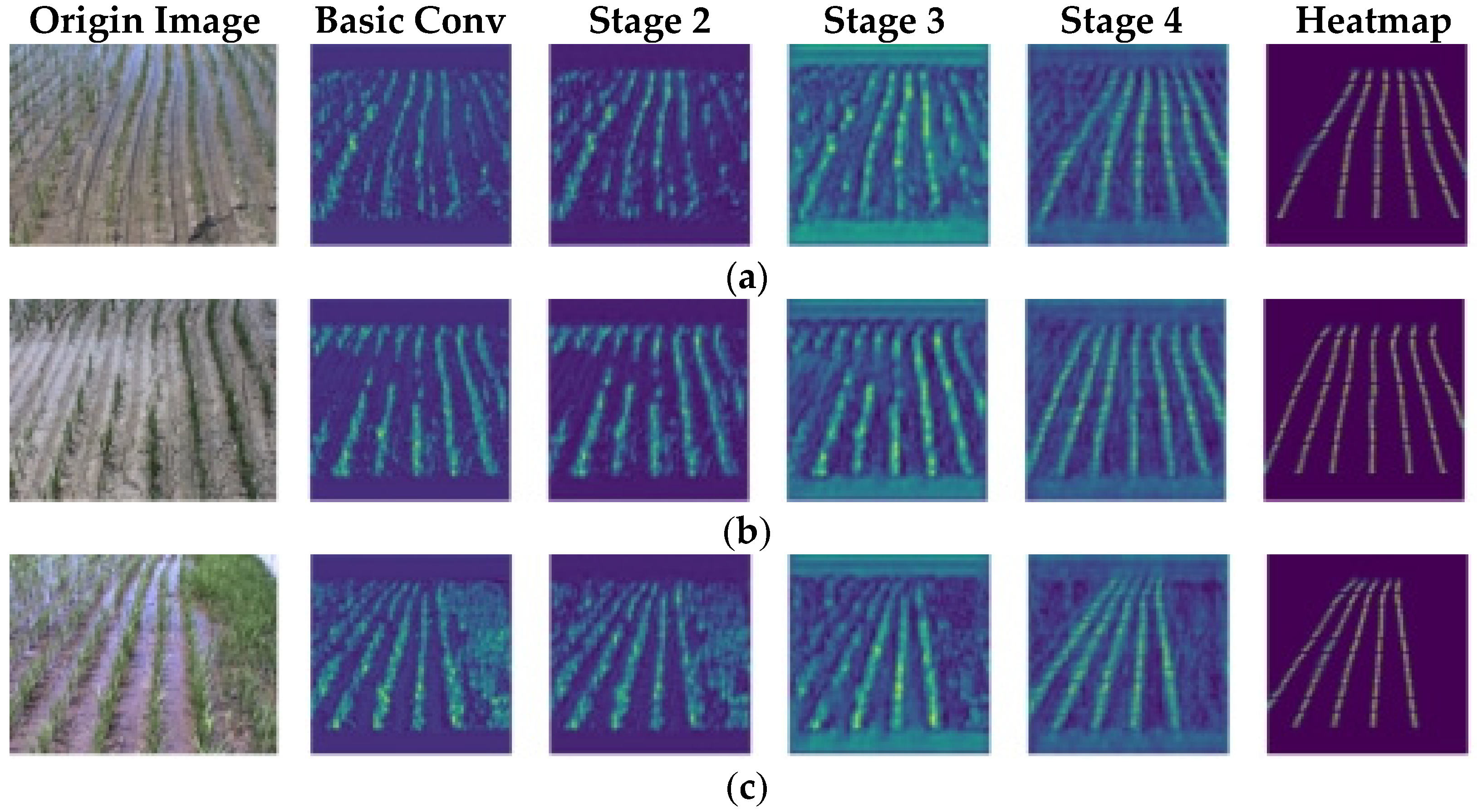
The Gaussian Heatmap based rice row recognition method proposed in this study is an end-to-end network, i.e., the input image is input, and the network automatically recognizes the information from the key points of the respective row. The visualization network is used in this study as a non-parametric method to account for the extraction of different features in the middle layer of the model during forward inference [
36].
In this study, the rice row images in the three scenarios mentioned above are used as model input, and the high-resolution feature layer and Heatmap feature layer in the output layers of Basic Conv, Stage 2, Stage 3 and Stage 4 in
Table 1 above are visualized and analyzed respectively, and the feature visualization results of the intermediate layer are obtained by calculating the convolution layers of the different channels and accumulating them.
Figure 8 shows that the first image on the left is the original image of the input model, and the second to sixth images correspond to the visualization results of Basic Conv, Stage 2, Stage 3, Stage 4 and Heatmap layers. The visualization results show that Basci Conv and Stage 2 in the shallow network learn the green features and edge features of the rice rows in the image; Stage 3 learns more complex features such as the distinction between rice rows and weeds, as well as the distinction between rice rows and the background; Stage 4 in the deeper network extracts the continuous relationships and position relationships of key points in the respective rice row. The final output of the Heatmap layer shows the results of the model learning compared to the original ma. As shown in
Figure 8, the green pixels represent the locations of the key points in the rice rows in the original map, which are the areas with strong negative activation in the Heatmap layer, while the blue pixels represent the locations of the background in the original map, which are the areas with strong negative activation.
The visualization results show that the proposed method can enable the network to effectively learn the color features and spatial distribution features of the rice rows. Compared with conventional image processing algorithms, the Gaussian Heatmap-based rice row recognition method can effectively reduce the effect of weeds or missing seedlings in rice rows on the effectiveness of rice row recognition.
3.3.2. Performance of Network Models in Different Rice Environments
In the Test Set, there were 261 images, of which 104 were in the Normal scene, 97 were with weeds in the rice rows, and 64 were with lack of seedlings in the rice rows. In this study, the network prediction results of the Test Set of rice row images for each of the above three scenarios were compared. The comparison results are listed in
Table 5.
As depicted in
Table 5, among the three tested sceneries, the sceneries with lack of seedlings had the lowest
PCK of the network prediction results, with a
PCK of 91.48%. The other two scenarios, the Normal scene and the Weed scene, had closer
PCKs of 94.33% and 94.36%, respectively. Additionally,
APO was relatively similar for all three scenes tested, at 3.09, 3.05 and 3.13 pixels, respectively.
Figure 9 shows the test results for the three scenes, where
Figure 9a–c show the test results for the Normal scene, Weed scene and Lack of seedlings scene respectively. The black points in the figure are the results of the key points predicted by the model. As depicted in
Figure 9, the key points predicted by the model in the three scenarios had uniform and continuous distribution on the image, and the respective key point was distributed on the rice rows. This suggests that the model proposed in this study has effectively learned the color characteristics and spatial distribution characteristics of the rice rows. As depicted in
Figure 9b, the red circle shows that in the longer rice rows, the proposed method is capable of effectively separating the rice rows though it is already difficult to distinguish different rice rows visually at the far end. In the weed scene, as depicted in
Figure 9b yellow circles, although the weeds and rice rows at the edges of the image had similar color characteristics and were masked to varying degrees from the rice rows in the image, the model also produced more accurate rice row recognition results based on the spatial distributivity of the rice rows. In the case of a missing seedling scenario, as shown in the green circle in
Figure 9c, the methodology also obtains relatively accurate results when crop row continuity features are incomplete due to the lack of seedlings. The network model also performed well in curved rice rows as shown in the blue circle in
Figure 9c.
3.3.3. Analysis of the Reasons for Mistaken Prediction Results
We have analyzed cases where the model prediction accuracy was low in a seedling-deficient environment and a weedy environment.
Figure 10a,b present the two cases where low prediction accuracy occurred. The black pixels in the figure represent the model prediction results, and the green pixels represent the real key points marked. In the missing rice environment, shown in the yellow circle in
Figure 10a, when the distribution of rice in the rows was sparse and the color characteristics of the rice were blurred, there was a small pixel deviation between the Ground Truth and the model-predicted key points, with an average pixel offset of no more than 15 pixels. In the weedy environment, as presented in the red circle in
Figure 10b, when there was a small area of weeds at the edge of the image that obscures the position of the rice rows, there was a large pixel deviation between the Ground Truth and the model-predicted key points, with an average pixel offset of no more than 25 pixels. At this point, there was a large deviation between the crop rows predicted by the model and the actual crop rows.
4. Conclusions
In this study, we propose a new method for identification of rice seedling rows. First, we have analyzed the research on recognition of rice seedling rows in recent years, and summarized the strengths and weaknesses of different methods, including the conventional machine vision and the Convolutional Neural Network, in the recognition of crop rows. It was found that the above-mentioned research have the problem of single information of features for the extraction of rice seedling rows, therefore, a method of rice seedling row recognition based on a Gaussian Heatmap is proposed. Secondly, the rice seedling row dataset was built by field photography in different environments such as Normal scene, Lack of seedling scene and Weed scene. The annotation of rice row key points is obtained by cutting the respective rice row with a horizontal spline. To further strengthen the extraction of features while avoiding the problem of disappearance and explosion of gradients, the CNN model based on a feature extraction network with the High-Resolution Convolution Module and the Gaussian Heatmap-based key point regression module is built. In addition, the CNN Model uses Focal loss and L1 regularization as the Heatmap loss function and the Grid Offset loss function which can effectively decrease the effect of imbalance between positive and negative samples in the prediction results, thus leading the model to learn the characteristics of color and continuity distribution of rice seedling rows.
The visualization analysis confirms that the model can effectively learn the color characteristics and spatial distribution of rice rows on the image, effectively reducing the effect of recognizing rice rows due to changes in ambient light, weed cover in rice rows or rice rows missing seedlings and others, and the model exhibits better robustness for rice rows in different environments.
The visualization analysis confirms that the CNN Model is capable of combining the extracted information from each of the various feature layers with different resolutions, including the distribution of rice seedling rows and the differentiation between rice rows and the background, in a complex farming environment where there are ambient light changes, weed cover in the rice field, or widespread lack of seedlings in the rice field, resulting in a highly accurate and continuous distribution of rice seedling row features. Therefore, the model is considered to effectively learn the color characteristics and spatial distribution of rice rows on the image, effectively reducing the effect of recognizing rice rows due to changes in ambient light, weed cover in rice rows or rice rows missing seedlings and others, and the model exhibits better robustness for rice rows in different environments.
The results of the proposed model on the rice row dataset suggest that when the model employs HRNet_w18 as the feature extraction network and cuts the rice row fold annotation with 40 horizontal splines, the model is capable of achieving a PCK of 93.726% and APO of 3.08 pixels, and the Network Inference Speed of 22 FPS. Moreover, the proposed model performs significantly better than the current object detection models in terms of evaluation metrics in the test set by comparing with the state-of-the-art object detection model.
In conclusion, the model proposed in this study converts the problem of recognition of rice seedling rows into the recognition of feature points with continuous distribution characteristics in rice seedling rows, and achieves the end-to-end output of the model, while simplifying the flow of the algorithm. The experimental results proved that the model could satisfy the practical agricultural machinery in row operation for the crop rows to be identified in real time and accurately.
In the future, there will be focus on converting the model results to practical navigation center lines for farm machinery and deploying the model on edge computing devices such as the NVIDIA Jetson Tx2, to achieve high-quality navigation for farm machinery in the field.
Author Contributions
Conceptualization, Z.Z. and X.L.; methodology, R.H. and W.Z.; software, R.H.; validation, R.H. and C.J.; formal analysis, C.J.; investigation, R.H. and B.Y.; resources, R.H. and W.Z.; data curation, R.H.; writing—original draft preparation, R.H.; writing—review and editing, W.Z. and Z.Z.; visualization, B.Y.; supervision, X.L.; project administration, Z.Z.; funding acquisition, Z.Z. All authors have read and agreed to the published version of the manuscript.
Funding
This research was funded by the National Natural Science Foundation of China (no. 32071914) and Basic and Applied Research Fund of Guangdong Province of China (no. 2019A1515111152).
Institutional Review Board Statement
Not applicable.
Data Availability Statement
All data are presented in this article in the form of figures and tables.
Acknowledgments
The authors gratefully acknowledge the editors and anonymous reviewers for their constructive comments on our manuscript.
Conflicts of Interest
The authors declare no conflict of interest.
References
- Zhong, Z.P.; Sun, S.; Xu, S.W. Analysis of China’s Grain Supply and Demand in 2020 and Its Future Prospects. Agric. Outlook 2021, 17, 12. [Google Scholar] [CrossRef]
- Shi, S. Research on Rice Planting Technology and Field Management. Guangdong Seric. 2021, 55, 80–81. [Google Scholar]
- Yuan, F.; Ye, X.; Liang, S.; Song, Y.; Nie, H.; Yao, J. Recommended Pattern of Rice Production Mechanizationin Guandong Province. Mod. Agric. Equip. 2021, 42, 79–82. [Google Scholar]
- Li, H.; Li, Z.; Dong, W.; Cao, X.; Wen, Z.; Xiao, R.; Wei, Y.; Zeng, H.; Ma, X. An Automatic Approach for Detecting Seedlings per Hill of Machine-Transplanted Hybrid Rice Utilizing Machine Vision. Comput. Electron. Agric. 2021, 185, 106178. [Google Scholar] [CrossRef]
- De, Q.; Liao, J.; Wang, Y.; Yin, J.; Zhang, S.; Liu, L. Detection of Seedling Row Centerlines Based on Sub-Regional Feature Points Clustering. Trans. Chin. Soc. Agric. Mach. 2019, 50, 8. [Google Scholar] [CrossRef]
- Bakker, T.; Wouters, H.; van Asselt, K.; Bontsema, J.; Tang, L.; Müller, J.; van Straten, G. A Vision Based Row Detection System for Sugar Beet. Comput. Electron. Agric. 2008, 60, 87–95. [Google Scholar] [CrossRef]
- Tong, W. Rice Row Recognition and Location Based on Machine Vision. Master’s Thesis, South China Agricultural University, Guangdong, China, 2018. [Google Scholar]
- Chen, J.; Qiang, H.; Wu, J.; Xu, G.; Wang, Z. Navigation Path Extraction for Greenhouse Cucumber-Picking Robots Using the Prediction-Point Hough Transform. Comput. Electron. Agric. 2021, 180, 105911. [Google Scholar] [CrossRef]
- Ma, Z.; Tao, Z.; Du, X.; Yu, Y.; Wu, C. Automatic Detection of Crop Root Rows in Paddy Fields Based on Straight-Line Clustering Algorithm and Supervised Learning Method. Biosyst. Eng. 2021, 211, 63–76. [Google Scholar] [CrossRef]
- Krizhevsky, A.; Sutskever, I.; Hinton, G.E. ImageNet Classification with Deep Convolutional Neural Networks. Commun. ACM 2017, 60, 84–90. [Google Scholar] [CrossRef] [Green Version]
- Russakovsky, O.; Deng, J.; Su, H.; Krause, J.; Satheesh, S.; Ma, S.; Huang, Z.; Karpathy, A.; Khosla, A.; Bernstein, M.; et al. ImageNet Large Scale Visual Recognition Challenge. Int. J. Comput. Vis. 2015, 115, 211–252. [Google Scholar] [CrossRef] [Green Version]
- Liu, W.; Anguelov, D.; Erhan, D.; Szegedy, C.; Reed, S.E.; Fu, C.-Y.; Berg, A.C. SSD: Single Shot MultiBox Detector. In Proceedings of the ECCV, Amsterdam, The Netherlands, 8–16 October 2016. [Google Scholar]
- Girshick, R.B. Fast R-CNN. In Proceedings of the 2015 IEEE International Conference on Computer Vision (ICCV), Santiago, Chile, 7–13 December 2015; pp. 1440–1448. [Google Scholar]
- Redmon, J.; Divvala, S.K.; Girshick, R.B.; Farhadi, A. You Only Look Once: Unified, Real-Time Object Detection. In Proceedings of the 2016 IEEE Conference on Computer Vision and Pattern Recognition (CVPR), Las Vegas, NV, USA, 26 June–1 July 2016; pp. 779–788. [Google Scholar]
- Redmon, J.; Farhadi, A. YOLO9000: Better, Faster, Stronger. In Proceedings of the 2017 IEEE Conference on Computer Vision and Pattern Recognition (CVPR), Honolulu, HI, USA, 21–26 July 2017; pp. 6517–6525. [Google Scholar]
- Redmon, J.; Farhadi, A. YOLOv3: An Incremental Improvement. arXiv 2018, arXiv:1804.02767. [Google Scholar]
- Ronneberger, O.; Fischer, P.; Brox, T. U-Net: Convolutional Networks for Biomedical Image Segmentation. arXiv 2015, arXiv:1505.04597. [Google Scholar]
- Chen, L.-C.; Zhu, Y.; Papandreou, G.; Schroff, F.; Adam, H. Encoder-Decoder with Atrous Separable Convolution for Semantic Image Segmentation. In Proceedings of the ECCV, Munich, Germany, 8–14 September 2018. [Google Scholar]
- He, K.; Gkioxari, G.; Dollár, P.; Girshick, R.B. Mask R-CNN. IEEE Trans. Pattern Anal. Mach. Intell. 2020, 42, 386–397. [Google Scholar] [CrossRef]
- Bolya, D.; Zhou, C.; Xiao, F.; Lee, Y.J. YOLACT: Real-Time Instance Segmentation. In Proceedings of the 2019 IEEE/CVF International Conference on Computer Vision (ICCV), Seoul, Korea, 27 October–2 November 2019; pp. 9156–9165. [Google Scholar]
- Jiahui, W. Research on Vision Navigation Technology of Paddy Field Weeding Robot Based on YOLOv3. Master’s Thesis, South China University of Technology, Guangdong, China, 2020. [Google Scholar]
- Adhikari, S.P.; Yang, H.; Kim, H. Learning Semantic Graphics Using Convolutional Encoder–Decoder Network for Autonomous Weeding in Paddy. Front. Plant Sci. 2019, 10, 1404. [Google Scholar] [CrossRef]
- Adhikari, S.P.; Kim, G.; Kim, H. Deep Neural Network-Based System for Autonomous Navigation in Paddy Field. IEEE Access 2020, 8, 71272–71278. [Google Scholar] [CrossRef]
- Wang, S.; Zhang, W.; Wang, X.; Yu, S. Detection of Rice Seedling Rows Based on Hough Transform of Feature Point Neighborhood. Trans. Chin. Soc. Agric. Mach. 2020, 51, 18–25. [Google Scholar]
- Wang, S.; Zhang, W.; Wang, X.; Yu, S. Recognition of Rice Seedling Rows Based on Row Vector Grid Classification. Comput. Electron. Agric. 2021, 190, 106454. [Google Scholar] [CrossRef]
- Nibali, A.; He, Z.; Morgan, S.; Prendergast, L.A. Numerical Coordinate Regression with Convolutional Neural Networks. arXiv 2018, arXiv:1801.07372. [Google Scholar]
- Sun, K.; Zhao, Y.; Jiang, B.; Cheng, T.; Xiao, B.; Liu, D.; Mu, Y.; Wang, X.; Liu, W.; Wang, J. High-Resolution Representations for Labeling Pixels and Regions. arXiv 2019, arXiv:1904.04514. [Google Scholar]
- Lin, T.-Y.; Goyal, P.; Girshick, R.B.; He, K.; Dollár, P. Focal Loss for Dense Object Detection. IEEE Trans. Pattern Anal. Mach. Intell. 2020, 42, 318–327. [Google Scholar] [CrossRef] [Green Version]
- Zhou, X.; Wang, D.; Krähenbühl, P. Objects as Points. arXiv 2019, arXiv:1904.07850. [Google Scholar]
- Zhang, F.; Zhu, X.; Wang, C. Single Person Pose Estimation: A Survey. arXiv 2021, arXiv:2109.10056. [Google Scholar]
- Kuhn, H.W. The Hungarian Method for the Assignment Problem. Nav. Res. Logist. (NRL) 2010, 52, 83–97. [Google Scholar]
- He, K.; Zhang, X.; Ren, S.; Sun, J. Deep Residual Learning for Image Recognition. In Proceedings of the 2016 IEEE Conference on Computer Vision and Pattern Recognition (CVPR), Las Vegas, NV, USA, 27–30 June 2016; pp. 770–778. [Google Scholar]
- Simonyan, K.; Zisserman, A. Very Deep Convolutional Networks for Large-Scale Image Recognition. arXiv 2015, arXiv:1409.1556. [Google Scholar]
- Bochkovskiy, A.; Wang, C.-Y.; Liao, H.-Y.M. YOLOv4: Optimal Speed and Accuracy of Object Detection. arXiv 2020, arXiv:2004.10934. [Google Scholar]
- Tian, Z.; Shen, C.; Chen, H.; He, T. FCOS: A Simple and Strong Anchor-Free Object Detector. arXiv 2020, arXiv:2006.09214. [Google Scholar] [CrossRef]
- Selvaraju, R.R.; Das, A.; Vedantam, R.; Cogswell, M.; Parikh, D.; Batra, D. Grad-CAM: Visual Explanations from Deep Networks via Gradient-Based Localization. Int. J. Comput. Vis. 2017, 128, 336–359. [Google Scholar] [CrossRef]
| Publisher’s Note: MDPI stays neutral with regard to jurisdictional claims in published maps and institutional affiliations. |
© 2022 by the authors. Licensee MDPI, Basel, Switzerland. This article is an open access article distributed under the terms and conditions of the Creative Commons Attribution (CC BY) license (https://creativecommons.org/licenses/by/4.0/).


