Article

Calibration and Tests for the Discrete Element Simulation Parameters of Fallen Jujube Fruit

1
College of Mechanical and Electrical Engineering, Shihezi University, Shihezi 832000, China
2
Xinjiang Production and Construction Corps, Key Laboratory of Modern Agricultural Machinery, Shihezi 832000, China
*
Author to whom correspondence should be addressed.
Agriculture 2022, 12(1), 38; https://doi.org/10.3390/agriculture12010038
Submission received: 27 October 2021 / Revised: 24 December 2021 / Accepted: 27 December 2021 / Published: 29 December 2021

Abstract

:
Discrete element method (DEM) simulation is an important method to analyze the interaction relationship between materials and equipment, and to develop machinery and/or equipment. However, it is necessary to input specific simulation parameters when establishing a DEM simulation model. In this study, the interval values were measured through angle of repose tests of fallen jujube fruit (FJF), and the simulation angle of repose tests for FJF were established with EDEM software (DEM Solutions Ltd. Edinburgh, Scotland, UK). Then, the Plackett-Burman design, steepest ascent search experiment, and center composite design experimental methods were utilized to obtain the specific values of the simulation parameters from the interval values. The results showed that significant influencing factors in the simulation angle of repose include the Poisson’s ratio, the static friction coefficient between FJF, and the static friction coefficient between FJF and the steel plate, for which the optimal values were 0.248, 0.480, and 0.309, respectively. The angle of repose tests’ results showed that the error was 0.53% between the simulation angle of repose (29.69°) and the angle of repose (29.85°). In addition, the flow rate test results showed that the average error was 5.84% between the physical and simulation tests. This indicated that the calibrated parameters were accurate and reliable, and that the simulation model can accurately represent the physical tests. Consequently, this study provides an EDEM model of FJF that was essential in designing machinery and equipment through the EDEM simulation method.

1. Introduction

Jujube fruit (Ziziphus Jujube Mill.), a unique fruit in China, has a high vitamin content and many nutritional elements [1]. The Xinjiang Uygur Autonomous Region is the main production area of high-quality jujube fruit in China, accounting for about 3.73 million tons (50%) of the national total jujube fruit production in 2019 [2,3]. Jujube fruit is mainly made into dried jujube fruit or deep-processing products. Jujube fruit at the ripe stage continues to dry naturally on the tree before harvesting, and making full use of light and temperature resources can improve the quality [4,5]. During this process, the connection between the fruit stalk and the jujube fruit weakens, a large amount of the jujube fruit falls off due to external environmental disturbances, resulting in fallen jujube fruit (FJF). Subsequent operations, such as picking, sorting, grading, and shipment, are all based on FJF. Currently, these operations rely on manual operations that are extremely time consuming and labor intensive. Mechanized operation is an important method to solve this problem. However, owing to the seasonal nature of jujube production, efficiency is low and time is limited in researching and developing machines and/or equipment.
The discrete element method (DEM) can intuitively observe the interaction mechanisms of discrete materials and equipment [6]. Hence, it has been extensively employed to improve the efficiency of research and development, optimize performance, and explore the operation mechanism when developing mechanical equipment. EDEM 2018 (DEM Solutions Ltd., Edinburgh, Scotland, UK) is the most widely used DEM software for establishing agricultural bulk material particle models with more applications and higher accuracy [7]. EDEM software has been extensively applied in research [8], such as in optimizing the seeding performance of the metering device [9], researching chisel ploughing and soil interactions [10], probing the flow characteristics of rice particles [11], analyzing the circularly vibrating screen performance [12], etc. Establishment of the materials simulation model in EDEM requires inputting the intrinsic parameters and contact parameters, such as the material 3D model, density, Poisson’s ratio, shear modulus, coefficient of restitution, static friction coefficient, and rolling friction coefficient [13]. Only the interval values of the intrinsic and contact parameters can be obtained due to the established model method, material individual differences, test errors, and other reasons. However, the specific intrinsic and contact parameters must be inputted when establishing the EDEM model. Therefore, the intrinsic and contact parameters should be calibrated to ensure the simulation results are in accordance with the physical test results. The angle of repose test includes the collision between the materials–materials and materials–contact materials, rolling, and sliding motion, and is the most direct and effective method to calibrate the simulation parameters [6]. Numerous studies have calibrated the simulation parameters of glycyrrhiza glabra stems [14], fertilizer [15,16], corn seeds [17], corn stalk [18], peanuts [19], etc. However, few researchers have calibrated the simulation parameters of FJF during the harvest period in Xinjiang province.
The objectives of this study were to (1) measure the interval values of the simulation parameters and the angle of repose value of FJF with physical tests; (2) obtain the specific simulation parameters from the interval values by various data processing experimental methods; and (3) verify the accuracy of the simulation parameters with physical tests.

2. Materials and Methods

2.1. Materials

The FJF samples (the variety was Xinzheng grey jujube fruit) at commercial maturity were hand-harvested from a densely planted jujube fruit orchard in Alaer city, Thirteenth Troup, First Division, Xinjiang Province, China, on 12 November 2020. After removing the defected, cracked, injured, pest-affected, and diseased samples, a total of 10 kg of samples were randomly collected. Then, these samples were packed into zip lock bags and immediately stored in an artificial climate chamber at 20 °C and a relative humidity of 95% [18]. The moisture content of the initial samples was 28.54 ± 3.21% (W.B), which was measured with a Sartoriusma 100 electronic rapid moisture meter (mass accuracy: 0.001 g; accuracy: 0.01%). The true density of the FJF was 807.87 ± 28.01 kg·m−3, which was determined by using the liquid displacement method [20].

2.2. Intrinsic Parameters

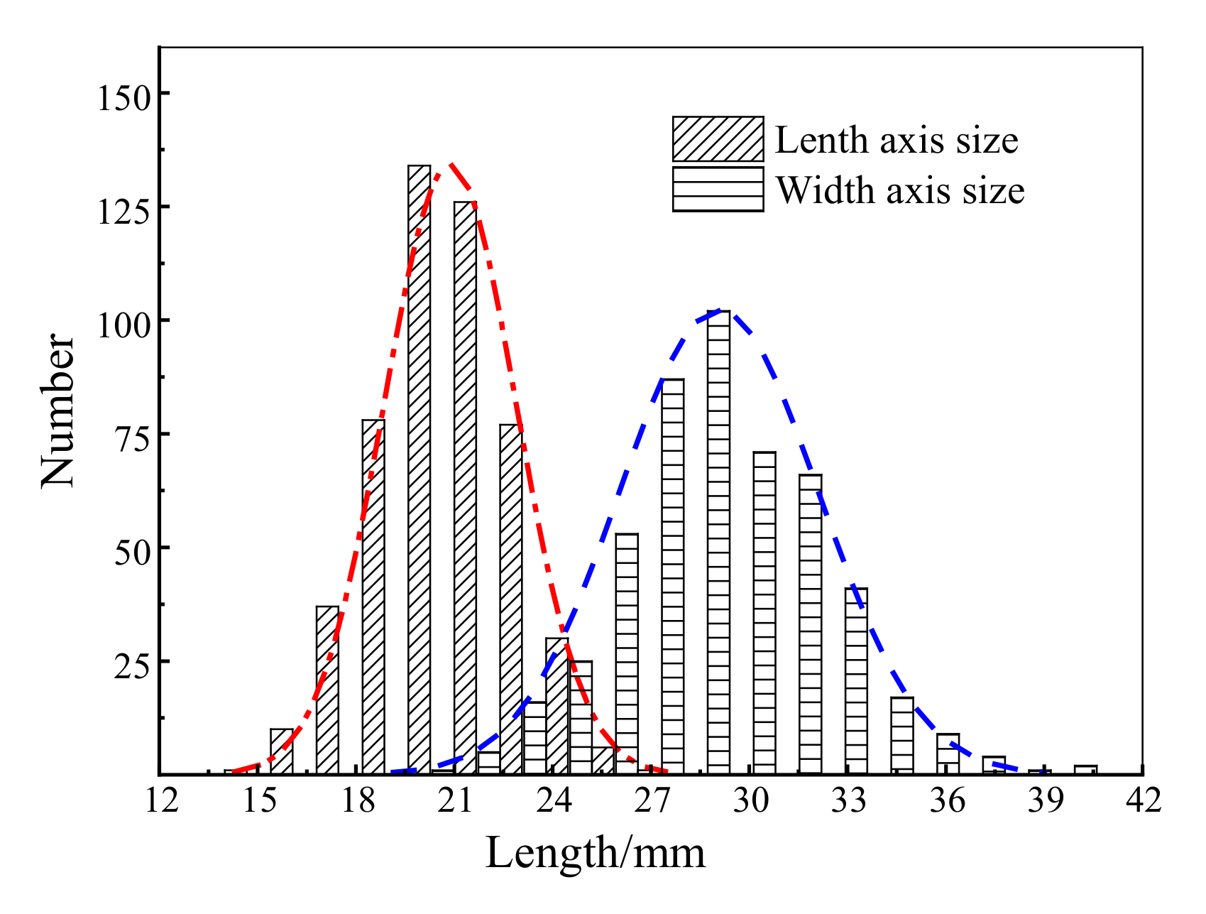
2.2.1. Size Distribution of FJF

A total of 500 FJF particles were randomly selected from the 10 kg samples to measure the length and width axis size with a digital display vernier caliper (measuring range: 150 mm; measuring accuracy: 0.02 mm), according to the method of Mahawar et al. [21], and the size distribution plotted in Figure 1.

2.2.2. Poisson’s Ratio and Shearing Modulus of FJF

The Poisson’s ratio and shear modulus of the FJF were measured by the uniaxial compression test method using a texture analyzer (UKTA-XT plus). A total of 50 FJF were randomly selected from the 10 kg of samples for the compression tests in the transverse and longitudinal directions. The diameter of the compression plate was 60 mm. The compression speed and loading displacement were set to 20 mm·min−1 and 20 mm. The compression test process was recorded with a high-speed camera. Then, the videos of size deformation of FJF were analyzed with FasMotion software, and the longitudinal and transverse deformations were obtained. The Poisson’s ratio and shear modulus of the FJF were calculated by Equations (1) and (2) [22].
ν = Δ ε x Δ ε y = Δ d x · d y Δ d y · d x
G = σ 2 Δ ε y 1 + ν
Note: v is the Poisson’s ratio; εx is the longitudinal strain (%); εy is the transverse strain (%); Δdy is the FJF longitudinal deformation (mm); dy is the original longitudinal size (mm); Δdx is the FJF transverse deformation, mm; dx is the original transverse original size (mm); G is the shear modulus (MPa); σ is the stress on the FJF (MPa).

2.3. Contact Parameters

The coefficient of restitution of FJF–FJF was measured by a method in which the FJF collides with a 45° inclined steel plate covered with closely arranged FJF. In the same way, the coefficient of restitution of the FJF–steel plate was measured by the collision of the FJF–steel plate with a 45° inclination. These methods were used by Wang et al. [23] and Feng et al. previously [24].
The static friction coefficient was measured by a cant instrument of a sloping platform with adjustable angles [25,26]. Three FJF samples stuck together were placed above the friction surface of the sloping platform; then, one end of the friction surface was raised gradually until the FJF just started to slide down. The tangent values of the angle between the friction surface and the horizontal plane were the static friction coefficient. The rolling friction coefficient was measured with the same method as the static friction coefficient; the difference was that only one FJF was used. The tangent values of the angle that the FJF started to roll was the sliding friction coefficient. The friction surface had two types: steel plate with FJF, and FJF with FJF. All of the above tests were repeated three times, and the results were calculated as an arithmetic average.

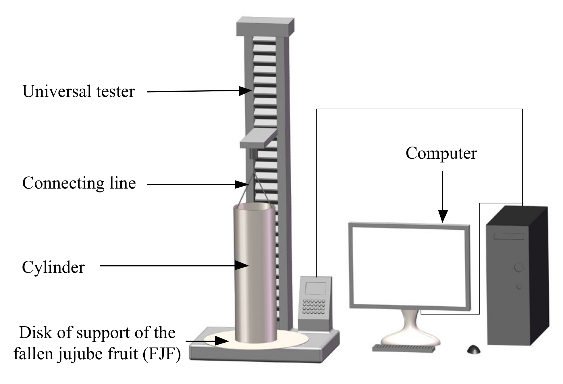
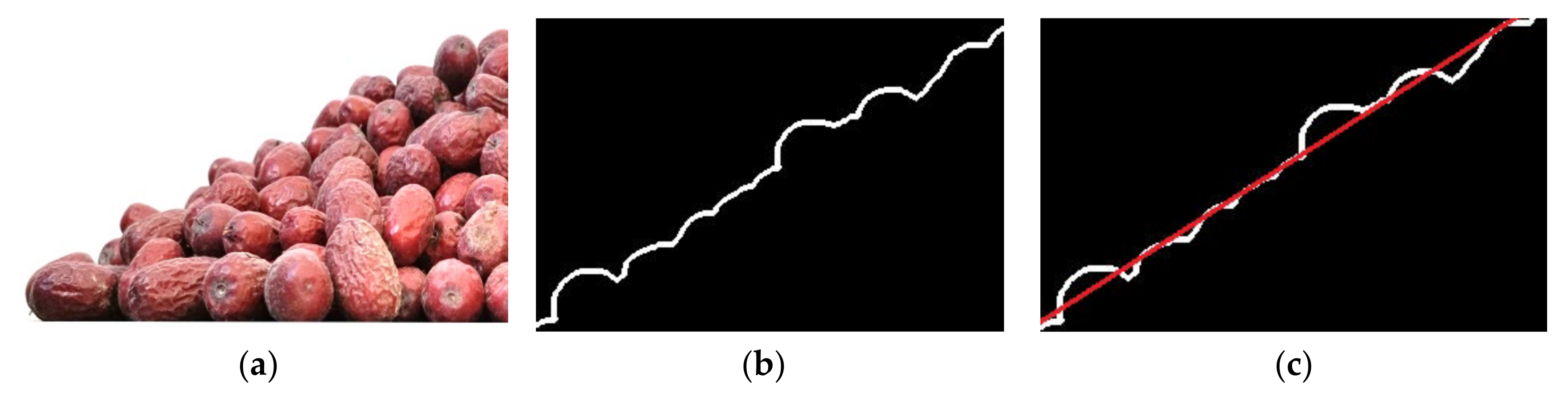
2.4. Angle of Repose Test

The cylinder lifting method was used to measure the angle of repose of FJF (Figure 2). During the test, the cylinder was placed vertically at the center of the disc of support of the FJF (450 mm in diameter) and the FJF were filled to the cylinder. A universal testing machine was used to lift the cylinder upward at a speed of 20 mm·s−1. The FJF naturally fell to accumulate and form a heap of FJF by the force of gravity. The angle between the FJF heap contour line and the disc was the angle of repose of the FJF.
The front-view image of the FJF heap was taken by a camera. The angle of repose was measured by the image processing method. Figure 3 is the image processing process of the angle of repose, and the values of the angle of repose were obtained by image segmentation (Figure 3a), boundary extraction (Figure 3b), and linear fitting (Figure 3c). To reduce the measurement errors, the same test was repeated three times, and two images were taken at 90° intervals in each group of tests. Bilateral values of each image were measured. The angle of repose of FJF was 29.85° and was obtained from an arithmetic average of the four results in each test.

2.5. EDEM Software Simulation Test

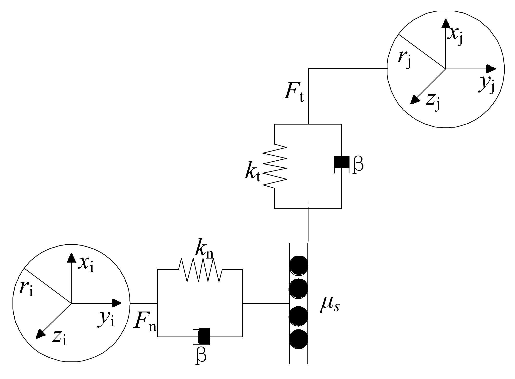
2.5.1. EDEM Software Simulation Principle

The FJF particles were large in size, smooth on the surface, and had no adhesion to each other, so the effects of surface energy were not considered [27]. Hence, the basic particle ball unit of the Hertz–Mindlin (no-slip) model in the EDEM software was selected to build the FJF simulation model. The normal force component was derived from the Hertzian contact theory [28], and the tangential component from work done by Mindlin [29]. Figure 4 is a schematic illustration of the Hertz–Mindlin contact model used in EDEM software.
The formulation of the normal force Fn is given by:
F n = 4 3 E * r * δ n 2 / 3
where δn is the normal overlap between contacting particles; E* is the equivalent Young’s modulus; and r* is equivalent particle radius; and their formulations are given by:
1 E * = 1 ν i 2 E i + 1 ν j 2 E j
1 r * = 1 r i + 1 r j
where Ei, Ej are the Young’s modulus of particle i and j; vi and vj are the Poisson’s ratio of particle i and j; ri, rj are the radius of particle i and j.
The formulation of the normal damping force F n d is given by:
F n d = 2 5 6 β k n m * v n r e l ¯
where v n r e l ¯ is the normal component of relative velocity; β is the effect of restitution; kn is the normal stiffness; m* is the equivalent mass; and their formulations are given by:
β = ln e ln 2 e + π 2
k n = 2 E * r * δ n
m * = 1 m i + 1 m j 1
where e is the coefficient of restitution, and mi, mj are the masses of particle i and j.
The formulation of the tangential force Ft is given by:
F t = S t σ t
k t = 8 G * r * δ n
where δt is the tangential overlap between contacting particles; kt is the tangential stiffness; G* is the equivalent shear modulus.
The formulation of the tangential damping F t d is given by:
F t d = 2 5 6 β k t m * v t r e l ¯
where v t r e l ¯ is the relative tangential velocity. The tangential force is limited by Mohr Coulomb friction behavior μsFn, where μs is the coefficient of static friction.
In this study rolling friction is applied by a torque to the contacting surface:
τ i = μ r F n R i ω i
where μr is the coefficient of rolling friction, Ri is the distance of the contact point from the center of mass, and ωi is the unit angular velocity of the object at the contact point.

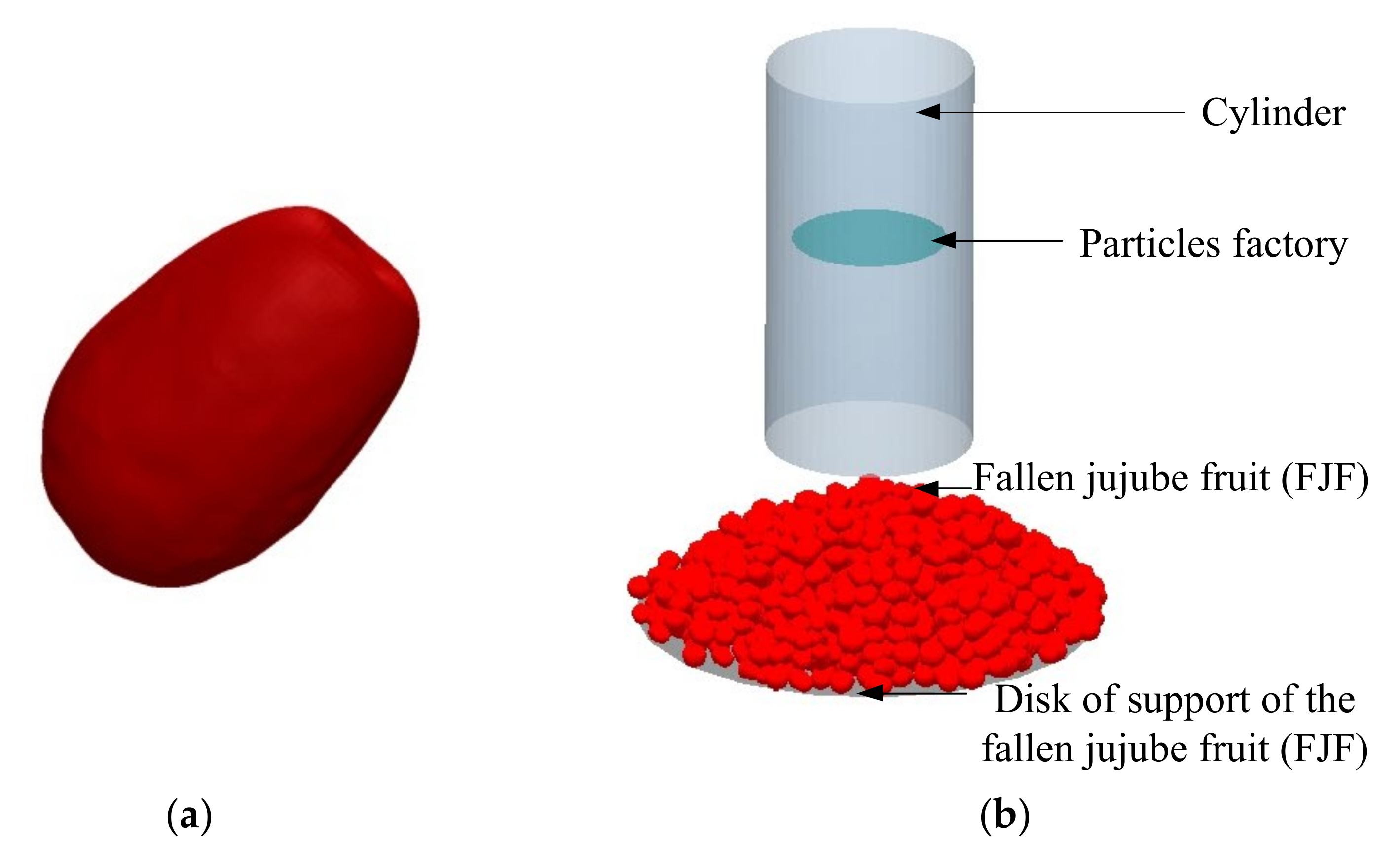
2.5.2. The Simulation Model of the Simulation Angle of Repose

The FJF 3D model was obtained by a 3D scanner (Figure 5a), and the FJF model was established by the round particle aggregation method in the EDEM 2018 software [30]. The simulation angle of repose experimental device was established by SolidWorks 2018 software (Dassault Systemes, Massachusetts, France), according to a 1:1 ratio with the physical test after simplifying the non-key components. Consequently, the FJF angle of repose simulation test model was obtained (Figure 5b). Depending on the pre-test, the jujube heap can be well formed when the number of FJF particles reaches 2000. Hence, the total number of generated FJF particles was set as 2000. The FJF particle generation rate, the fixed time step of the Rayleigh time step, and the data-saving interval time were set as 1000·s−1, 22%, and 0.01 s, respectively. Moreover, the grid size was set as three times the minimum spherical element size. The remaining simulation parameters were kept the same as the physical test.

2.5.3. Setting of Simulation Parameters

The characterization parameters and contact parameters are presented in Table 1 for the simulation tests. Among them, the density of the steel plate, Poisson’s ratio and shear modulus were obtained by referencing a machine design handbook [31]. The remaining parameters were obtained by physical tests.

2.6. Date Analysis

2.6.1. Plackett–Burman Experiment

The Plackett–Burman design method [32] was employed to encode the characterization parameters of FJF, the contact parameters of FJF–FJF, and the contact parameters of FJF–steel plate. The factors and levels are presented in Table 2.
The simulation angle of repose tests were carried out, and their values were measured according to the physical test measurement method. The pilot scheme and results with the Plackett–Burman design are displayed in Table 3.
The analysis module in the Design-Expert (Version 10.0.3) software was used to analyze the variance of the results, as shown in Table 4. The p values of the Poisson’s ratio A, static friction coefficient of FJF–FJF D, and static friction coefficient of FJF-steel plate G were both less than 0.05; these are the significant influence factors for influence of the simulation angle of repose.
Our study found that the significant factors affected by the simulation angle of repose are the Poisson’s ratio of FJF, static friction coefficient of FJF–FJF, and static friction coefficient of FJF–steel plate. However, Dai et al. [33] and Hou et al. [34] believed that the static friction coefficient, rolling friction coefficient, and coefficient of restitution of soil and agropyron seeds are the significant factors affecting the angle of repose. Moreover, Yuan et al. [15] reported that the coefficient of rolling friction, the contact model, and the coefficient of rolling friction of organic fertilizer–steel plate are the significant factors affecting the angle of repose. The reasons for this may be that the materials are extremely different in shape, volume, and characteristics, or that there were differences in the model parameter settings and simulation model establishment.

2.6.2. Steepest Ascent Search Experiment

A steepest ascent search experiment [35] was used to determine the optimal interval values of the significant influence factors. The level values were settled, increasing gradually according to the selected step. In addition, the remaining parameters were set at the intermediate level. The simulation angle of repose tests were carried out in accordance with the above setting parameters. The relative errors of the simulation and angle of repose were regarded as an experimental evaluation index. The arrangements and results of the steepest ascent search experiments are given in Table 5.
The simulation angle of repose values increased with the increase of the Poisson’s ratio of FJF A, the static friction coefficient of FJF–FJF D, and the static friction coefficient of FJF–steel plate G. However, the relative errors of simulation and the angle of repose initially decreased and then increased. The experimental evaluation index in group 2 had the smallest relative error of −5.12%. Therefore, the optimal parameter intervals were in group 1 and 3.

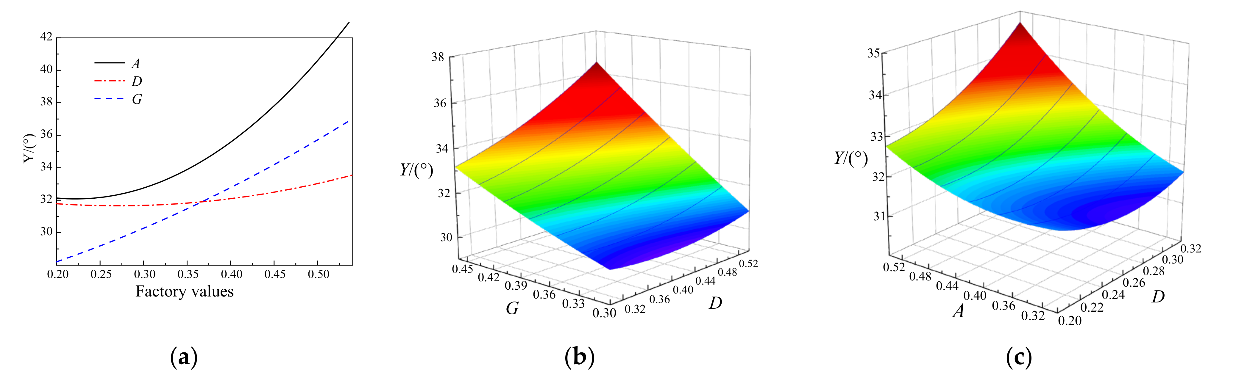
2.6.3. Central Composite Design Experiment

The Central Composite design experiment was employed to obtain accurate values for the significant influencing factors. Table 6 lists the encoding values of the significant influencing factors A, D, and G.
The simulation angle of repose value Y was regarded as the response evaluation index, and the significant influence factors A, D, and G were regarded as experimental factors. A three-factor and five-level central composite design experiment was designed. After that, the simulation test was carried out according to the experimental scheme. The experimental scheme and the results of the significant influencing factors are presented in Table 7.

3. Results and Discussion

3.1. Simulation Results

The analysis module of the Design-Expert (Version 10.0.3) software was utilized to process the experimental results. Table 8 shows the results of the regression variance analysis. The model’s coefficient (p ≤ 0.01) was extremely significant, and the lack of fit (p > 0.05) was non-significant. The coefficient of variation C.V. was 1.94%, which shows that the second-order response model reliability and the prediction value of the model fit with the physical test values. The second-order response model decision factor R2, correction decision factor R2adj, and prediction decision factor RPred were 0.955, 0.915, and 0.857, respectively. The signal-to-noise ratio was 20.41%, indicating the regression model is extremely significant. The results showed that the influencing factors A, D, and G have a high degree of interpretation of the response value Y. Furthermore, the second-order response model can predict and search for the best parameters of the simulation angle of repose under different conditions.
The p-values of factors D, G, and D × G were less than 0.01, which are extremely significant factors for the response value Y. The p-values of factors A, A × D, A × G, and A2 were 0.0153, 0.0421, 0.0081, and 0.0398, respectively, all in the range of 0.01 to 0.05, which are significant factors for the response value Y. The p-values of A × G, D2, and G2 were 0.4958, 0.0504, and 0.4236, respectively; these are all greater than 0.05, which indicates non-significant factors for the response value Y. The order affecting the response value Y is: G > D > D × G > A> A2 > A × D after ignoring the non-significant factors.
The second-order response model was obtained after excluding the nonsignificant affect factors on the angle of repose.
Y = 55.51 92.01 A 62.26 D 31.35 G + 72.79 A D + 77.25 D G + 110.06 A 2
Figure 6a shows the influence graphs of the experimental factors A, D, and G on Y (). The value of Y increases slowly when the value of A is between 0.2 to 0.3, and then Y increases rapidly from 33° to 42° when the value of A is greater than 0.3. Y does not vary significantly when the level value of D is between 0.2 and 0.4, and Y increases slowly with D when the level of D is greater than 0.4. In addition, with the increase of G, Y has an appropriately linear increase trend from 26° to 35°.
A response surface diagram was drawn to analyze the influence of interaction factors on the simulation angle of repose Y intuitively. Figure 6b shows the influence of interaction factors between static friction coefficient of FJF–FJF D and FJF–steel plate G on the simulation angle of repose Y. The influence of interaction factors between D and G had a significantly enhancing effect on the increase of Y. Y decreased initially, and then increased as D increased gradually when the value of G was less than 0.36. However, the value of Y increases slowly at first and then rapidly with the gradual increased of the value of D when G was greater than 0.36. The value of Y increased linearly with the increase of the value of G, and this trend became more obvious with the increase of D.
Figure 6c shows the influence of interaction factors between Poisson’s ratio A and the static friction coefficient of FJF–FJF D on the simulation angle of repose. Y decreases slowly initially and then increases gradually with the increase of the D when A is lower than 0.4. Y increases slowly firstly and then rapidly with the increase of the value of D when A is greater than 0.4. Y increases slightly with the increase of the A when the value of D is less than 0.24. Y increases slowly initially and then rapidly with the increase of A when the value of D is greater than 0.24.
With the angle of repose of FJF (29.85°) as a target, the optimization module in Design-Expert (Version 10.0.3) software was employed to search the optimized values from the regression equation. The minimum error between the angle of repose and simulation angle of repose was when Poisson’s ratio, static friction coefficient of FJF–FJF, and FJF–steel plate were 0.248, 0.480, and 0.309, respectively, which consequently were the optimal values.
There are diverse opinions regarding the laws of the simulation parameters on the angle of repose. In our study, the effect of the static friction coefficient between materials on the angle of repose was not obvious initially and then slowly increased, which agreed with the conclusion regarding the calibration of the contact parameters of chopped cotton straw conducted by Liang et al. [36]. However, Liu et al. [37] found that the static friction coefficient between particles has a linear variation trend with the angle of repose. In addition, Wu et al. [19] illustrated that the angle of repose increases significantly when the static friction coefficient values of corn seeds are less than 0.245, and the trend increases slowly when the value is greater than 0.245. Furthermore, Coetzee [38] reported that particle shapes have a marked effect on the angle of repose. For round particle materials, the angle of repose increases gradually with the increase of the static friction coefficient between particles. For materials consisting of several basic particle ball units, the angle of repose presents an irregular change trend with the change of the static friction coefficient between the particles. Consequently, the shape of the material may be a major reason for the abovementioned differences in research findings. There is a smaller contact area between the particles when the shape of the material is closer to a sphere. As a result, the effect of the static friction coefficient between particles on the angle of repose is more significant.

3.2. Verification Tests

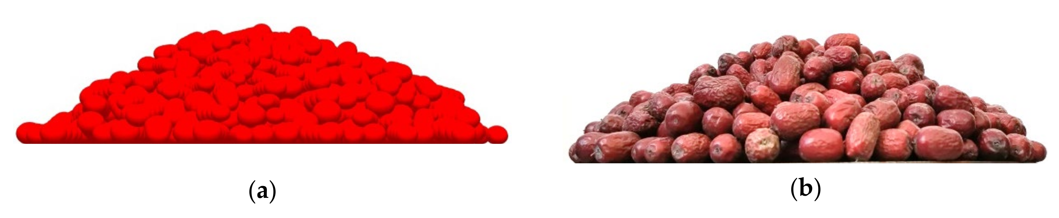
3.2.1. Angle of Repose Verification Tests

The accuracy of the simulation parameters was verified by comparing the error between the simulation and the physical angle of repose. In the verification simulation test, the significant influencing factors were set as the optimal values, and the remaining parameters were set at an intermediate level. Then, the simulation test of the angle of repose was conducted five times with EDEM 2018 software. The measured arithmetic average value was 29.69° (Figure 7a) of the simulated angle of repose, and the error (29.85°) (Figure 7b) was 0.53% compared to the angle of repose. The results indicated that the optimized experimental data are accurate and reliable, and that the calibrated simulation angle of repose model can represent the angle of repose tests.

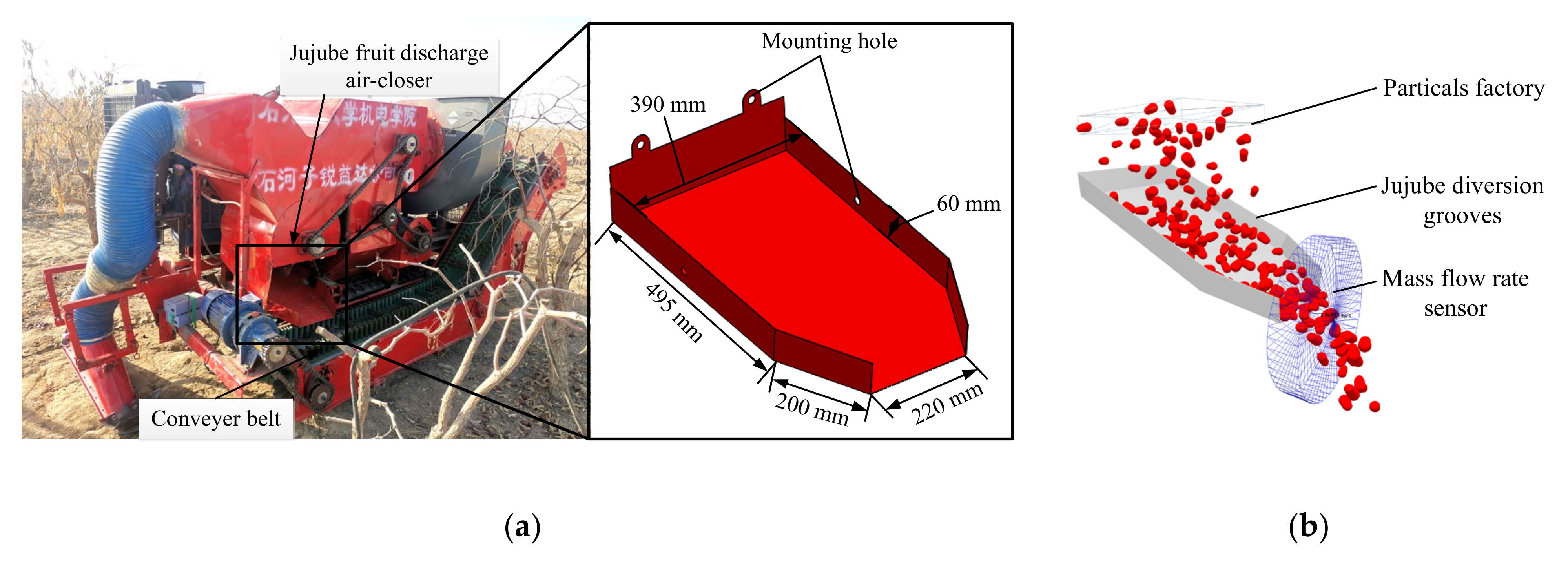
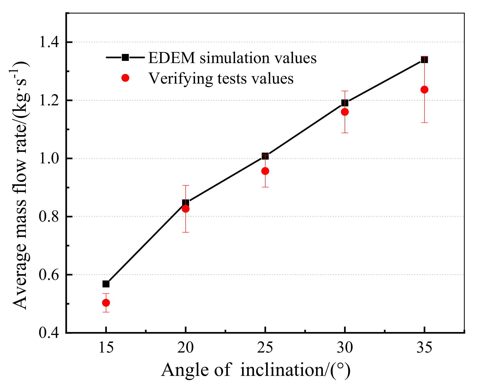
3.2.2. Verification Test of the Flow Rate of the FJF Guide Groove

The flow rate test was used to further verify the accuracy and applicability of the simulation parameters. The simulation test of the flow rate was performed by using the jujube guide groove of the air suction-picking jujube fruit harvester (Figure 8). The test results were compared with the physical test. The function of the guide groove is to transfer the FJF from the jujube fruit discharge air-closer to the conveyor belt. The incline of the guide groove is a significant factor affecting the flow rate. Figure 8a shows the placement and structure of the jujube guide groove.
The incline range of the jujube guide groove was set to vary from 15° to 35° in the simulation test, according to the actual operation situation. The parameters of the simulation model were input according to the above calibrated parameters, and the other test parameters were set in accordance with the actual operating parameters. The flow rate simulation test process of the FJF guide groove is presented in Figure 8b. The physical flow rate tests of the FJF guide groove were carried out in the same conditions as the simulation model. The results of the simulation tests and physical tests are shown in Figure 9. The average error of the flow rate between the physical and simulation tests was 5.84%. In addition, the maximum and minimum errors were 11.38% and 2.40%, which appeared at 15° and 20° incline angles, respectively. The test results indicated that the established EDEM simulation model with optimal parameters can guide the structural design of physical-mechanical devices.

4. Conclusions

The main purpose of this study was to obtain the simulation parameters of fallen jujube fruit (FJF) in DEM. The interval values of FJF’s intrinsic and contact parameters and the angle of repose were measured by physical tests. According to data processing methods, the simulation angles of the repose tests were carried out to obtain the specific simulation parameters from the interval values of the intrinsic and contact parameters. The results showed that the significant influencing factors were the Poisson’s ratio, the static friction coefficient of FJF–FJF, and the static friction coefficient of FJF–steel plate. The angle of repose verification tests illustrated that the error was 0.53% between the simulated angle of repose (29.69°) and the angle of repose (29.85°). Furthermore, the flow rate verification tests found that the average error was 5.84%, and the maximum and minimum errors were 11.38% and 2.40%, respectively. This demonstrated that the calibrated FJF simulation parameters are accurate and reliable. This study can provide a simulation model for FJF for developing machinery and equipment through the EDEM simulation method. In the future, it will be interesting to conduct more tests to verify the accuracy of the established model, so that it can apply to broader fields.

Author Contributions

Conceptualization, methodology, data curation, formal analysis, writing—original draft, writing—review and editing, G.S. and J.L.; investigation, H.D.; data curation, L.D.; funding acquisition, J.L.; validation, Z.Z.; software, N.L.; supervision, Z.K. All authors have read and agreed to the published version of the manuscript.

Funding

This research was funded by the Regional Innovation Guidance Plan of the XPCC (Xinjiang Production and Construction Corps), grant number: 2021BB003.

Institutional Review Board Statement

Not applicable.

Informed Consent Statement

Not applicable.

Data Availability Statement

The data presented in this study are available on request from the corresponding author.

Conflicts of Interest

The authors declare no conflict of interest.

References

  1. Li, J.W.; Fan, L.P.; Ding, S.D.; Ding, X.L. Nutritional composition of five cultivars of Chinese jujube. Food Chem. 2007, 103, 454–460. [Google Scholar] [CrossRef]
  2. National Statistics Bureau of the People’s Republic of China. China Statistical Yearbook; China Statistics Press: Beijing, China, 2020. [Google Scholar]
  3. Hu, Y.S.; Bai, B.W.; Wang, W. Present Development Situation of Red Jujube Industry in Xinjiang and Relative Countermeasures and Suggeation. Xinjiang Agric. Mech. 2016, 6, 21–24. [Google Scholar]
  4. Al-Niami, J.H.; Saggar, R.; Abbas, M.F. The physiology of ripening of jujube fruit (Zizyphus spina-christi (L.) Willd.). Sci. Hortic. 1992, 51, 303–308. [Google Scholar] [CrossRef]
  5. Lu, H.F.; Lou, H.Q.; Zheng, H.; Hu, Y.; Li, Y. Nondestructive Evaluation of Quality Changes and the Optimum Time for Harvesting During Jujube (Zizyphus jujuba Mill. cv. Changhong) Fruits Development. Food Bioprocess Technol. 2012, 5, 2586–2595. [Google Scholar] [CrossRef]
  6. Coetzee, C.J. Review: Calibration of the discrete element method. Powder Technol. 2017, 310, 104–142. [Google Scholar] [CrossRef]
  7. Michael, R.; Hanley, K.J. A methodical calibration procedure for discrete element models. Powder Technol. 2017, 307, 73–83. [Google Scholar]
  8. Chen, Z.P.; Wassgren, C.; Veikle, E.; Ambrose, K. Determination of material and interaction properties of maize and wheat kernels for DEM simulation. Biosyst. Eng. 2020, 195, 208–226. [Google Scholar] [CrossRef]
  9. Han, D.D.; Zhang, D.X.; Jing, H.R.; Yang, L.; Cui, T.; Ding, Y.Q.; Wang, Z.D.; Wang, Y.X.; Zhang, T.L. DEM-CFD coupling simulation and optimization of an inside-filling air-blowing maize precision seed-metering device. Comput. Electron. Agric. 2018, 150, 426–438. [Google Scholar] [CrossRef]
  10. Zeng, Z.W.; Ma, X.; Chen, Y.; Qi, L. Modelling residue incorporation of selected chisel ploughing tools using the discrete element method (DEM). Soil Tillage Res. 2020, 197, 104505. [Google Scholar] [CrossRef]
  11. Zhang, S.; Tekeste, M.Z.; Li, Y.; Gaul, A.; Zhu, D.; Liao, J. Scaled-up rice grain modelling for DEM calibration and the validation of hopper flow. Biosyst. Eng. 2020, 194, 196–212. [Google Scholar] [CrossRef]
  12. Zhao, L.L.; Zhao, Y.M.; Bao, C.Y.; Hou, Q.F.; Yu, A.B. Optimization of a circularly vibrating screen based on DEM simulation and Taguchi orthogonal experimental design. Powder Technol. 2017, 310, 307–317. [Google Scholar] [CrossRef]
  13. Wang, G.Q.; Hao, W.J.; Wang, J.J. Discrete Element Method and Practice on EDEM; Northwestern Polytechnical University Press: Xi’an, China, 2010. [Google Scholar]
  14. Wen, B.; Li, Y.; Kan, Z.; Li, J.B.; Li, L.Q.; Ge, J.B.; Ding, L.P.; Wang, K.F.; Zou, S.J.; Li, W.T. Experimental Research on the Bending Characteristics of Glycyrrhiza glabra Stems. Trans. ASABE 2020, 63, 1–10. [Google Scholar] [CrossRef]
  15. Yuan, Q.C.; Xu, L.M.; Xing, J.J.; Duan, Z.Z.; Ma, S.; Yu, C.C.; Chen, C. Parameter calibration of discrete element model of organic fertilizer particles for mechanical fertilization. Trans. Chin. Soc. Agric. Eng. 2018, 34, 21–27. [Google Scholar]
  16. Wen, X.Y.; Yuan, H.F.; Wang, G.; Jia, H.L. Calibration Method of Friction Coefficient of Granular Fertilizer by Discrete Element Simulation. Trans. Chin. Soc. Agric. Mach. 2020, 51, 115–122. [Google Scholar]
  17. Wang, Y.X.; Liang, Z.J.; Zhang, D.X.; Cui, T.; Shi, S.; Li, K.R.; Tan, G.L. Calibration method of contact characteristic parameters for corn seeds based on EDEM. Trans. Chin. Soc. Agric. Eng. 2016, 32, 36–42. [Google Scholar]
  18. Wang, W.W.; Cai, D.Y.; Xie, J.J.; Zhang, C.L.; Liu, L.C.; Chen, L.Q. Parameters Calibration of Discrete Element Model for Corn Stalk Powder Compression Simulation. Trans. Chin. Soc. Agric. Mach. 2021, 52, 127–134. [Google Scholar]
  19. Wu, M.C.; Cong, J.L.; Yan, Q.; Zhu, T.; Peng, X.Y.; Wang, Y.S. Calibration and experiments for discrete element simulation parameters of peanut seed particles. Trans. Chin. Soc. Agric. Eng. 2020, 36, 30–38. [Google Scholar]
  20. Razavi, S.; Pourfarzad, A.; Sourky, A.H.; Jahromy, S. The Physical Properties of Fig (Ficus carica L.) as a Function of Moisture Content and Variety. Philipp. Agric. Sci. 2010, 93, 170–181. [Google Scholar]
  21. Mahawar, M.K.; Bibwe, B.; Jalgaonkar, K.; Ghodki, B.M. Mass modeling of kinnow mandarin based on some physical attributes. J. Food Process Eng. 2019, 42, 1–11. [Google Scholar] [CrossRef]
  22. Artiukh, V.; Mazur, V.; Sagirov, Y.; Larionovet, A. New Methods for Determining Poisson’s Ratio of Elastomers. In Energy Management of Municipal Transportation Facilities and Transport; Springer: Cham, Switzerland, 2019; pp. 71–80. [Google Scholar]
  23. Wang, C.J.; Li, Y.M.; Ma, L.Z.; Ma, Z. Experimental study on measurement of restitution coefficient of wheat seeds in collision models. Trans. Chin. Soc. Agric. Eng. 2012, 28, 274–278. [Google Scholar]
  24. Feng, B.; Sun, W.; Shi, L.R.; Sun, B.G.; Zhang, T.; Wu, J.M. Determination of restitution coefficient of potato tubers collision in harvest and analysis of its influence factors. Trans. Chin. Soc. Agric. Eng. 2017, 33, 50–57. [Google Scholar]
  25. Liu, W.Z.; He, J.; Li, H.W.; Li, X.Q. Calibration of Simulation Parameters for Potato Minituber Based on EDEM. Trans. Chin. Soc. Agric. Mach. 2018, 49, 125–135. [Google Scholar]
  26. Shi, L.R.; Ma, Z.T.; Zhao, W.Y.; Yang, X.P.; Sun, B.G.; Zhang, J.P. Calibration of simulation parameters of flaxed seeds using discrete element method and verification of seed-metering experiment. Trans. Chin. Soc. Agric. Eng. 2019, 35, 25–33. [Google Scholar]
  27. Paulick, M.; Morgeneyer, M.; Kwade, A. Review on the influence of elastic particle properties on DEM simulation results. Powder Technol. 2015, 283, 66–76. [Google Scholar] [CrossRef]
  28. Hertz, H. On the contact of elastic solids. Journal für die reine und angewandte Mathematik. Crelles J. 1882, 92, 156–171. [Google Scholar]
  29. Mindlin, R.D. Compliance of Elastic Bodies in Contact. J. Appl. Mech. 1949, 16, 259–268. [Google Scholar] [CrossRef]
  30. Ma, Z.; Li, Y.M.; Xu, L.Z. Discrete-element method simulation of agricultural particles’ motion in variable-amplitude screen box. Comput. Electron. Agric. 2015, 118, 92–99. [Google Scholar] [CrossRef]
  31. Wen, B.C. Machine Design Handbook; Machinery Industry Press: Beijing, China, 2010; Volume 5. [Google Scholar]
  32. El-Sheekh, M.M.; Khairy, H.M.; Gheda, S.F.; El-Shenody, R.A. Application of Plackett-Burman design for the high production of some valuable metabolites in marine alga Nannochloropsis oculata. Egypt. J. Aquat. Res. 2016, 42, 57–64. [Google Scholar] [CrossRef] [Green Version]
  33. Dai, F.; Song, X.F.; Zhao, W.Y.; Zhang, F.W.; Ma, H.J.; Ma, M.Y. Simulative calibration on contact parameters of discrete elements for covering soil on whole plastic film mulching on double ridges. Trans. Chin. Soc. Agric. Mach. 2019, 50, 49–56. [Google Scholar]
  34. Hou, Z.F.; Dai, N.Z.; Chen, Z.; Qiu, Y.; Zhang, X.W. Measurement and calibration of physical property parameters for Agropyron seeds in a discrete element simulation. Trans. Chin. Soc. Agric. Eng. 2020, 36, 46–54. [Google Scholar]
  35. Horabik, J.; Wiacek, J.; Parafiniuk, P.; Banda, M.; Kobylka, R.; Stasiak, M.; Molenda, M. Calibration of discrete-element-method model parameters of bulk wheat for storage. Biosyst. Eng. 2020, 200, 298–314. [Google Scholar] [CrossRef]
  36. Liang, R.Q.; Chen, X.G.; Jiang, P.; Zhang, B.C.; Meng, H.W.; Peng, X.B.; Kan, Z. Calibration of the simulation parameters of the particulate materials in film mixed materials. Int. J. Agric. Biol. Eng. 2020, 13, 29–36. [Google Scholar] [CrossRef]
  37. Liu, C.L.; Wei, D.; Song, J.N.; Du, X.; Zhang, F.Y. Systematic Study on Boundary Parameters of Discrete Element Simulation of Granular Fertilizer. Trans. Chin. Soc. Agric. Eng. 2018, 49, 82–89. [Google Scholar]
  38. Coetzee, C.J. Calibration of the discrete element method and the effect of particle shape. Powder Technol. 2016, 297, 50–70. [Google Scholar] [CrossRef]
Figure 1. The length and width axis size distribution of 500 fallen jujube fruit (FJF).
Agriculture 12 00038 g001
Figure 2. The angle of repose test device for the cylinder lifting method.
Agriculture 12 00038 g002
Figure 3. The angle of repose of the fallen jujube fruit (FJF) image processing steps; (a) image segmentation, (b) boundary extraction, and (c) linear fitting of the boundary curve.
Agriculture 12 00038 g003
Figure 4. The schematic illustration of the Hertz–Mindlin (no-slip) contact model used in EDEM software.
Agriculture 12 00038 g004
Figure 5. The simulation model and simulation angle of repose test; (a) 3D model of fallen jujube fruit (FJF) obtained by three-dimensional scanning, (b) test process of the simulation angle of repose.
Agriculture 12 00038 g005
Figure 6. The influence of single factors and interaction factors on the simulation angle of repose; (a) single factors, (b) static friction coefficient between fallen jujube fruit (FJF) D and fallen jujube fruit (FJF)–steel plate G, and (c) Poisson’s ratio of fallen jujube fruit (FJF) A and static friction coefficient between fallen jujube fruit (FJF) D.
Agriculture 12 00038 g006
Figure 7. The angle of repose results; (a) simulation test angle of repose, (b) physical test angle of repose.
Agriculture 12 00038 g007
Figure 8. The flow rate simulation tests of fallen jujube fruit (FJF) using the jujube guide groove; (a) placement and structural dimensions of the FJF guide groove, (b) simulation tests of the flow rate.
Agriculture 12 00038 g008
Figure 9. The physics and simulation test results of the flow rate were carried out using the fallen jujube fruit (FJF) guide groove.
Agriculture 12 00038 g009
Table 1. The simulation parameters and their values for the fallen jujube fruit (FJF) and steel plate.
ParamentsValues
Solids density/kg·m−3fallen jujube fruit (FJF)807.87 ex
steel plate7850 re 31
Poisson’s ratiofallen jujube fruit (FJF)0.2–0.5 ex
steel plate0.3 re 31
Shear Modulus/MPafallen jujube fruit (FJF)0.03–0.9 ex
steel plate7.94 re 31
Fallen jujube fruit (FJF)–fallen jujube fruit (FJF)coefficient of restitution0.1–0.4 ex
static friction coefficient0.3–0.9 ex
rolling friction coefficient0.03–0.06 ex
Fallen jujube fruit (FJF)–steel platecoefficient of restitution0.2–0.5 ex
static friction coefficient0.3–0.7 ex
rolling friction coefficient0.02–0.05 ex
Note: ex represents the values obtained by the physical test. re represents the values obtained by referring to a machine design handbook.
Table 2. The factors and levels of the simulation parameters for the Plackett–Burman design.
FactorsLevels
−10+1
A: Poisson’s ratio of fallen jujube fruit (FJF)0.20.350.5
B: Shear modulus of fallen jujube fruit (FJF)0.030.4650.9
C: Coefficient of restitution between fallen jujube fruit (FJF)0.10.250.4
D: Static friction coefficient between fallen jujube fruit (FJF)0.30.60.9
E: Rolling friction coefficient between fallen jujube fruit (FJF)0.030.0450.06
F: Coefficient of restitution between fallen jujube fruit (FJF)–steel plate0.20.350.5
G: Static friction coefficient between fallen jujube fruit (FJF)–steel plate0.30.50.7
H: Rolling friction coefficient between fallen jujube fruit (FJF)–steel plate0.020.0350.05
Table 3. The schemes and results of the simulation parameters with the Plackett-Burman design.
No.ABCDEFGHIJKAngle of Repose (°)
10.50.90.40.30.030.20.70.0211−133.56
20.20.90.40.90.030.20.30.05−11132.24
30.20.90.40.30.060.50.70.02−1−1135.76
40.20.90.10.90.060.20.70.051−1−139.54
50.50.90.10.90.060.50.30.02−11−132.78
60.50.030.40.90.030.50.70.05−1−1−135.26
70.20.030.40.30.060.50.30.0511−128.87
80.20.030.10.30.030.20.30.02−1−1−127.61
90.50.030.40.90.060.20.30.021−1132.77
100.20.030.10.90.030.50.70.0211140.71
110.50.030.10.30.060.20.70.05−11132.14
120.50.90.10.30.030.50.30.051−1125.68
130.350.4650.250.60.0450.350.50.03500039.57
Table 4. The variance analysis results of the Plackett–Burman Design with the analysis module in the Design-Expert (Version 10.0.3) software.
Source of VarianceSum of SquaresDegrees of FreedomMean SquareF-Valuep-Value
Model212.43826.5521.320.014 *
A13.07113.0710.490.048 *
B0.4010.400.320.61 NS
C0.0010.000.000.999 NS
D73.38173.3858.910.0046 **
E3.8313.833.070.178 NS
F0.1210.120.100.777 NS
G114.181114.1891.650.002 **
H7.4517.455.980.092 NS
Curvature38.86138.8631.190.011 *
Residual3.7431.25
Cor total255.0312
Note: ** denotes the extremely significant influence factors (p ≤ 0.01); * denotes the significant influence factors (0.01 < p ≤ 0.05); NS denotes the non-significant influence factors (p > 0.05).
Table 5. The arrangements and results of significant influencing factors (Poisson’s ratio of FJF A, static friction coefficient of FJF–FJF D, and static friction coefficient of FJF–steel plate G) with a steepest ascent search experiment.
No.Experimental FactorsSimulation Angle of Repose/(°)Relative Errors/%
ADG
10.20.30.326.7214.58%
20.260.420.3832.26−5.12%
30.320.540.4634.50−11.28%
40.380.660.5436.67−16.53%
50.440.780.6238.12−19.70%
60.50.90.740.55−24.50%
Table 6. The encoding values of the significant influencing factors (the Poisson’s ratio of FJF A, the static friction coefficient of FJF–FJF D and the static friction coefficient of FJF–steel plate G) with a central composite design.
LevelsADG
−1.680.160.220.25
−10.20.30.3
00.260.420.38
10.320.540.46
1.680.360.620.51
Table 7. The experimental schemes and the results of the significant influencing factors (the Poisson’s ratio of FJF A, the static friction coefficient of FJF–FJF D, and the static friction coefficient of FJF–steel plate G) with the central composite design.
No.CodingResponse ValuesNo.CodingResponse Values
ADGYADGY
1−1−1−136.30 ± 0.38110−1.68030.89 ± 1.06
21−1−133.04 ± 2.111201.68034.85 ± 1.77
3−11−129.25 ± 2.241300−1.6829.96 ± 1.04
411−138.05 ± 1.2214001.6830.47 ± 2.67
5−1−1132.31 ± 1.971500033.96 ± 0.92
61−1132.68 ± 3.611600032.93 ± 1.76
7−11135.74 ± 0.691700032.41 ± 1.91
811133.92 ± 1.071800031.48 ± 1.47
9−1.680032.01 ± 0.961900031.50 ± 0.96
101.680033.48 ± 1.842000031.93 ± 2.19
Table 8. The regression variance analysis of the significant influencing factors (the Poisson’s ratio of FJF A, the static friction coefficient of FJF–FJF D, and the static friction coefficient of FJF–steel plate G) by the analysis module.
SourceSum of SquaresdfF-ValueMean Squarep-Value
Model86.6199.6223.75<0.0001 **
A3.4513.458.520.0153 *
D11.86111.8629.280.0003 **
G60.55160.55149.43<0.0001 **
A × D2.2012.205.420.0421 *
A × G0.2010.200.500.4958
D × G4.4014.4010.860.0081 **
A22.2612.265.580.0398 *
D22.0012.004.940.0504
G20.2810.280.700.4236
Residual4.05100.41
Lack of Fit1.0950.220.370.8528
Pure error2.9750.59
Cor total90.6719
R2 = 0.955; R2adj = 0.915; C.V = 1.94%; R2Pred = 0.857
Note: ** denotes the extremely significant factors (p ≤ 0.01); * denotes the significant factors (0.01< p ≤0.05); NS means the non-significant factors (p > 0.05).
Publisher’s Note: MDPI stays neutral with regard to jurisdictional claims in published maps and institutional affiliations.

