Multi-Feature Optimization Study of Soil Total Nitrogen Content Detection Based on Thermal Cracking and Artificial Olfactory System

Abstract

To improve the accuracy of detecting soil total nitrogen (STN) content by an artificial olfactory system, this paper proposes a multi-feature optimization method for soil total nitrogen content based on an artificial olfactory system. Ten different metal–oxide semiconductor gas sensors were selected to form a sensor array to collect soil gas and generate response curves. Additionally, six features such as the response area, maximum value, average differential coefficient, standard deviation value, average value, and 15th-second transient value of each sensor response curve were extracted to construct an artificial olfactory feature space (10 × 6). Moreover, the relationship between feature space and soil total nitrogen content was used to establish backpropagation neural network (BPNN), extreme learning machine (ELM), and partial least squares regression (PLSR) models were used, and the coefficient of determination (R²), root mean square error (RMSE), and the ratio of performance to deviation (RPD) were selected as prediction performance indicators. The Monte Carlo cross-validation (MCCV) and K-means improved leave-one-out cross-validation (K-means LOOCV) were adopted to identify and remove abnormal samples in the feature space and establish the BPNN model, respectively. There were significant improvements before and after comparing the two rejection methods, among which the MCCV rejection method was superior, where values for R², RMSE, and RPD were 0.75671, 0.33517, and 1.7938, respectively. After removing the abnormal samples, the soil samples were then subjected to feature-optimized dimensionality reduction using principal component analysis (PCA) and genetic algorithm-based optimization backpropagation neural network (GA-BP). The test results showed that after feature optimization the model indicators performed better than those of the unoptimized model, and the PLSR model with GA-BP for feature optimization had the best prediction effect, with an R² value of 0.93848, RPD value of 3.5666, and RMSE value of 0.16857 in the test set. R² and RPD values improved by 14.01% and 50.60%, respectively, compared with those before optimization, and RMSE value decreased by 45.16%, which effectively improved the accuracy of the artificial olfactory system in detecting soil total nitrogen content and could achieve more accurate quantitative prediction of soil total nitrogen content.

1. Introduction

The sum of the various forms of nitrogen in the soil is called soil total nitrogen (STN). For arable soils, fertilization systems, crop rotations and utilization patterns all have a strong influence on the total soil nitrogen content. Moreover, it is an essential indicator for maintaining crop yield and plays a vital role in crop development and agroecosystems [1,2,3]. In precision agriculture, obtaining information on dynamic changes is important to improve nitrogen fertilizer utilization and cropping patterns [4,5]. Therefore, it is of significance to improve the accuracy of measuring soil total nitrogen content and to obtain information on soil total nitrogen more rapidly and accurately [6].

Kjeldahl and Dumas combustion methods are the classical methods for the determination of total soil nitrogen, which have high measurement accuracy but are time-consuming and laborious, and the chemical reagents used are prone to secondary contamination. Elemental analyzers based on the Dumas combustion method are fast, but expensive, require high-precision analytical balances, and the copper powder normally required for the reduction reaction is environmentally hazardous. In recent years, soil total nitrogen detection methods based on remote sensing technology and spectral analysis have received attention from many scholars because of their advantages of being non-destructive, accurate, and efficient. Zhang et al. [7] used the CASI-1500 aerial hyperspectral imaging system to capture soil spectral information and three models to predict total nitrogen values in black soils, demonstrating that hyperspectral remote sensing is an efficient method for soil nutrient content estimation. Li et al. [8] applied hyperspectral techniques to extract characteristic wavelengths using an uninformative variable elimination algorithm (UVE) and successive projection algorithm (SPA), and then combined partial least squares (PLS) and extreme learning machine (ELM) to build a soil total nitrogen prediction model, achieving better prediction results. Although these methods compensate for the shortcomings of classical methods to a certain extent, the high cost of analytical instruments, the influence of the atmosphere, and iron–oxide in the soil severely limit their application [9].

Thermal cracking can crack large molecule compounds into volatile small-molecule gas compounds, and using gas sensor arrays to obtain cracking gas information, the artificial olfactory system can achieve detection of soil total nitrogen content. This method has the advantages of being convenient, fast, and inexpensive, while the gas sensors are inexpensive and reusable. However, redundant samples and dimensional disasters reduce machine learning efficiency, pattern recognition accuracy, and data mining efficiency, and increase the workload of experiments to some extent [10]. Shi et al. [11] used various methods to reject abnormal samples for NIR light detection to improve the model prediction performance; Ji Ma et al. [12] studied the introduction of principal component analysis algorithm for dimensionality reduction to reduce the difficulty of deep learning in extracting image features and verified its feasibility with simulation experiments. Xu K et al. [13] used mean analysis, coefficient of variation analysis, cluster analysis and correlation analysis to obtain the feature matrix of the optimized electronic nose to detect hickory, and PLSR and backpropagation neural network (BPNN) to build a regression model to obtain evidence that the optimized method improved the performance of the electronic nose and reduced the dimensionality of the data. Vung Pham et al. [14] proposed an interactive visualization method for portable X-ray fluorescence (pXRF) data analysis of soil profiles and innovated a model RDNet to achieve accurate results for predicting $p{H}_{H_{2}O}$ and $p{H}_{KCl}$. Antonios Morellos et al. [15] compared the predictive performance of two linear multivariate methods (principal component regression and partial least squares regression) and two machine learning methods (least squares support vector machines and Cubist) for total soil nitrogen, organic carbon, and moisture, based on near-infrared spectral data collected from 140 soil samples. For purposes of solving the above problems, this paper explores the performance improvement of a thermal cracking and manual olfactory system-based method for the determination of total soil nitrogen, using coefficient of determination (R²), root mean square error (RMSE), and the ratio of performance to deviation (RPD) as measures in the test set. The first stage of optimization (abnormal sample rejection) was to identify abnormal samples in the dataset by comparing the Monte Carlo cross-validation (MCCV) method with the K-means improved leave-one-out cross-validation (K-means LOOCV) method. The better rejection method is selected by comparing the performance of the BPNN model before and after the rejection of these abnormal samples. In the second stage of optimization (feature dimensionality reduction), soil olfaction spatial dimensionality reduction was performed using principal component analysis (PCA) and genetic algorithm-based optimization backpropagation neural network (GA-BP) methods, and BPNN, ELM, and partial least squares (PLSR) were established. The experimental results showed the method proposed in this study (MCCV + GA-BP) could effectively improve the performance index of the artificial olfaction system for detecting STN.

2. Materials and Methods

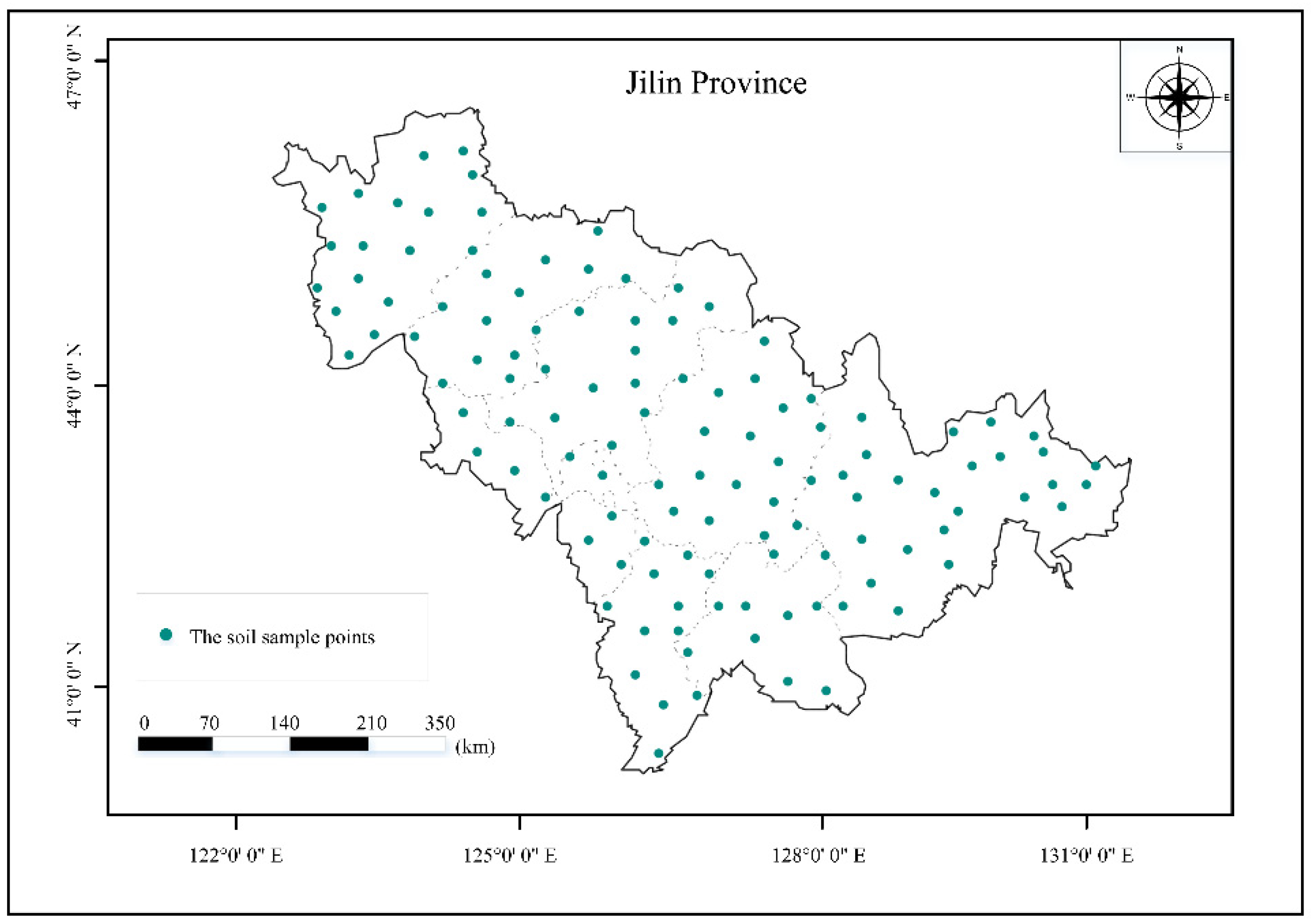
2.1. Study Area and Soil Samples

The study area is located in northeastern China, as shown in Figure 1 (44°50′ N, 121°38′ E, 46°19′ N, 131°19′ E), with a sampling area of 187,400 km², in a temperate continental monsoon climate with an average annual temperature of 5.1 °C, average annual rainfall of 400–600 mm, and one of the world’s three prime maize belts, which is an important grain-producing area. It is one of the most important grain-producing regions in China. The main soil types in the region include dark brown loam, black calcium soil, white pulp soil, herbaceous soil, and black soil, and is one of the major production areas of maize and rice in China. Due to the crop rotation pattern and improper fertilization, the total nitrogen content of the soil has decreased, thus this study aims to help optimize fertilization to improve the soil nutrient content structure and protect the black soil.

Soil sampling was conducted from 1 September to 20 October 2020. Based on the land-use status, topographic features, etc., and considering the principles of randomness and representativeness, a total of 121 sampling points were selected, as shown in Figure 1. The latitude and longitude information of the sampling points were recorded by GPS, and soil was collected at a depth of 0–20 cm with a soil extractor [16], and stones, plant debris, and roots were removed from the soil. The collected samples were placed in self-sealing bags and brought back to the laboratory for processing. The samples were divided into two parts, one part used the Kjeldahl method to measure the STN content in the soil, where the samples were then naturally dried at 25 °C, crushed, placed through a 0.2 mm nylon sieve to filter out impurities, bagged and set aside. The whole nitrogen content was obtained as the actual value by this method. The other part was used for measuring STN content with an artificial olfactory system, and no special treatment was required for the samples.

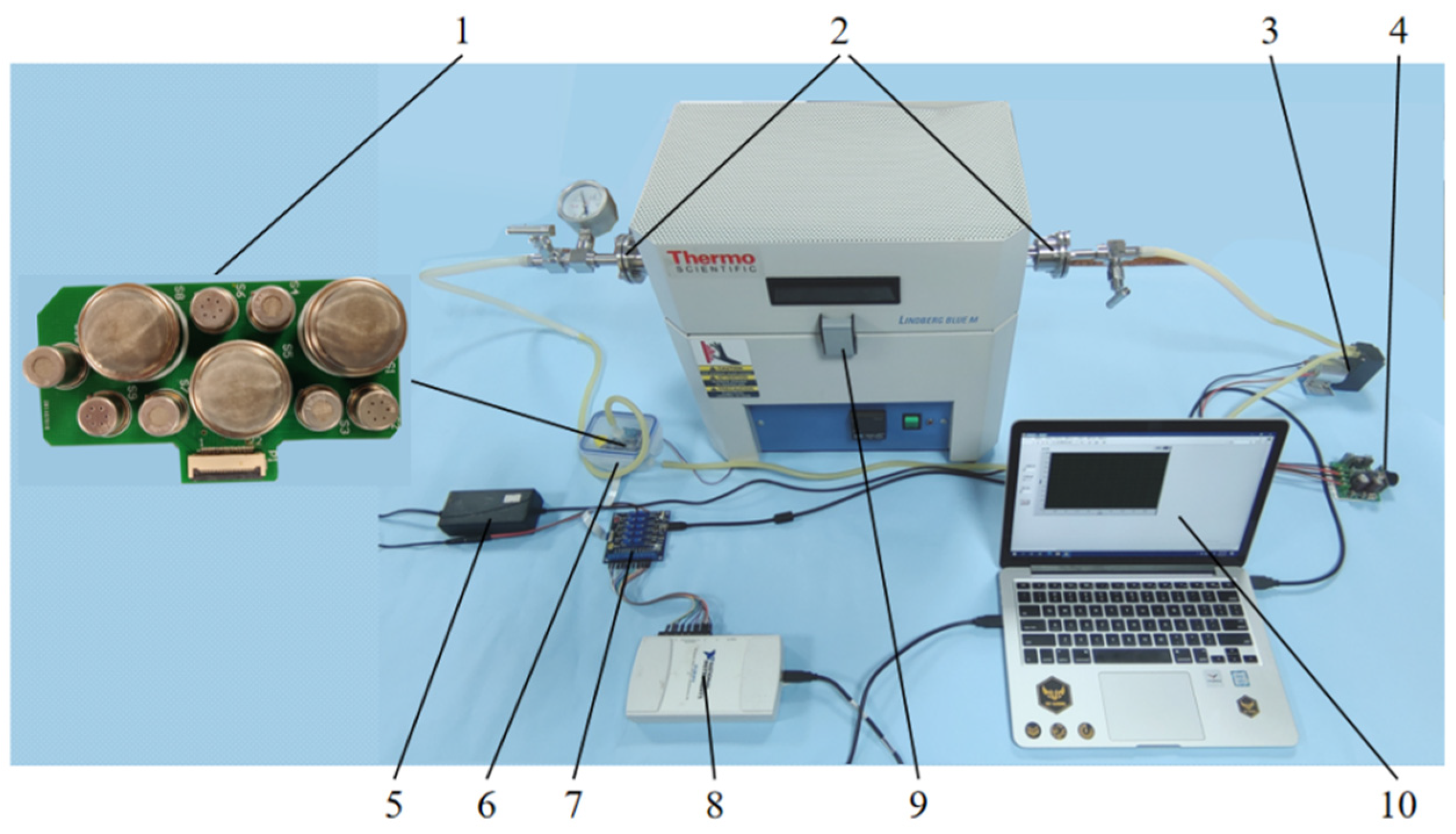
2.2. Research on Artificial Olfactory System

The artificial olfactory system is divided into three main parts [17]. In the first part, sample preparation; in the second part, detection system; and in the third part, data processing system. Figure 2 shows the hardware components of the detection system which mainly includes the muffle furnace, gas sensor array, reaction chamber, valve, gas pump (for cleaning the reaction chamber), signal processing module, data acquisition card, and computer. The muffle furnace, manufactured by Thermo Scientific Lindberg, USA, is used here for cracking large molecular compounds in soil. The gas sensor array is located in the reaction chamber and communicates with the signal processing module through the flexible flat cable (FFC). The data acquisition card connects to the signal processing module through a DuPont cable and transfers the acquired data to the computer via USB for display and storage. Power is supplied to the signal processing module by a 12 V power adapter. Among them, the gas sensor array is the basis of the detection system, as shown in

Table 1. Sensor Type Table.

Sensor Type	Detection of Gas Types	Measurement Range
TGS826	Ammonia	30–300 ppm
TGS2602	Toluene, ammonia, hydrogen sulfide	1–30 ppm
TGS2610	Tropane, butane	500–10,000 ppm
TGS2620	Ethanol, organic solvent	50–5000 ppm
TGS821	Hydrogen	100–1000 ppm
TGS2603	Trimethylamine, methyl mercaptan, etc.	1–10 ppm
TGS2611	Methane, natural gas	500–10,000 ppm
TGS823	Methane, ethanol vapor	50–300 ppm
TGS2600	Hydrogen, alcohol, etc.	1–30 ppm
TGS2612	methane, propane, isobutane	3000–9000 ppm

, this study uses MOS sensors produced by Figaro Japan specifically for high-precision detection of low concentration gases. This sensor array has a high specificity and some cross-sensitivity, which improves the accuracy compared to a single type of sensor array. The signal processing module is used to power the sensor array and the measurement circuit output. A USB-6210 acquisition card from National Instruments (NI) was used to acquire the gas sensor array response data.

Upon starting the system, 3 g of soil sample was weighed with an electronic scale and placed inside a quartz boat, which was placed in the middle of the quartz tube and sealed with vacuum flanges at both ends. The lysis temperature and time were 450 °C and 2 min, respectively [18]. First, the flanges on both sides were opened and the vacuum pump fed completed soil gas from the cracking into the response chamber while the detection started. The sampling time was 80 s, and the sensor array converted the soil gas information into a voltage signal through a signal processing circuit to generate a soil sample response curve. After the test was completed, the air chamber was cleaned with 1200 mL·min⁻¹ clean air, quartz boat and quartz tube were washed with water, and the two sampling intervals were 5 min. The test was completed sequentially according to the soil sample number.

2.3. Feature Extraction

The obtained ten response curves of soil samples were first processed by Savitzky-Golay convolution filtering to extract six characteristic values of response area ($V_{RAV}$), mean differential coefficient ($V_{MDC}$), standard deviation value ($V_{SDV}$), mean value ($V_{MV}$) maximum value ($V_{MAX}$), and 15th s transient value ($V_{15TH}$) on the sensor response curve. There was a total of 60 features per soil sample. Since the different magnitudes of the data are not conducive to model building, the z-score method was chosen to complete the standardization of the data. $V_{RAV}$, $V_{MDC}$, $V_{SDC}$, $V_{MV}$ were defined as follows:

$$V_{RAV}={\displaystyle {\sum }_{i=1}^N{X}_i}\Delta t$$

(1)

$$V_{MDC}=\frac{1}{N-1}{\displaystyle {\sum }_{i=1}^{N-1}\frac{X_{\mathrm{i}+1}-X_{\mathrm{i}}}{\Delta t}}$$

(2)

$$V_{SDV}=\sqrt{\frac{{{\displaystyle {\sum }_{i=1}^N\left(X_i-V_{MV}\right)}}^2}{N}}$$

(3)

$$V_{MV}=\frac{{\displaystyle {\sum }_{i=1}^N{X}_i}}{N}$$

(4)

where X_i is the i-th data collected by the sensor, Δt is the time interval between 2 adjacent sampling points, taken as 0.1 s, and N the total number of collected data.

2.4. Training Set and Test Set Division

For purposes of finding the optimal adjustment parameters, preventing the phenomenon of “overfitting”, and improving the generalization ability of the model, the data set was randomly divided according to the Kennard-Stone method in the ratio of 7:3, i.e., the training set was 85 and the test set was 36.

Table 2. Organic matter concentrations in soil samples.

Dataset	STN (g kg−1)	Mean Values (g kg−1)	Variance (g kg−1)
Training set	1.42, 1.65, 1.81, 1.39, 1.38, 1.75, 1.17, 1.25, 0.84, 1.46, 1.38, 1.80, 1.64, 1.27, 1.33, 0.20, 1.85, 1.5, 2.18, 1.90, 2.38, 0.52, 1.29, 0.36, 1.35, 2.18, 1.15, 0.93, 2.02, 0.35, 1.51, 2.14, 1.73, 1.56, 1.32, 1.66, 1.57, 1.40, 1.34, 1.18, 0.68, 1.26, 1.14, 0.92, 0.64, 1.09, 1.83, 0.72, 1.52, 1.24, 1.93, 1.76, 2.12, 1.94, 1.92, 0.47, 1.69, 1.97, 0.95, 1.22, 1.84, 2.33, 2.13, 1.08, 2.35, 4.10, 1.47, 0.78, 1.07, 2.03, 2.31, 1.28, 2.37, 1.78, 1.70, 1.10, 1.53, 2.79, 3.95, 3.75, 1.41, 3.07, 1.30, 1.20, 0.46	1.56	0.51
Test set	1.95, 1.98, 1.16, 3.57, 1.53, 1.45, 3.98, 0.98, 2.44, 1.06, 0.94, 0.90, 1.52, 1.23, 1.68, 2.22, 0.91, 1.37, 2.17, 1.21, 1.96, 0.69, 1.54, 0.85, 1.48, 1.30, 1.40, 0.53, 2.39, 1.34, 2.59, 1.60, 0.96, 2.95, 1.31, 2.16	1.64	0.60

illustrates the statistical results of the STN content of the samples measured by the Kjeldahl method. The variance and mean values were 0.60 $\mathrm{g}·{\mathrm{kg}}^{-1}$ and 1.64 $\mathrm{g}·{\mathrm{kg}}^{-1}$ for the test set and 0.51 $\mathrm{g}·{\mathrm{kg}}^{-1}$ and 1.56 $\mathrm{g}·{\mathrm{kg}}^{-1}$ for the verification set, respectively, which can be approximated to show there is no significant difference between the two.

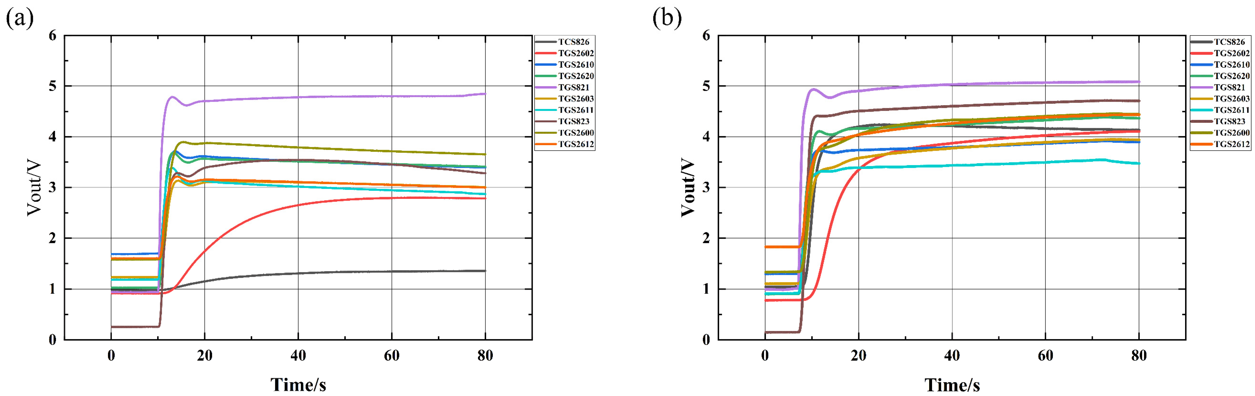
2.5. Sensor Array for Full Nitrogen Feature Space Response

In sequence to verify whether the sensor array composition was reasonable, fracking gas data were selected with a whole nitrogen content of 0.2 mg·kg⁻¹ and 4.10 mg·kg⁻¹, respectively, and Figure 3 was obtained. As shown in the figure, each sensor showed a large difference in response to different soil gases simultaneously, indicating that the array has good sensitivity to the difference in fracking gases. The response results indicate that the selected sensor array is reasonable.

2.6. Multi-Feature Optimization Methods and Pattern Recognition Prediction Models

2.6.1. Abnormal Sample Removal Method

The main reasons for generating abnormal samples are the design error of the artificial olfactory system itself, complexity of the samples, and instability of the instrument state [19]. In the modeling process, these abnormal samples heavily interfere with the prediction performance of the model, thus this study explores MCCV and K-means LOOCV to discriminate and remove abnormal samples of the system, respectively, and aims to obtain the best abnormal sample removal method for the detection method of the artificial olfactory system according to the comparison of the performance prediction index of the processed BPNN model.

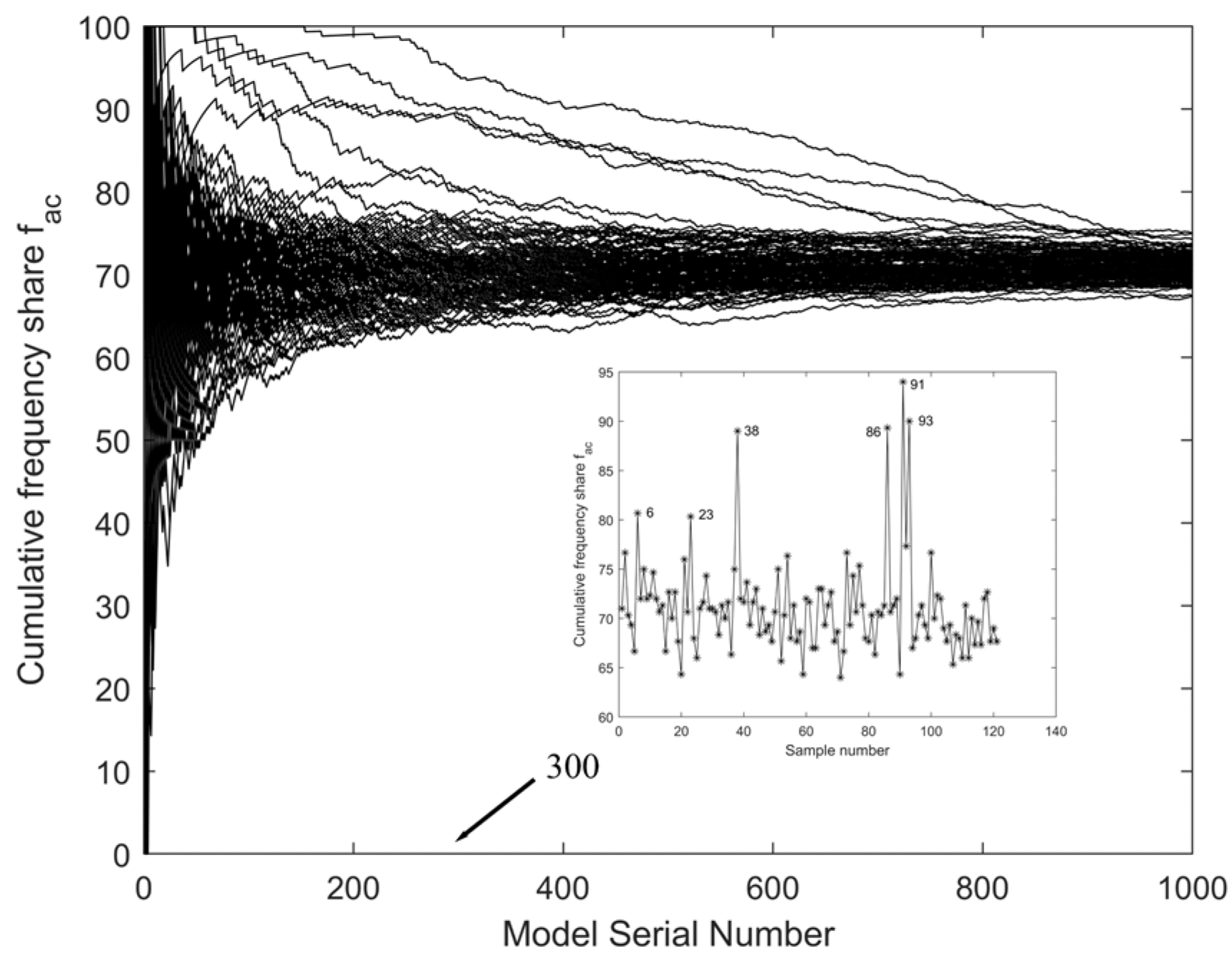
2.6.2. Monte Carlo Cross Validation Method

Monte Carlo cross-validation (MCCV) is a hypothesis-based method [20,21]. In this study, the MCCV method is used to discriminate abnormal samples in the olfactory feature space. Firstly, 70% of samples are randomly selected on the training set for the construction of BPNN models, and the remaining 30% are predicted; then the above process is repeated to construct multiple BPNN models; finally, each model is ranked in ascending order according to the sum of squared residuals (PRESS) of the test set, and the cumulative probability ($f_{ac}$) to determine abnormal samples. The definitions of PRESS and fac are as follows:

$$PRESS={\displaystyle {\sum }_{i=1}^k{({\widehat{y}}_i-y_i)}^2}$$

(5)

$$f_{ac}\left(m,n\right)=100\times {\displaystyle {\sum }_{n=1}^N{{\displaystyle f}}_{mn}}/121$$

(6)

where (5) equation k is the number of predicted samples, ${\widehat{y}}_i$ and $y_i$ represent the predicted and observed values of the i-th sample; (6) equation m is the sample ordinal number and n is the sorted model ordinal number, $f_{mn}$ indicates whether sample m appears in the calibration set of model n, and is 1 if it appears, and 0 otherwise, N represents the total number of samples (121 in this study).

By definition, the change of $f_{ac}$ with model ordinal number will reflect the probability of each sample in the model, since the model has been sorted by PRESS value. As the model ordinal number increases, the normal $f_{ac}$ will remain at about 70% of the sampling rate, and conversely, the abnormal sample will deviate from the normal sample.

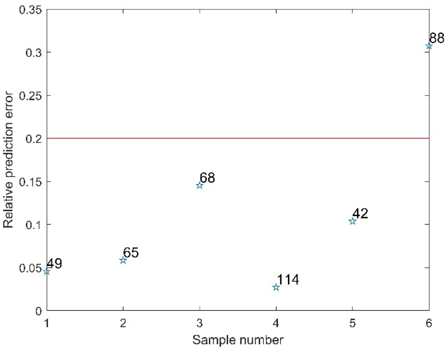
2.6.3. K-Means LOOCV Cross Validation

Leave-one-out cross-validation (LOOCV) treats each sample as an abnormal sample and obtains a prediction model with the same number of samples by training modeling one by one, which is a computationally intensive process [22]. K-means LOOCV is perfection of LOOCV in abnormal sample identification which is time-consuming and has the deficiency of misclassification. The olfactory space is clustered based on the K-means clustering method, and the number of clusters is set. Subsequently, the test set is screened, and based on the principle that normal samples are more concentrated while abnormal samples are more discrete, the classes with fewer samples in the clustering are taken as suspicious abnormal samples. To construct the prediction model, the remaining samples with the suspicious abnormal samples removed are used as the training set, and a BPNN prediction model is trained with this. The LOOCV step is then bridged to reduce the time to train the model. The steps of the K-means LOOCV method are as follows:

(1)

Spatial clustering of soil olfaction based on K-means clustering with a set number of clusters.

(2)

The classes with fewer samples in the clustering are treated as suspect samples and used as the test set for the BPNN model.

(3)

The remaining samples with suspected anomalies removed are taken as the training set and used to train a BPNN prediction model.

(4)

The input prediction of the test set with the trained model gives the corresponding prediction results and the relative error δ between the predicted and measured values is calculated.

(5)

Set the threshold value. If the value is greater than the threshold, it is considered an abnormal sample, otherwise it is considered a normal sample.

2.7. Feature Dimensionality Reduction Methods

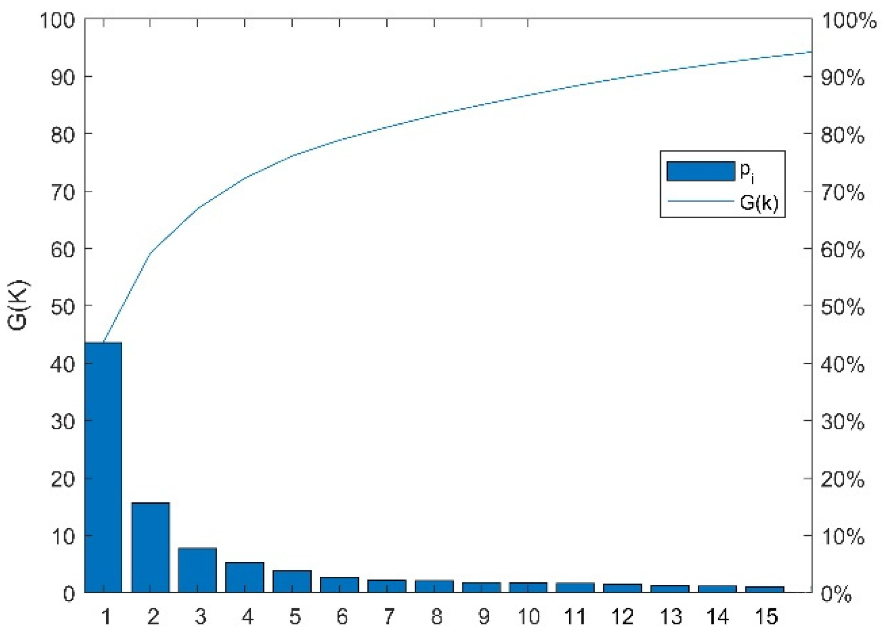
2.7.1. Principal Component Analysis

Principal component analysis (PCA) is a mathematical dimensionality reduction method [23,24,25,26]. The covariance matrix of the olfactory space is first calculated, followed by finding the eigenvalues of the covariance matrix and their corresponding eigenvectors, and ranking the eigenvectors according to the magnitude of the eigenvalues to obtain the eigenvector matrix; the first k (1 ≤ k < 60) vectors of the eigenvector matrix are selected, and the original olfactory space is reduced to k dimensions. The selection of its k can be determined by the cumulative contribution of variance information G(k) in Equation (8). As in Equation (7), let the variance contribution rate be $p_i$ and ${\gamma }_j$ denote the i-th (i < k) and j-th (j < 60) sorted eigenvalues, respectively.

$$p_i={\gamma }_i/{\displaystyle {\sum }_j^{60}{\gamma }_j}$$

(7)

$$G\left(k\right)={\displaystyle {\sum }_{i=1}^k{p}_i}$$

(8)

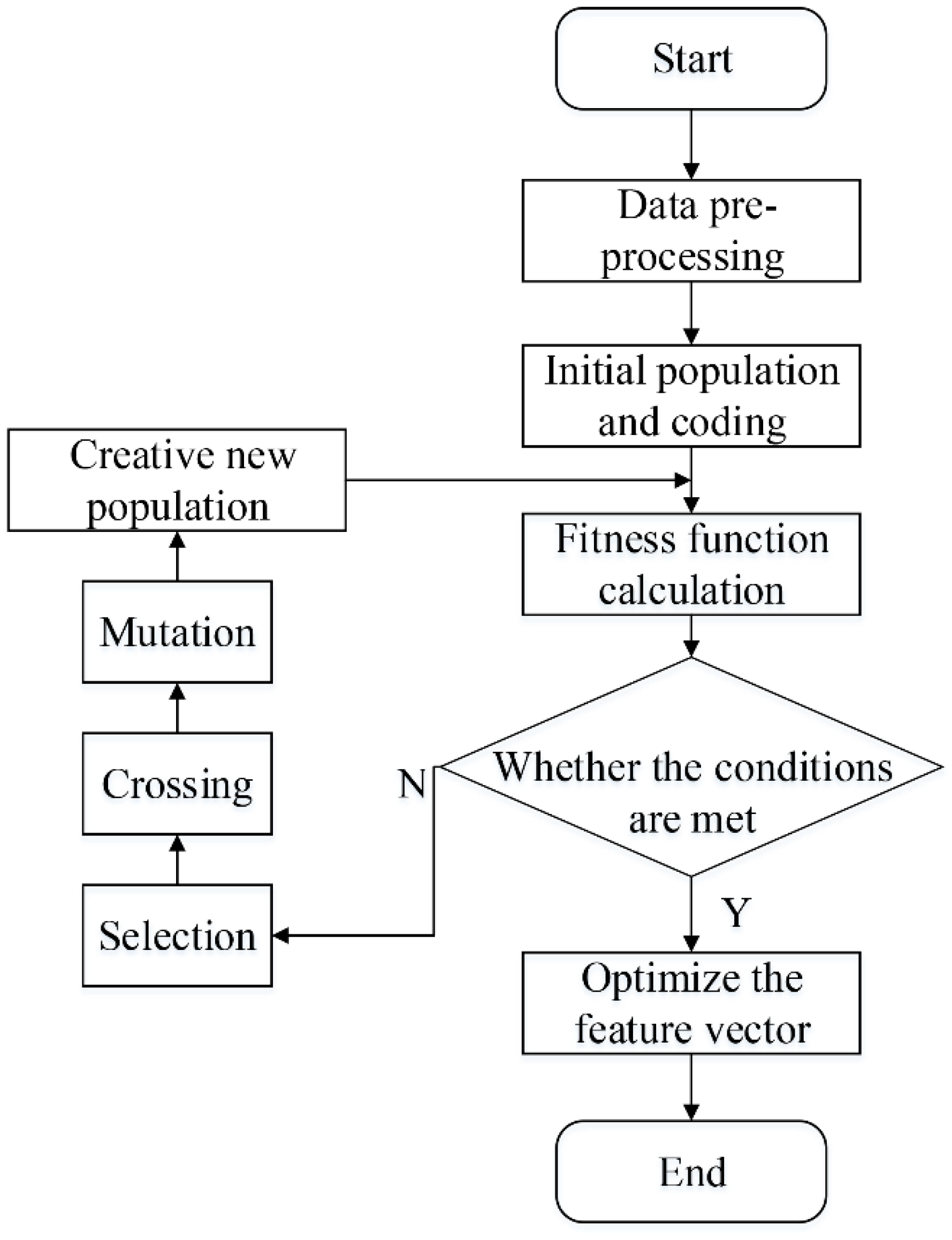
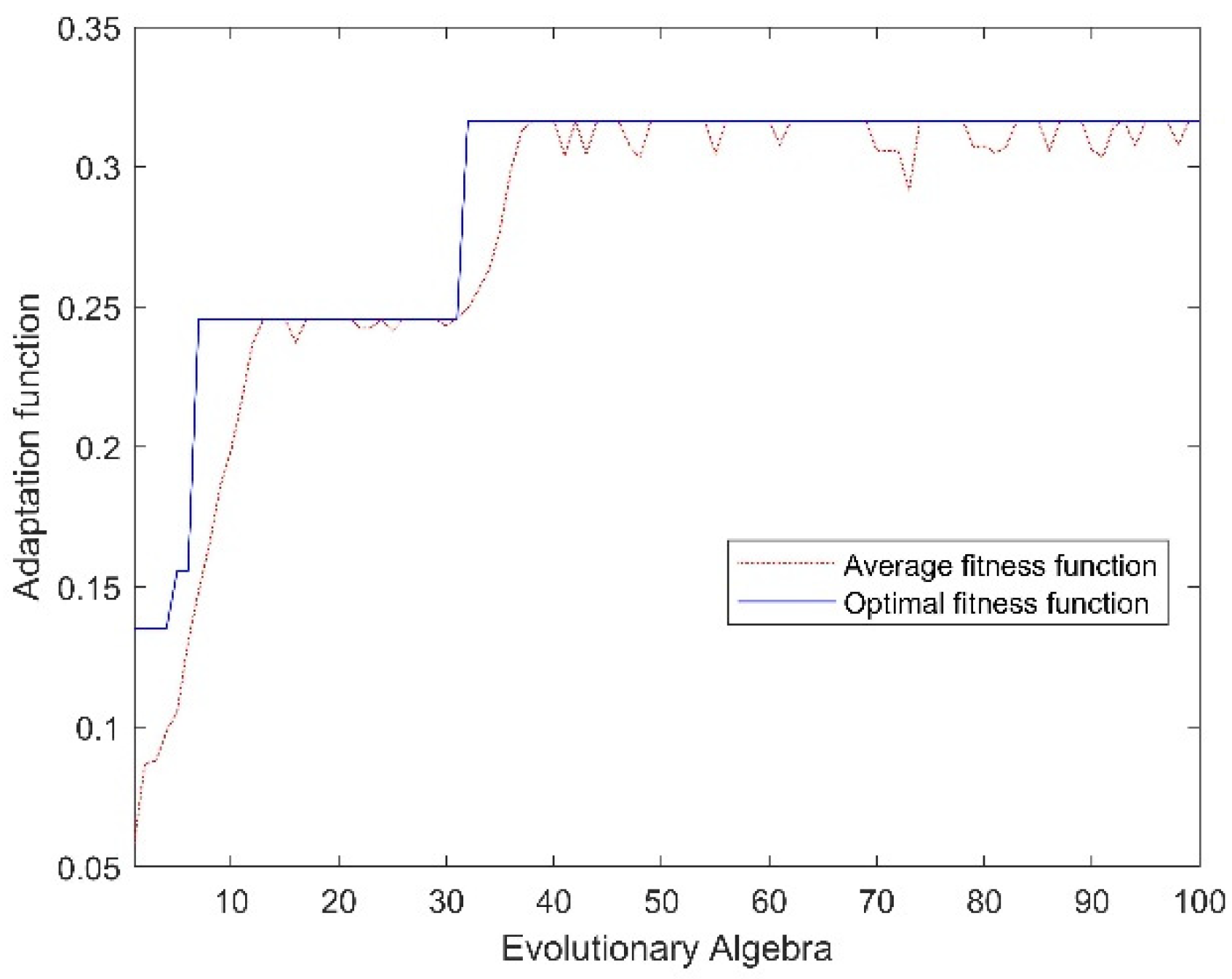
2.7.2. GA-BP Optimization

In order to ensure the validity of soil olfactory feature space information to a greater extent, the genetic algorithm-backpropagation neural network (GA-BP) optimization method is used in soil total nitrogen detection. The process is shown in Figure 4. A total of 30 samples are randomly selected to form a population, the dimension of the original olfactory space is 60 in line with the chromosome coding length, the coding is binary, and a feature vector corresponds to one gene on the chromosome. If the value of the gene is 1, it will participate in BPNN modeling, and vice versa, if the gene is 0, the feature vector will not participate in modeling. The feature vector corresponding to the genetic individual is selected to build the BPNN model, and the model is trained with the data in the training set, and the inverse of the sum of squares of the errors in the test set data is used as the fitness function. Assuming g(x) is the fitness function, ${\widehat{y}}_i$ is the predicted value of the BPNN model for the i-th sample in the test set, and $y_i$ is the observed value of the i-th sample in the test set, then it can be expressed as follows:

$$g(x)=\frac{1}{{\displaystyle {\sum }_{i=1}^n{\left({\widehat{y}}_i-y_i\right)}^2}}$$

(9)

First determine whether the parameters of the feature vector satisfy the losing condition. If it satisfies then output the preferred feature vector and end the run; otherwise, perform the operations of genetic algorithm such as selection, crossover, mutation, and generation of new populations [27,28], and then repeat the above steps until the output condition is satisfied.

2.8. Pattern Recognition Prediction Model for Artificial Olfactory System

2.8.1. BPNN Prediction Algorithm

Backpropagation neural network (BPNN) belongs to multilayer feedforward neural networks, which have the advantages of simple structure and strong nonlinear mapping capability [29,30]. According to Kolmogorov theory, a three-layer network containing one hidden layer can approximate any nonlinear function [31]. This paper is based on the neural network toolbox in MATLAB (2019a) software, which is a mathematical software produced by MathWorks, based in Natick, MA, USA. The BPNN is first created by selecting the linear transfer function as the output layer function and the logarithmic transfer function as the hidden layer function. The number of nodes H in the hidden layer is too large or too small for the model. The approximate range can be obtained from the empirical Equation (10), and the optimal number of hidden layers can be obtained by combining the modeling metrics. The BPNN created to predict the total nitrogen content of the soil was trained for 1000 iterations with a learning rate of 0.001 and a convergence condition of 0.00004. The optimal number of implicit layer nodes for direct modelling was determined to be 8 based on the number of model input and output nodes and the RMSE.

$$H=\sqrt{m+n}+\alpha$$

(10)

where $\alpha$ is the regulation constant between 1 and 10, and m and n are the number of input and output nodes, respectively.

2.8.2. ELM Prediction Model

Extreme learning machine (ELM) is a special feedforward neural network developed on the basis of single implicit layer feedforward neural network [32]. Unlike the traditional feedforward neural network based on the gradient descent method, the modeling process randomly generates the connection weights between the input layer and the hidden layer and the thresholds of the neurons in the hidden layer, and there is no necessity to adjust the training process, only the number of hidden nodes needs to be set, which transforms the problem of finding the optimal solution into a simple least-squares problem, which is not easy to fall into the local minima and has good generalization ability. The selection of the implicit function must be integrated with the prediction correctness of the test set to make an appropriate choice. The elmtrain function is used to create and train the ELM model. TYPE in the function is selected as 0, indicating regression fitting, the activation function is selected as sigmoid, and the elmpredict function is used for the predicted output of the model, which is set to be consistent with the elmtrain parameters.

2.8.3. PLSR Prediction Model

Partial least squares regression (PLSR) is a regression modeling method of multiple dependent variables on multiple independent variables in which the regression process is built by extracting the principal components of the dependent and independent variables as much as possible and by maximizing the correlation between the principal components extracted from them, respectively [33]. In the modeling process, linear regression models are constructed by finding predictor variables and observable variables in a new space instead of finding the hyperplane of maximum variance between the response and independent variables. PLSR extracts the principal components from the variables to reduce the predictor variable covariance of the sample while addressing the problem of excess predictor variables.

2.8.4. Model Evaluation Metrics

Given objective evaluation of the advantages and disadvantages of various pretreatment methods, this study compares before and after treatment and for which model optimization is better, the R², RMSE, and RPD indicators are introduced for the evaluation of soil property prediction models [34,35,36]. R² is generally used to evaluate the prediction accuracy of a model, and a value closer to 1 indicates stronger prediction ability of the model. RPD can be used to further evaluate the prediction effectiveness and accuracy of the model, which can compensate for the shortcomings of R² for nonlinear model prediction. When RPD is less than 1.5 and R² is less than 0.5, the model is not available; when RPD is 1.5–2.0 and R² is 0.5–0.66, it can be used to distinguish between high and low values; when RPD is 2.0–2.5 and R² is 0.67–0.81, the model can be used to make a rough quantitative prediction; when RPD is 2.5–3.0 and R² is 0.82–0.90, the model can make good quantitative predictions, and when the RPD is greater than 3.0 and R² is greater than 0.90, the model can make excellent predictions [37]. The formula is as follows:

$$R^2=\frac{{\left\{{\displaystyle {\sum }_{i=1}^n\left(f_i-\frac{1}{n}{\displaystyle {\sum }_{i=1}^n{f}_i}\right)}\left(y_i-\frac{1}{n}{\displaystyle {\sum }_{i=1}^n{y}_i}\right)\right\}}^2}{{\displaystyle {\sum }_{i=1}^n{\left(f_i-\frac{1}{n}{\displaystyle {\sum }_{i=1}^n{f}_i}\right)}^2{\displaystyle {\sum }_{i=1}^n{\left(y_i-\frac{1}{n}{\displaystyle {\sum }_{i=1}^n{y}_i}\right)}^2}}}$$

(11)

$$RMSE=\sqrt{\frac{1}{n}{\displaystyle {\sum }_{i=1}^n{\left(f_i-y_i\right)}^2}}$$

(12)

$$RPD=SD/RMSE=\sqrt{{\displaystyle {\sum }_{i=1}^n{\left(y_i-\frac{1}{n}{\displaystyle {\sum }_{i=1}^n{y}_i}\right)}^2}/{\displaystyle {\sum }_{i=1}^n{\left(f_i-y_i\right)}^2}}$$

(13)

where n is the number of samples, $y_i$ is the observed value of the i-th sample, $f_i$ is the predicted value of the i-th sample, and SD is the standard deviation of $y_i$.

3. Results and Discussion

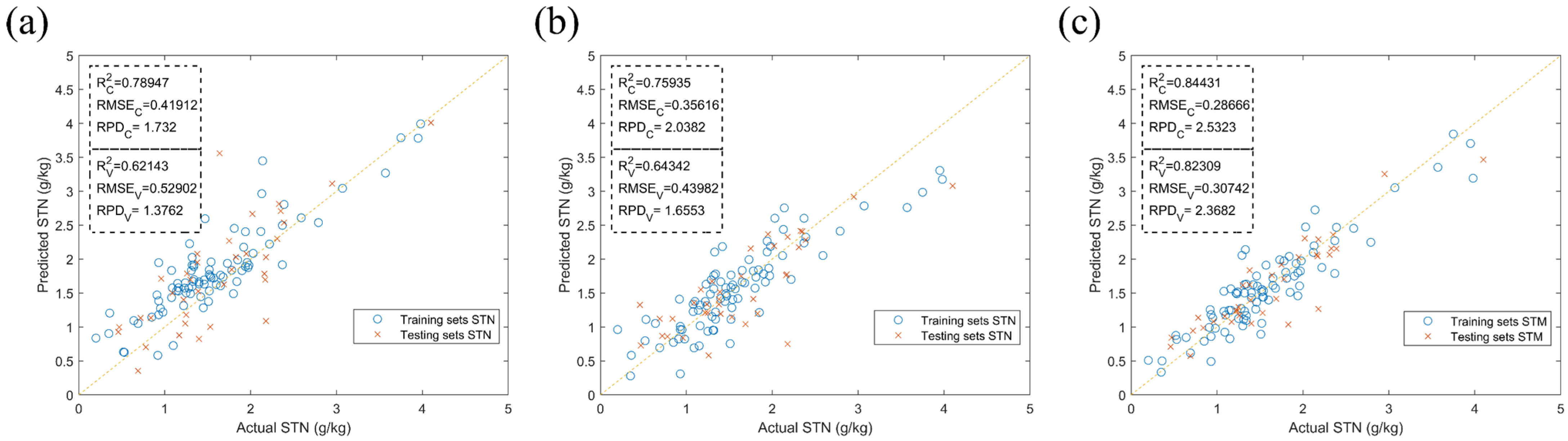
3.1. Preliminary Modeling Results

The initial modeling refers to the development of an evaluation prediction model based on the training set (121 samples × 60 features) of the initial soil total nitrogen feature space (ISTNFS) and the chemically true values of the total nitrogen content of the corresponding soil samples, and the application of a test set to validate the prediction performance of the model. The test set performance metrics of the three prediction models without optimization treatment are obtained to facilitate the next comparison. To optimize the effect for general applicability, this study investigated the relationship between soil olfactory characteristics and soil total nitrogen content through the initial modeling calibration effect of three commonly used prediction models for soil olfactory characteristics, BPNN model, ELM model, and PLSR model.

The BPNN prediction model was constructed based on ISTNFS using H as 8 and predicted in the test set. Figure 5a shows the prediction results of R²_V = 0.62413, RMSE_V = 0.52902, and RPD_V = 1.3762 for the test set. Based on the classification of soil properties RPD, the model RPD_V < 1.5 and the model is not available. The implied layer neurons were set to 20, and the results are shown in Figure 5b, 1.5 < RPD_V < 2.0, the model can only be used to distinguish between high and low values. Six pairs of principal component factors were preferably selected to construct the PLSR prediction model and predicted on the test set, and the prediction results can be obtained from Figure 5c, R²_V = 0.82309, RMSE_V = 0.30742, RPD_V = 2.3682. Since 2.0 < RPD_V < 2.5, the constructed PLSR model can be used for coarse quantitative prediction.

The preliminary modeling results showed that all three assessment models, BPNN, ELM, and PLSR, had some predictive ability of soil total nitrogen content with R²_V greater than 0.5 for the test set. This indicates that there is some correlation between ISTNFS and soil total nitrogen content. However, ISTNFS was not fully optimized, therefore further analysis is needed to determine whether other interferences exist.

3.2. Abnormal Sample Rejection Results

To eliminate the influence of abnormal samples on the later model prediction effect, the soil total nitrogen feature space data included a total of 121 samples. In this study, two different abnormal sample identification methods, MCCV and K-means LOOCV, were used to detect the abnormal samples within the soil total nitrogen feature space.

In the process of identifying abnormal samples in the soil olfactory feature space using the MCCV method, 85 (121 × 70%) samples were first randomly selected from the feature space to construct 1000 BPNN models, and the remaining 36 samples were used for prediction. Figure 6 shows the variation curve of the value of $f_{ac}$ for each sample with the model number after sorting, and the inset of the figure shows the $f_{ac}$ for each sample of the 121 models. It can be seen from the figure that as the number of models increases (i.e., as PRESS increases), the $f_{ac}$ converges to a sampling rate of 70% for each sample in the training set, but the $f_{ac}$ curves for samples 6, 23, 38, 86, 91, and 93 are somewhat different from the other curves in that their $f_{ac}$ values remain greater than 80% in a larger range (model number ≥ 300) as the model serial number increases. Therefore, these six samples were identified as outliers and could be considered abnormal samples.

When K-means LOOCV is used to detect abnormal samples in soil olfactory feature space, it must be clustered first, as shown in

Table 3. K-means clustering results.

Class Number	Number of Samples	Sample Number
Class 1	17	5 16 18 32 39 41 45 63 75 76 80 81 82 84 85 93 118
Class 2	6	20 29 43 73 86 113
Class 3	16	1 13 62 72 74 79 92 102 103 104 111 115 116 119 120 121
Class 4	18	17 19 22 27 28 30 35 40 44 48 58 78 83 89 91 97 109 117
Class 5	13	3 8 9 10 14 25 34 47 56 61 77 96 107
Class 6	4	49 65 68 114
Class 7	2	42 88
Class 8	18	4 6 11 15 23 24 26 38 51 52 69 90 100 101 105 106 108 112
Class 9	14	2 12 21 31 46 50 54 59 60 64 66 70 87 98
Class 10	13	7 33 36 37 53 57 67 71 94 95 99 110

, into 10 classes. According to the principle that abnormal samples are more discrete than normal samples, class 6 and class 7 have the least number of samples, and they are regarded as suspicious abnormal samples and used as prediction samples, and the relative prediction error of suspicious samples is obtained by using the LOOCV method. The results of K-means LOOCV abnormal sample detection are shown in Figure 7. The threshold of abnormal sample determination is set to 0.2 in the figure, and only sample number 88 is found to be an abnormal sample.

According to the empirical Formula (10) and RMSE validation, the number of hidden layer neurons was selected as 8 for the BPNN model. On this basis,

Table 4. Comparison results of different abnormal sample rejection methods.

Types of Rejection Methods	Number of Training Set Samples	Test Set Number of Samples	Number of Neurons in the Hidden Layer	BPNN Model Test Set Prediction Performance
				R2V	RMSEV	RPDV
MCCV	81	34	8	0.75671	0.33517	1.7938
K-means LOOCV	84	36	8	0.69951	0.42919	1.6728

was obtained. The MCCV and K-means LOOCV were used to reject 6 and 1 abnormal samples on the data set, respectively, and all model indexes were improved, among which the MCCV method had the best rejection effect, where R²_V, RMSE_V, and RPD_V were 0.75671, 0.33517, and 1.7938, respectively.

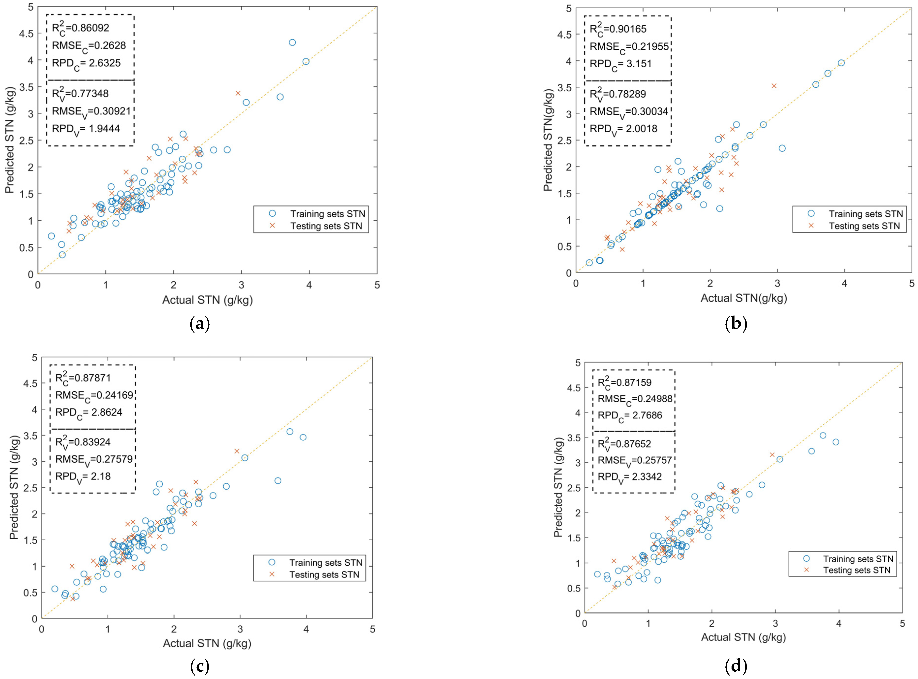
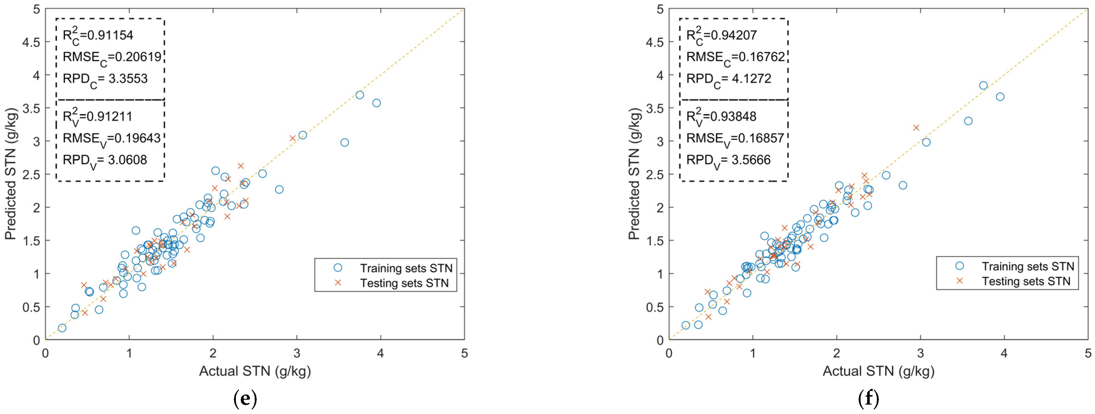
3.3. Feature Optimization Results

To obtain the optimization of feature space by PCA, the new soil olfactory space based on the abnormal samples removed by MCCV (115 samples × 60 features) is referred to as updated soil total nitrogen feature space (USTNFS) and optimized by PCA method with the contribution of variance information of each principal component as pi, and the cumulative contribution of variance information (G(k)) set to 95%, and the results are obtained as in Figure 8. As can be observed from the figure, the cumulative contribution rate of variance information of the first 15 principal components is 94.32%, which can basically reflect the amount of information in the original feature space, i.e., the original feature space can be reduced to 15 dimensions and reconstruct a sample set (115 samples × 15 features).

Similarly, the GA-BP method is used for USTNFS to optimize its features, and the output condition is set to 100 iterations. Figure 9 shows the evolution curve of the fitness function, from which it can be seen that the best fitness curve remains unchanged when the number of species iterations exceeds 32, indicating that it has been optimized to the best effect. At this time, the number of the filtered set of optimal feature vectors are: 1, 2, 4, 6, 7, 10, 12, 16, 18, 20, 21, 23, 24, 25, 27, 29, 30, 32, 33, 34, 36, 40, 41, 43, 45, 46, 47, 51, 52, 53, 55, 58, and the original feature space is reduced from 60 dimensions to 32 dimensions. A sample set (115 samples × 32 features) based on GA-BP optimization was reconstructed.

In the case of comparing the feature selection effects of two feature optimization methods, PCA and GA-BP, the features preferred by the two methods are trained to the corresponding prediction models by BPNN, ELM, and PLSR algorithms, and the test set (34 samples) data are used to verify the models.

In constructing the model using BPNN, due to the reduction of feature dimension, the range of the number of neurons (H) in the hidden layer can be determined according to the formula: 6–15, and the modeling preferred H is 10. As shown in Figure 10a,b, the difference between GA-BP and PCA optimization is small, and GA-BP is slightly better than PCA. When building the ELM model, the GA-BP optimization shown in Figure 10c,d has values 0.1542 and 0.03728 higher than the PCA processed models RPD_V and R², and the RMSE_V is reduced by 0.0182. The preferred modeling principal component factor (PCF) is 4 when modeling and is constructed using PLSR, after cross-validation of RMSE_C and bare pool information criterion Akaike Information Criterion (AIC) evaluation. The modeling parameters are preferred, and the model prediction results are shown in Figure 10e,f. The values of RPD_V and R² of the model are 0.5058 and 0.02637 higher and the RMSE_V is reduced by 0.02786 after GA-BP optimization compared to PCA treatment as shown in Figure 10e,f.

3.4. Discussion

In a bid to verify whether the optimized processing (i.e., MCCV anomaly rejection, GA-BP feature dimensionality reduction) is generalizable for artificial olfaction-based detection of total nitrogen models, three models, BPNN, ELM, and PLSR, were developed and evaluation metrics for each model test set were obtained as in

Table 5. Test set data.

Models	Feature Space of Optimization Process	R2V	RMSEV	RPDV
BPNN	Unoptimized	0.62143	0.52902	1.3762
	MCCV	0.75671	0.33517	1.6553
	MCCV + GA − BP	0.78289	0.30034	2.0018
ELM	Unoptimized	0.64342	0.43982	1.6553
	MCCV	0.82808	0.29323	2.0504
	MCCV + GA − BP	0.87652	0.25757	2.3342
PLSR	Unoptimized	0.82309	0.30742	2.3682
	MCCV	0.89342	0.19556	3.0305
	MCCV + GA − BP	0.93848	0.16857	3.5666

.

The presence of outliers may overestimate or underestimate prediction accuracy, especially when dealing with medium or small datasets [38,39], and after the first stage of optimization processing (MCCV processing), all models R²_V and RMSE_V, and RPD_V were improved. The MCCV method simulates a stochastic process where data with constant replacement are drawn at random each time to form the training set and the remaining data set to form the test set. The model was validated with 1000 repeated random subsamples and is considered an unbiased estimate that is not prone to overfitting [40] as it has been sorted by PRESS values and as the model increases, all those greater than the cumulative probability should be eliminated, as the exclusion of outliers indicates that the MCCV method effectively detects outlier samples. The LOOCV was asymptotically inconsistent, meaning that this method could lead to over-fitting, with good in-sample performance and poor out-of-sample performance, resulting in unreliable estimates. In terms of optimizing the feature dimensionality of the soil olfactory all-nitrogen feature space, after the second stage of optimization processing (GA-BP feature dimensionality reduction), the comparison with the PCA method may be due to the fact that while PCA reduces the olfactory feature dimensionality to 15 dimensions, it discards some of the useful amounts of information, whereas GA-BP uses the GA algorithm with global optimal search capability to seek maximal feature space. Therefore, the optimization process improved the model prediction ability and better reflected the correlation between ISTNFS and total soil nitrogen.

4. Conclusions

The main contribution point of this study is to select the sample rejection method and feature reduction algorithm with better effect and apply it to solve the problem of prediction accuracy of STN based on manual olfaction. The experimental results showed that:

(1)

All two sample rejection methods had gains in the accuracy of soil total nitrogen content prediction. The most significant effect of ISTNFS rejection was MCCV, and the BPNN model indexes improved by 21.76% and 30.34% and reduced by 36.64% in RMSE_V compared to R²_V and RPD_V before the rejection treatment.

(2)

After MCCV to eliminate abnormal samples, GA-BP method has more advantages than PCA method in soil feature space (USTNFS) dimensionality reduction processing under the same model, and can achieve higher prediction performance.

(3)

After optimizing the treatment of ISTNFS using MCCV and GA-BP methods, the prediction performance of the three models, BPNN, ELM, and PLSR, increased by 45.45%, 41.01%, and 50.60% for RPD, 25.98%, 36.33%, and 14.01% for R², and reduced by 76.14%, 70.75%, and 82.36%.

This study can provide a reference for artificial olfaction system data processing of data information in other fields. With the continued refinement of manual sniffing technology, it promises to be an efficient, non-destructive, and inexpensive method of testing for total soil nitrogen content.

References

1. Song, X.; Gao, Y.; Liu, Z.; Zhang, M.; Wan, Y.; Yu, X.; Liu, W.; Li, L. Development of a predictive tool for rapid assessment of soil total nitrogen in wheat-corn double cropping system with hyperspectral data. Environ. Pollut. Bioavailab. 2019, 31, 272–281. [Google Scholar] [CrossRef]
2. Li, M.; Li, R.; Zhang, J.; Wu, T.; Liu, S.; Hei, Z.; Qiu, S. Effects of the integration of mixed-cropping and rice–duck co-culture on rice yield and soil nutrients in southern China. J. Sci. Food Agric. 2020, 100, 277–286. [Google Scholar] [CrossRef] [PubMed]
3. Klem, K.; Záhora, J.; Zemek, F.; Trunda, P.; Tůma, I.; Novotná, K.; Hodaňová, P.; Rapantová, B.; Hanuš, J.; Vavříková, J.; et al. Interactive effects of water deficit and nitrogen nutrition on winter wheat remote rensing methods for their detection. Agric. Water Manag. 2018, 210, 171–184. [Google Scholar] [CrossRef]
4. Lin, L.; Gao, Z.; Liu, X. Estimation of soil total nitrogen using the synthetic color learning machine (SCLM) method and hyperspectral Data. Geoderma 2020, 380, 114664. [Google Scholar] [CrossRef]
5. Li, H.; Yao, Y.; Zhang, X.; Zhu, H.; Wei, X. Changes in soil physical and hydraulic properties following the conversion of forest to cropland in the black soil region of northeast China. Catena 2021, 198, 104986. [Google Scholar] [CrossRef]
6. Zhang, J.; Tian, Y.; Yao, X.; Cao, W.; Ma, X.; Zhu, Y. Estimating model of soil total nitrogen content based on near-infrared spectroscopy analysis. Trans. CSAE 2012, 28, 183–188, (In Chinese with English Abstract). [Google Scholar] [CrossRef]
7. Zhang, D.; Zhao, Y.; Qin, K. A new spectral parametric model for predicting nutrient content of black soils. Spectrosc. Spectr. Anal. 2018, 38, 2932–2936, (In Chinese with English Abstract). [Google Scholar]
8. Li, H.; Jia, S.; Le, Z. Quantitative analysis of soil total nitrogen using hyperspectral imaging technology with extreme learning machine. Sensors 2019, 19, 4355. [Google Scholar] [CrossRef] [Green Version]
9. Pechanec, V.; Mráz, A.; Rozkošný, L.; Vyvlečka, P. Usage of airborne hyperspectral imaging data for identifying spatial variability of soil nitrogen content. ISPRS Int. J. Geo-Inf. 2021, 10, 355. [Google Scholar] [CrossRef]
10. Cheng, Z.; Lu, Z. A novel efficient feature dimensionality reduction method and its application in engineering. Complexity 2018, 2018, 2879640. [Google Scholar] [CrossRef] [Green Version]
11. Shi, B.; Zhao, L.; Liu, W.; Wang, H.; Zhu, D.; Yin, J. Analysis of abnormal samples detected by NIR spectroscopy of apple internal quality. Trans. Chin. Soc. Agric. Mach. 2010, 42, 132–137, (In Chinese with English Abstract). [Google Scholar] [CrossRef]
12. Ma, J.; Yuan, Y. Dimension reduction of image deep feature using PCA. J. Vis. Commun. Image Represent. 2019, 63, 102578. [Google Scholar] [CrossRef]
13. Xu, K.; Wang, J.; Wei, Z.; Deng, F. An optimization of the MOS electronic nose sensor array for the detection of Chinese pecan quality. J. Food Eng. 2017, 203, 25–31. [Google Scholar] [CrossRef]
14. Pham, V.; Weindorf, D.C.; Dang, T. Soil profile analysis using interactive visualizations, machine learning, and deep learning. Comput. Electron. Agric. 2021, 191, 106539. [Google Scholar] [CrossRef]
15. Morellos, A.; Pantazi, X.-E.; Moshou, D.; Alexandridis, T.; Whetton, R.; Tziotzios, G.; Wiebensohn, J.; Bill, R.; Mouazen, A.M. Machine learning based prediction of soil total nitrogen, organic carbon and moisture content by using VIS-NIR spectroscopy. Biosyst. Eng. 2016, 152, 104–116. [Google Scholar] [CrossRef] [Green Version]
16. Olaya, J.F.C.; Ordoñez, M.C.; Salcedo, J.R. Impact of nutritional management on available mineral nitrogen and soil quality properties in coffee agroecosystems. Agriculture 2019, 9, 260. [Google Scholar] [CrossRef] [Green Version]
17. Gu, S.; Wang, J.; Wang, Y. Early discrimination and growth tracking of aspergillus spp. contamination in rice kernels using electronic nose. Food Chem. 2019, 292, 325–335. [Google Scholar] [CrossRef]
18. Wang, X.; Zhou, W.; Liang, G.; Song, D.; Zhang, X. Characteristics of maize biochar with different pyrolysis temperatures and its effects on organic carbon, nitrogen and enzymatic activities after addition to fluvo-aquic soil. Sci. Total Environ. 2015, 538, 137–144. [Google Scholar] [CrossRef]
19. Liu, R.; Chen, W.; Xu, K.; Qiu, Q.; Cui, H. Application of rapid singularity detection in Near-Infrared Spectroscopy for milk composition measurement. Spectrosc. Spectr. Anal. 2005, 25, 207–210, (In Chinese with English Abstract). [Google Scholar] [CrossRef]
20. Shapiro, A. Monte Carlo sampling methods. Handb. Oper. Res. Manag. Sci. 2003, 10, 353–425. [Google Scholar] [CrossRef]
21. Li, X.; Wei, Y.; Xu, J.; Xu, N.; He, Y. Quantitative visualization of lignocellulose components in transverse sections of moso bamboo based on ftir macro- and micro-spectroscopy coupled with chemometrics. Biotechnol. Biofuels 2018, 11, 263. [Google Scholar] [CrossRef] [Green Version]
22. Liu, C.; Hu, Y.; Wu, S.; Sun, X.; Dou, S.; Miao, Y.; Dou, Y. A study of Near-Infrared Spectral singular sample rejection method. J. Food Sci. Technol. 2014, 32, 74–79, (In Chinese with English Abstract). [Google Scholar] [CrossRef]
23. Li, J.; Sun, L.; Li, Y.; Lu, Y.; Pan, X.; Zhang, X.; Liu, Y.; Song, Z. Rapid prediction of acid detergent fiber content in corn stover based on NIR-Spectroscopy technology. Optik 2019, 180, 34–45. [Google Scholar] [CrossRef]
24. Jirayucharoensak, S.; Pan-Ngum, S.; Israsena, P. EEG-Based emotion recognition using deep learning network with principal component based covariate shift adaptation. Sci. World J. 2014, 2014, 627892. [Google Scholar] [CrossRef] [Green Version]
25. Assi, K. Traffic crash severity prediction—A synergy by hybrid principal component analysis and machine learning models. Int. J. Environ. Res. Public Health 2020, 17, 7598. [Google Scholar] [CrossRef]
26. He, H.; Tian, C.; Jin, G.; Han, K. Principal component analysis and fisher discriminant analysis of environmental and ecological quality, and the impacts of coal mining in an environmentally sensitive area. Environ. Monit. Assess. 2020, 192, 207. [Google Scholar] [CrossRef]
27. Wang, J. Analysis of sports performance prediction model based on GA-BP neural network algorithm. Comput. Intell. Neurosci. 2021, 2021, 4091821. [Google Scholar] [CrossRef]
28. Wang, L.; Bi, X. Risk assessment of knowledge fusion in an innovation ecosystem based on a GA-BP neural network. Cogn. Syst. Res. 2020, 66, 201–210. [Google Scholar] [CrossRef]
29. Jiang, G.; Grafton, M.; Pearson, D.; Bretherton, M.; Holmes, A. Integration of precision farming data and spatial statistical modelling to interpret field-scale maize productivity. Agriculture 2019, 9, 237. [Google Scholar] [CrossRef] [Green Version]
30. Zhao, J.; Yang, D.; Wu, J.; Meng, X.; Li, X.; Wu, G.; Miao, Z.; Chu, R.; Yu, S. Prediction of temperature and CO concentration fields based on BPNN in low-temperature coal oxidation. Thermochim. Acta 2021, 695, 178820. [Google Scholar] [CrossRef]
31. Zhang, W.; Zhou, J.; Yu, B.; Yu, Y. Construction of BPNN-based optimization model for spherical bow resistance reduction. J. Dalian Univ. Technol. 2021, 61, 160–171, (In Chinese with English Abstract). [Google Scholar] [CrossRef]
32. Yin, S.; Liu, H.; Duan, Z. Hourly PM2.5 Concentration multi-step forecasting method based on extreme learning machine, boosting algorithm and error correction model. Digit. Signal Process. 2021, 118, 103221. [Google Scholar] [CrossRef]
33. Zhang, X.; Huang, B. Prediction of soil salinity with soil-reflected spectra: A comparison of two regression methods. Sci. Rep. 2019, 9, 5067. [Google Scholar] [CrossRef]
34. Wang, Y.; Li, M.; Li, L.; Ning, J.; Zhang, Z. Green analytical assay for the quality assessment of tea by using pocket-sized NIR spectrometer. Food Chem. 2021, 345, 128816. [Google Scholar] [CrossRef]
35. Zhu, L.; Jia, H.; Chen, Y.; Wang, Q.; Li, M.; Huang, D.; Bai, Y. A novel method for soil organic matter determination by using an artificial olfactory system. Sensors 2019, 19, 3417. [Google Scholar] [CrossRef] [Green Version]
36. Dai, Y.; Zhou, B.; Wang, J. Application of electronic nose in detection of cotton bollworm infestation at an early stage. Trans. CSAE 2020, 36, 313–320, (In Chinese with English Abstract). [Google Scholar] [CrossRef]
37. Michael, V.; Joachim, B.; Joachim, H.; Heinz-Christian, F. Comparing different multivariate calibration methods for the determination of soil organic carbon pools with visible to near infrared spectroscopy. Geoderma 2011, 1, 198–205. [Google Scholar] [CrossRef]
38. Zulj, S.; Carvalho, P.; Ribeiro, R.T.; Andrade, R.; Magjarevic, R. Data size considerations and hyperparameter choices in case-based rea-soning approach to glucose prediction. Biocybern. Biomed. Eng. 2021, 41, 733–745. [Google Scholar] [CrossRef]
39. Nakatsu, R.T. An Evaluation of Four Resampling Methods Used in Machine Learning Classification. IEEE Intell. Syst. 2020, 36, 51–57. [Google Scholar] [CrossRef]
40. Barrow, D.K.; Crone, S.F. Cross-validation aggregation for combining autoregressive neural network forecasts. Int. J. Forecast. 2016, 32, 1120–1137. [Google Scholar] [CrossRef] [Green Version]
Figure 1. Study area and sampling locations.
Agriculture 12 00037 g001
Figure 2. Thermal cracking-based artificial olfactory system for soil total nitrogen detection system. 1. Gas sensor array 2. Vacuum flange 3. Vacuum pump 4. PWN module 5. 12V power supply 6. Gas chamber 7. Signal processing circuit 8. NI data acquisition card 9. Muffle furnace 10. Computer.
Agriculture 12 00037 g002
Figure 3. Sensor response curves: (a) 0.2 g·kg−1 soil sample; (b) 4.1 g·kg−1 soil sample.
Agriculture 12 00037 g003
Figure 4. GA-BP flow chart.
Agriculture 12 00037 g004
Figure 5. Graph of prediction results of three models for initial modeling. (a) Initial modeling BPNN model prediction results. (b) Initial modeling ELM model prediction result. (c) Initial modeling PLSR model prediction result.
Agriculture 12 00037 g005
Figure 6. Cumulative frequency profile of each sample.
Agriculture 12 00037 g006
Figure 7. K-means LOOCV detection of abnormal sample results.
Agriculture 12 00037 g007
Figure 8. Cumulative contribution results of PCA principal components.
Agriculture 12 00037 g008
Figure 9. Evolutionary plot of optimal fitness function.
Agriculture 12 00037 g009
Figure 10. Results of three models after optimization of PCA and GA-BP features. (a) Prediction results of BPNN model after PCA optimization. (b) GA-BP optimized BPNN model prediction results. (c) Prediction results of ELM model after PCA optimization. (d) Prediction results of ELM model after GA-BP optimization. (e) Prediction results of PLSR model after PCA optimization. (f) Prediction results of PLSR model after GA-BP optimization.
Agriculture 12 00037 g010aAgriculture 12 00037 g010b