Article

Yield Components Stability Assessment of Peas in Conventional and Low-Input Cultivation Systems

by
Vasileios Greveniotis
1,2,*,
Elisavet Bouloumpasi
3,
Stylianos Zotis
2,†,
Athanasios Korkovelos
4 and
Constantinos G. Ipsilandis
5
1
Hellenic Agricultural Organization Demeter, Institute of Industrial and Forage Crops, GR-41335 Larissa, Greece
2
Department of Agricultural Technology, Technological Educational Institute of Western Macedonia, GR-53100 Florina, Greece
3
Department of Agricultural Biotechnology and Oenology, International Hellenic University, GR-66100 Drama, Greece
4
Directorate of Water Management of Thessaly, Decentralized Administration of Thessaly—Central Greece, GR-41335 Larissa, Greece
5
Regional Administration of Central Macedonia, Department of Agriculture, GR-54622 Thessaloniki, Greece
*
Author to whom correspondence should be addressed.
Deceased.
Agriculture 2021, 11(9), 805; https://doi.org/10.3390/agriculture11090805
Submission received: 19 July 2021 / Revised: 21 August 2021 / Accepted: 23 August 2021 / Published: 24 August 2021
(This article belongs to the Special Issue Crop Breeding and Genetics)

Abstract

:
The primary purpose of this study was to explore yield stability of pea (Pisum sativum L.) cultivars based on stability index, with specific aim at studying cultivar behavior regarding yield of peas under both conventional and low-input cultivation systems. Five cultivars of peas were used in a strip-plot design. Correlations showed a significant positive relation between seed yield and some other traits. Indirect seed yield improvement may be implemented by improving pod length, which generally showed high stability indices in Greek mega-environment. Comparisons between conventional and low-input farming systems generally did not affect stability estimations, but revealed cultivars that exhibited stable performance, even in low-input farming systems. The additive main effects and multiplicative interaction (AMMI) biplot analysis, genotype by environment interaction (GGE) biplot analysis and analysis of variance (ANOVA) showed statistically significant differences between genotypes and environments, and also the farming system. This way, we have certain cultivars of peas to recommend for specific areas and farming system, in order to achieve the most stable performance. Vermio proved to be a stable cultivar for seed yield performance, in Giannitsa, Trikala and Kalambaka area, in low-inputs farming systems, while Olympos was the best in Florina area and low-input farming.

1. Introduction

Pea (Pisum sativum L.), is an herbaceous winter annual and self-pollinated crop. In terms of nutritive value peas contain a high percentage (ranging from 15% to 35%) of proteins including the essential amino acids tryptophan and lysine, and also a significant content of vitamins, minerals and carbohydrates [1,2]. Peas can grow in a wide range of agro-climatic zones, which provides a tremendous scope and potential for cultivation of this crop. According to the Food and Agriculture Organization (FAO) data, peas covered an area of 7,166,876 ha in 2019. Worldwide production of dry peas in 2019 exceeded 14 million tonnes, while over 5 million tonnes were produced in Europe [3]. Pulses as a group of crop species are mainly cultivated in South Asia and Sub-Saharan Africa with the crop exhibiting an increasing yield trend [4]. However, low productivity of the crop has created the necessity to breed new high yielding cultivars, which may fulfil the needs of the growers and enhance the productivity. Various planning and execution of a breeding program for the improvement of the various quantitative traits depend, to a great extent, upon the magnitude of genetic variability existing in the population. The genetic variability forms the basis of the entire breeding program. Selection cannot be effective in population without variability. To give a better insight of ancillary characters under selection, genetic variability analysis is the tool, which is being effectively used for determining the rate of various yield components in different crops, leading to the selection superior genotypes [5,6]. Therefore, for a rational approach to the improvement of vegetable yield, it is imperative to have information on the association among different yield and its component. Existence of sufficient variability in the genetic stock is a prerequisite for initiation of any breeding program. On the basis of above points the present study was conducted to estimate the genetic parameters for growth and yield parameters in pea.
Fasoulas [7] based on other researchers (Edmeades and Daynard [8] and Tollenaar and Wu [9]) proposed the ratio 1/CV (reversed coefficient of variation) between mean and standard deviation for estimating stability and, as an improvement, Fasoula [10] used the squared form as a stability criterion (stability index).
In peas, many researchers assessed stability using different approaches and methods, especially for yield [11,12,13,14], some of them in multi-location environments. All these researchers tried to define the best genotypes suitable for various environments. A cultivar must be considered more adaptive or stable if it has a high mean of yield with low degree of fluctuation in different locations or seasons [7,15]. In our approach this is interpreted in high adaptability when the stability criterion we used, shows high values. Acikgoz et al. [11] showed that cluster analysis was more efficient than classic stability analysis. The most recent research involves Genotype x Environment (GxE) interaction analysis, and that concept was part of our study too, involving ANOVA, GGE (genotype main effect (G) plus genotype by environment interaction (GE)) AMMI biplot analysis and correlations, using additional data to support primary field research in order to improve efficiency of estimations [16,17]. Predictive accuracy of such research trials is described in previous work based on AMMI analyses [18].
The primary purpose of this study was to determine yield stability of pea cultivars and yield correlated traits based on the innovative approach of estimating stability index, with specific aim to study cultivar behavior regarding yield of peas under both conventional and low-input cultivation systems. ANOVA, AMMI and GGE biplot tools are considered proper for multi-environment analyses [17]. Heritability is usually calculated as the ratio of genetic variability to total variability, but Greveniotis et al. [19] used stability index, based on Fasoulas [7] and Fasoula [10] remarks, as an estimation criterion of heritability of various traits, being able to distinguish between qualitative and quantitative traits. In that manner, the approach selected to analyze present data includes stability behavior and the kind of heritability of traits.

2. Materials and Methods

2.1. Crop Establishment and Experimental Procedures

Field experiments were conducted during two growing seasons (2008–2009 and 2009–2010) in four different locations. Two locations in Northern Greece and two locations in Central Greece were selected, varying in soil type and altitude. Coordinates according to the WGS 1984 geographic coordinate system are provided.
(A)
In Giannitsa, Northern Greece (latitude, 40°77′ N; longitude, 22°39′ E; elevation, 10 m a.s.l.). The soil type was clay (C): sand, 9.1%; silt, 37.5%; clay, 53.8%.
(B)
In the farm of the Technological Educational Institute of Western Macedonia in Florina, Northern Greece (latitude, 40°46′ N; longitude, 21°22′ E; elevation, 705 m a.s.l.). The soil type was characterized as a sandy loam (SL): sand, 62%; silt, 26.9%; clay, 11.1%.
(C)
In Trikala, Central, Greece (latitude, 39°55′ N; longitude, 21°64′ E; elevation, 120 m a.s.l.). The soil type was characterized as sandy clay loam (SCL): sand, 48.6%; silt, 19.2%; clay, 32.2%.
(D)
In Kalambaka, Central Greece (latitude, 39°64′ N; longitude, 21°65′ E; elevation, 190 m a.s.l.). The soil type was silty clay (SiC): sand, 14.6%; silt, 41.2%; clay, 44.2%.
Those locations were selected deliberately because of their varied environmental conditions. Basic weather data (mean monthly temperatures in °C and rainfall in mm) for each experimental site based on daily records, for the two growing seasons of the experimentation, are given in Figure 1.
In Figure 2, basic weather data regarding years 2018–2019 and 2019–2020 growing seasons are presented for comparison reasons for all environments, in order to evaluate the experimental areas across time. growing seasons. The agro-climatic conditions across all the four locations in Greece does not have changed significantly and the results are still relevant to the present-day conditions.
Five cultivars of peas, namely, cv. Olympos, cv. Pisso, cv. Livioletta, cv. Vermio and cv. Dodoni, were used. The characteristics of the selected cultivars are given next:
Dodoni is a mid-early to late flowering variety, suitable for hay and seed production, with good adaptability to the wet and cold regions of the country (mainly mountainous and semi-mountainous areas), with cool summers. It is resistant to cold as it withstands winter frosts (temperatures that can reach −18 °C).
Olympos is a relatively late flowering variety. It has good resistance to cold but less than Dodoni. It is generally adaptable to areas with milder winter temperatures. It is suitable mainly for seed production.
Vermio is a relatively late flowering variety. It is suitable for hay production. It is resistant to cold and presents high adaptability to soils with poor to medium fertility.
Pisso is suitable for hay and seed production, also used for silage or grazing. It withstands frost; therefore, it is favored in Northern Greece.
Livioletta is suitable for green manure, grazing, cutting and excellent for summer intercropping. It is resistant to frost and combines high production, very good adaptability and good quality. It produces a high protein content and high dry matter yields.
The cultivation was conducted using a strip-plot design with the five cultivars randomized within each plot. Each plot consisted of seven rows 5 m in length and the rows were spaced 25 cm apart. The plot size was 8.75 m2. Four replications of each plot were used, properly and randomly allocated in the strip-plot design used.
Two types of cultivation approaches were selected: (1) under low-input and (2) under conventional farming systems.
The plots cultivated under the conventional farming system were fertilized before sowing so that 40 and 80 kg ha−1, nitrogen and P2O5, respectively, were added into the soil.
For low-input cultivation, no fertilizers or other agrochemicals were applied during the experiment in all four different locations, while prior to the establishment of the experiment in 2008, the fields had been in a two-year rotation consisting of bread wheat/legume without nutritional supplementation or other agrochemical inputs.
Weeds were controlled by hand in the experimental area. The selected cultivars were sown in early November during November 2008 and November 2009 for growing seasons 2008–2009 and 2009–2010, respectively, and were harvested during physiological maturity stage R8 in late June 2009 and late June 2010 for growing seasons 2008–2009 and 2009–2010, respectively.

2.2. Measurements

The traits measured were as follows:
Seed yield (kg ha−1): corresponds to the weight of seeds obtained from each plot after threshing and cleaning and subsequent calculation on a hectare basis.
Thousand-seed weight per plant (g): corresponds to the seeds of five randomly selected plants from each plot, which were mixed in order to draw a representative sample of 1000-seeds (TSW), and subsequent weigh in grams.
Number of pods per plant: corresponds to the total number of pods per plant counted at the time of maturity and averaged. For this estimation ten plants were randomly selected per plot.
Number of seeds per pod: From each plot ten plants were randomly selected, and five pods were taken from total pods randomly. Total number of seeds of these pods was counted and their mean value was calculated.
Pod length (cm): ten plants were randomly selected per plot and five pods were taken, their length was measured and their mean value was calculated.
Pod width (mm): ten plants were randomly selected per plot. and five pods were taken, their width was measured and their mean value was calculated.
Number of branches per plant: corresponds to the numbers of primary branches per plant, which were counted from ten randomly selected plants, at the stage of complete vegetative growth.
Plant height (cm): ten plants were randomly selected per plot and plant height was measured on sampled plants in centimeters from the ground level to the top of the plant at maturity and average value was calculated.

2.3. Data Analysis

Data primarily analyzed via ANOVA over environments and cultivation practice to experience if there are significant differences for all traits investigated in this study. For the ANOVA table to be more informative the combination of each year and location was assigned as the environment. In this way, we have fewer interactions in the ANOVA table and do not affect the variance of genotypes (cultivars) and the G × E (genotype × environment) interaction which is crucial for proceeding in the stability analysis.
Stability estimations were based on stability index ( x ¯ / s ) 2 , where x ¯ and s are the entry mean yield and the standard deviation, respectively [10,20].
Trait correlations were examined using the Pearson coefficient according to Steel et al. [21], and the significance of all the statistics was checked at p < 0.05 using SPSS ver. 25. Stability analysis was performed using the free version of PB Tools v.1.4. (International Rice Research Institute, Laguna, Philippines) over locations and years for each characteristic and the statistical tools were the AMMI and (GGE) biplot analysis. A Finlay–Wilkinson [22] regression would be useful only for row data on the measurements of each trait. Instead, in our approach, stability index values represent initial stability estimations that were analyzed further by AMMI and GGE biplot analysis for better assessing adaptability and stability. Finlay–Wilkinson charts would be useful only for environment evaluation based on stability index values (Figure 3, based on seed yield stability indices).

3. Results

3.1. ANOVA and Descriptive Statistics on Stability Index

Comparisons between Figure 1 and Figure 2, showed some differences in rainfall that could affect cultivar behavior in present years, where rainfall is reduced. Regarding the ANOVA table (Table 1), the main effects for all traits expressed significant differences. Furthermore, the G × E interaction, showing significant differences for all traits. Multiple interaction involving genotypes, environment and cultivation system was very significant and these data must be analyzed in combination with cultivar performance within each environment and cultivation system. To clarify the performance of the cultivars along environments and estimate the stability of each cultivar for all traits, Fasoula [4,10] method along with AMMI and GGE analysis were performed. Prior to the AMMI analysis it was assessed its appropriateness. For all traits the sum of squares for the GEs signal was more than four times as large as that for G, so the AMMI analysis was likely to be worthwhile (data not shown) [16].
Stability estimations based on the calculation of stability index of each trait are presented in Table 2, Table 3 and Table 4 and represent initial stability estimations.
In Table 2 are tabulated stability index data across environments for the eight characteristics under study. Pod length showed the highest indices across all environments (especially for low inputs Florina, where it reached index value 505). Number of seeds per pod and plant height showed generally high indices. As it was expected, seed yield showed low indices. Low-inputs farming systems seems to improve stability indices in many cases for seed yield, as it was found for Florina.
In Table 3, it is shown the behavior of genotypes in all farming systems. Cultivar Vermio followed by cv. Olympos showed stability performance for seed yield (only for few traits), especially in low-inputs systems.
Table 4 combines data for genotypes across environments and farming systems. This table is useful to depict the most stable cultivar (genotype) for a certain area (environment) and the selected farming system. In Florina area and for the trait seed yield, cv. Vermio exhibited an extremely stable performance with an index up to 596 for low-inputs, while cv. Olympos reached 294. Cultivar Livioletta showed a stability index close to 3.000 for plant height, in Trikala area. Pod length also exhibited high stability indices, although lower than plant height. These data tabulated in Table 4 are the most useful to discuss, because of the multiple significant interaction between factors present.
As it is clearly seen in Figure 3, three environments are considered moderate stable for stability evaluations, since values are concentrated and not spread. Slope-values are generally low, while for one environment slope is near one and cases are spread (Florina). In that case, there are indications that specific cultivars may exhibit extreme stability index values for seed yield.

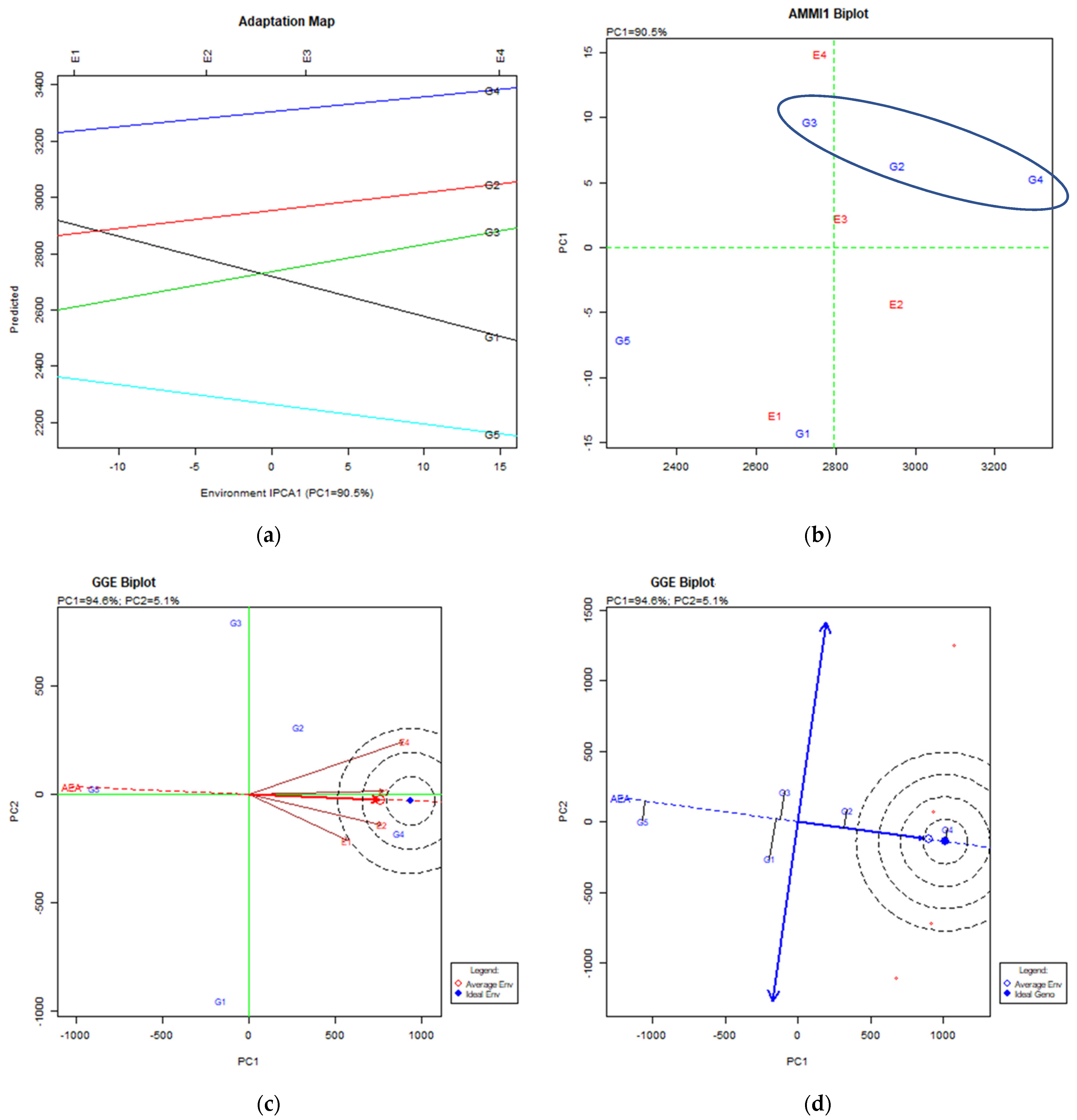
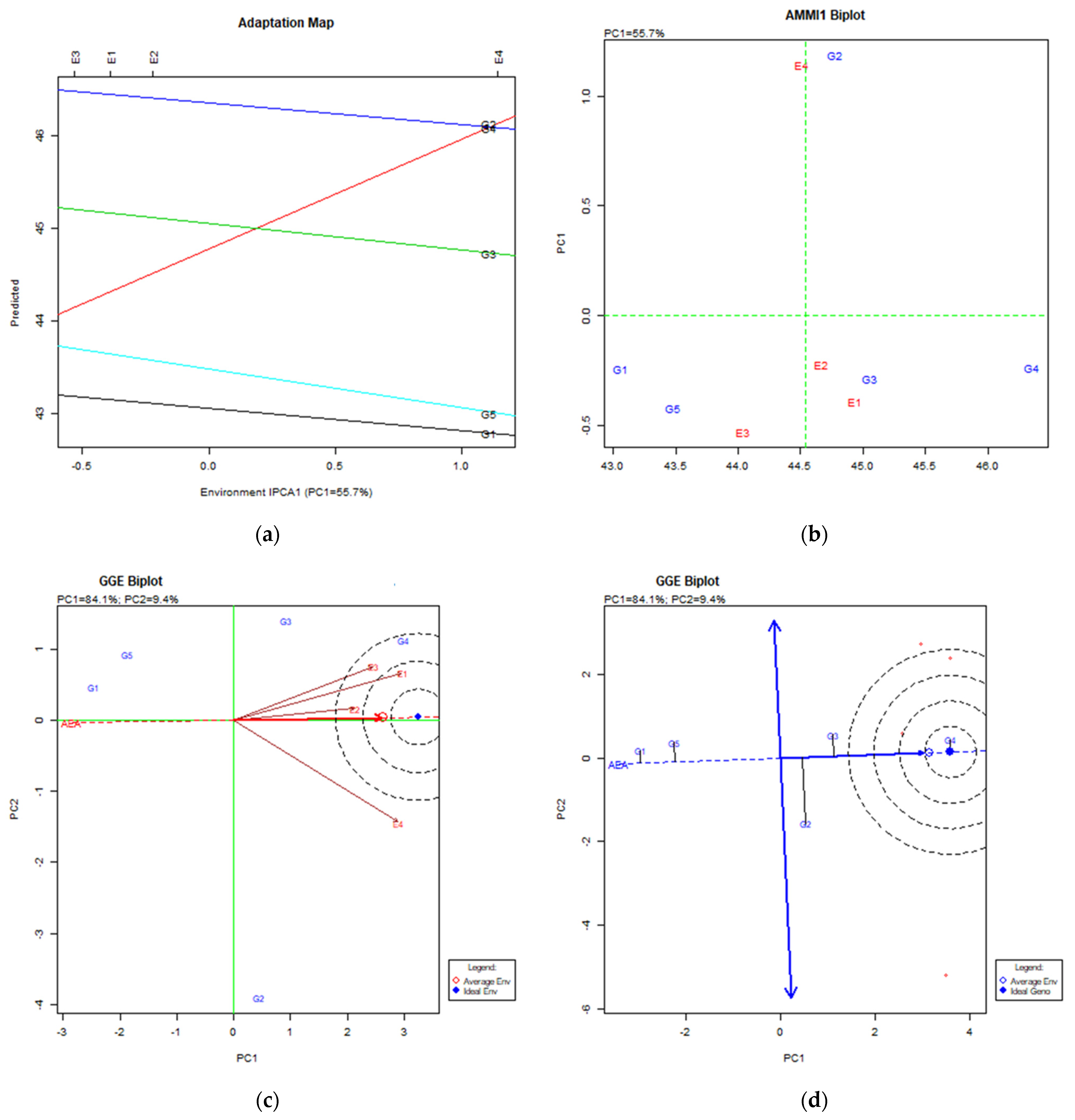
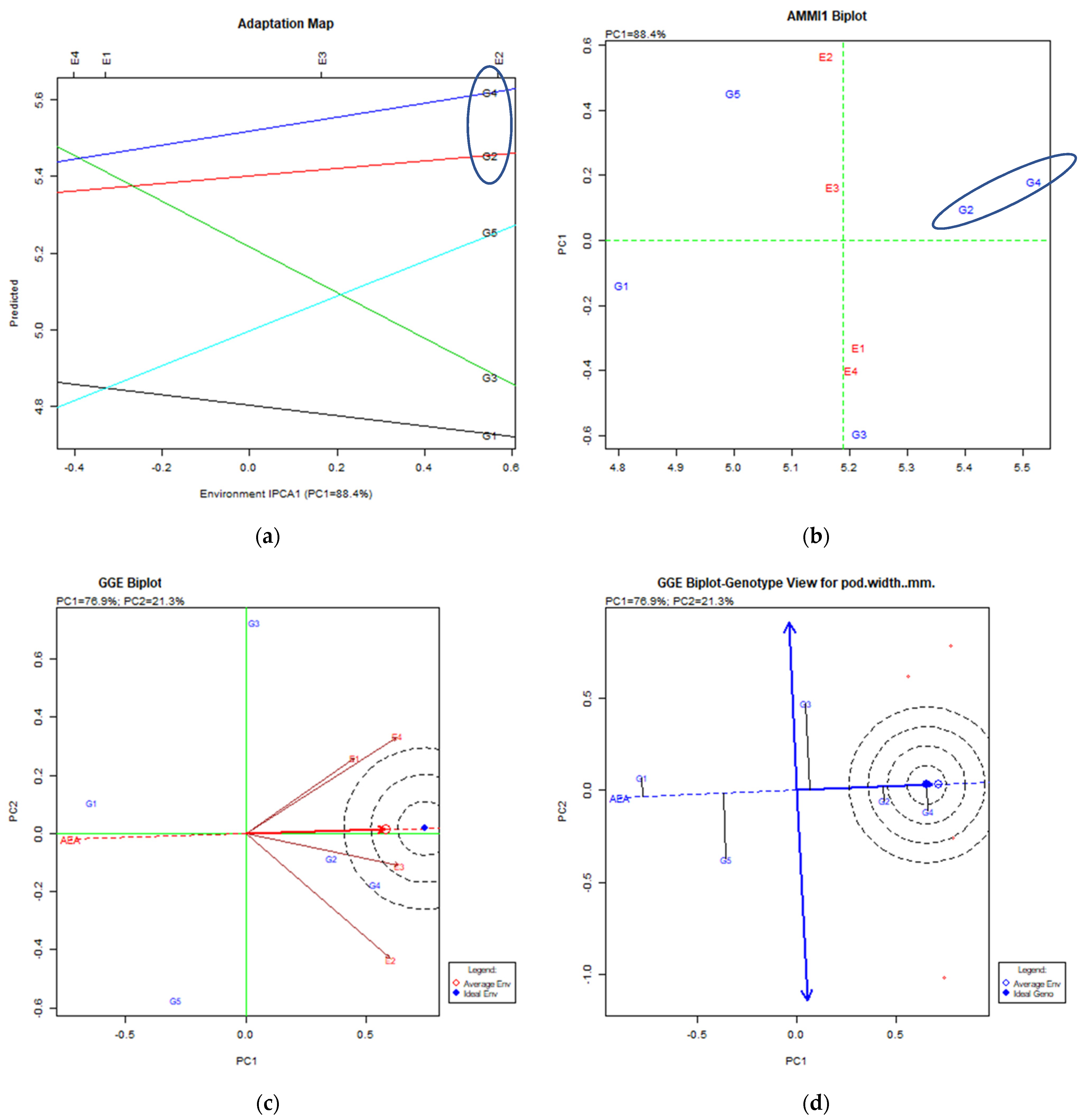
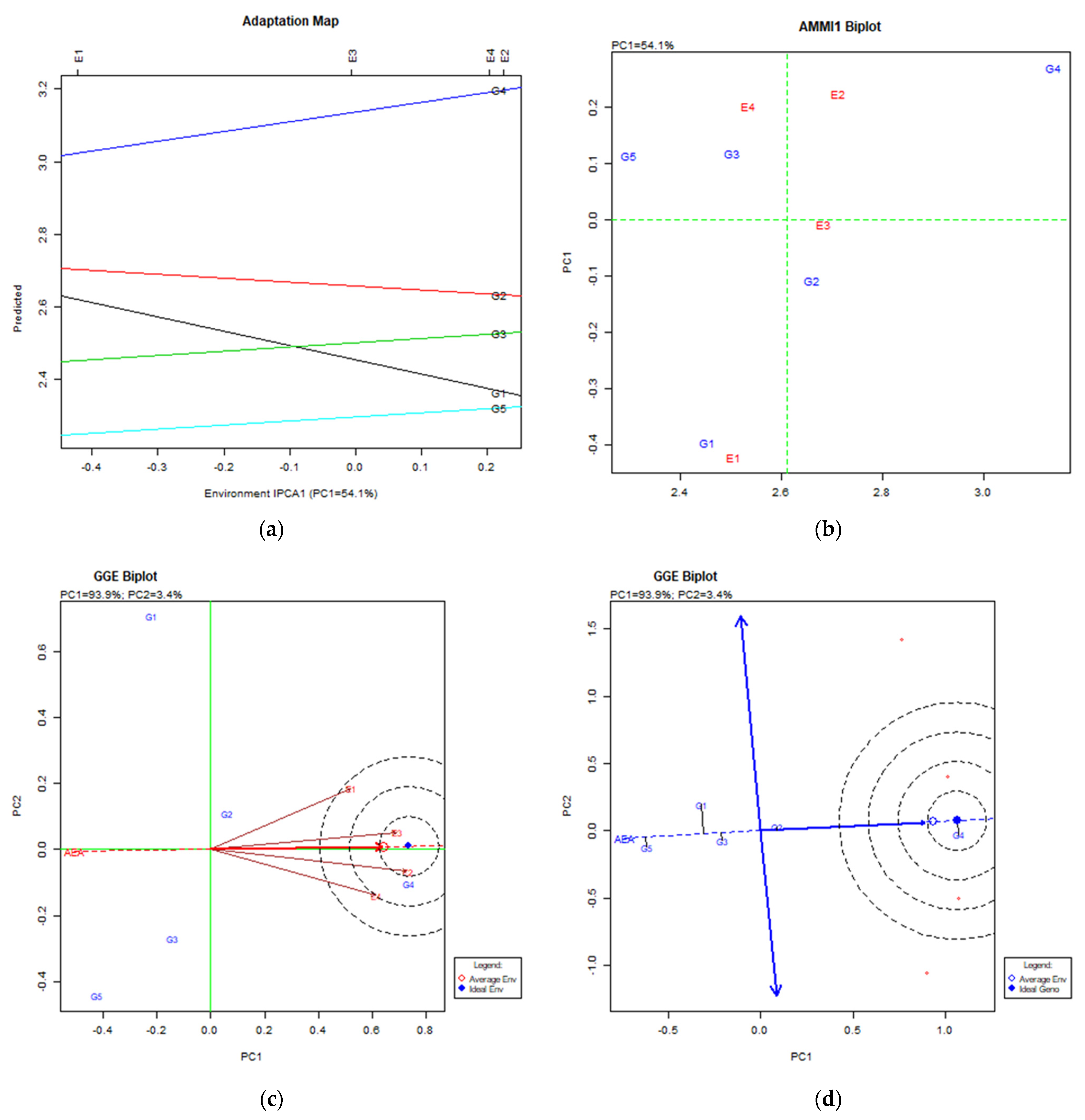
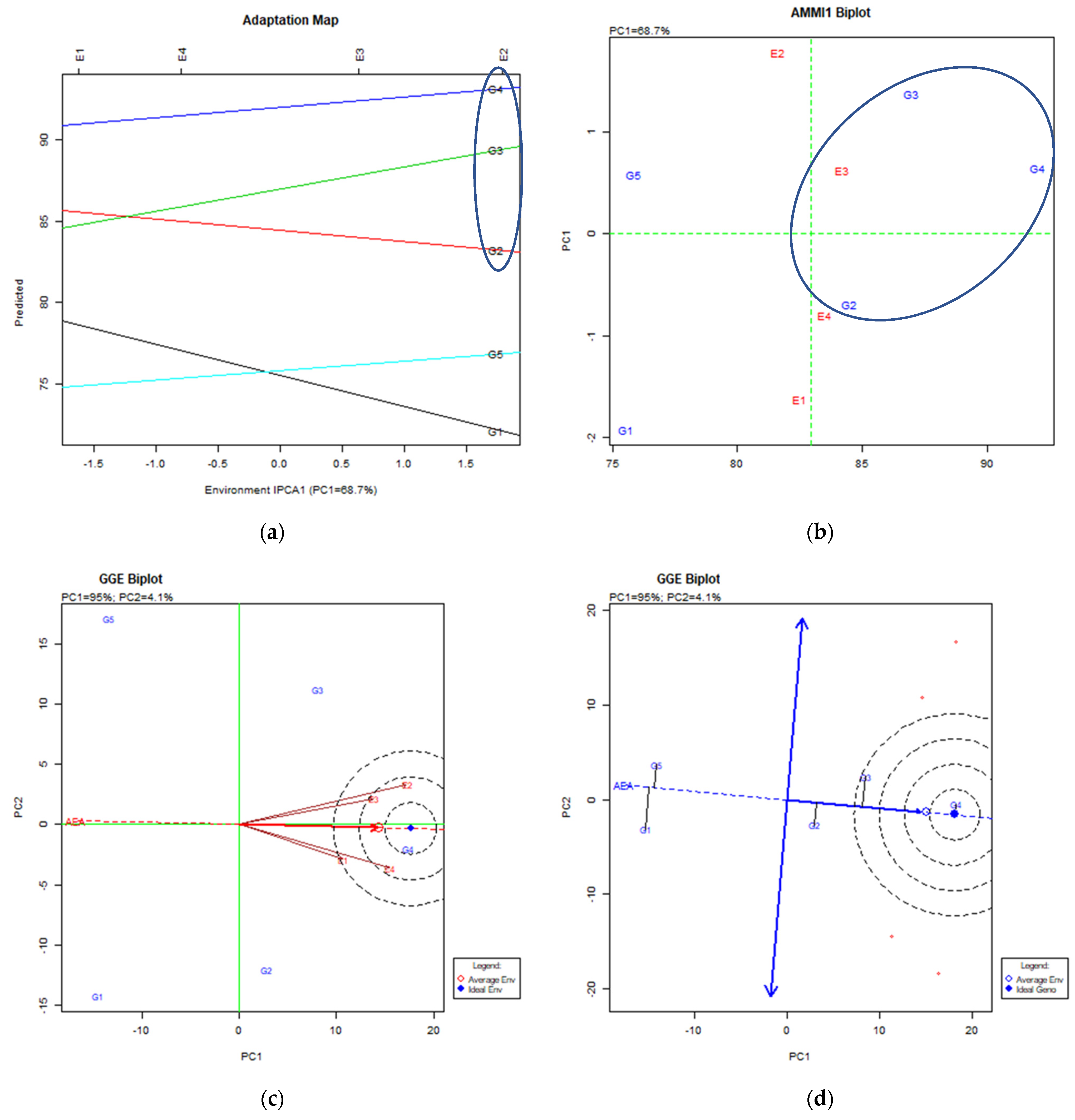
3.2. The AMMI Tool for Multi-Environment Evaluations

The AMMI model is a widely used statistical tool in the analysis of multi-environment experiments. The purpose is to understand the complex GEI. In the AMMI model the data are represented by a two-way table of GEI means. In the complete tables, least squares estimation is equivalent to fitting an additive two-way ANOVA model for the main effects and applying a singular value decomposition to the interaction residuals [23].
Using this statistical tool AMMI software generates mainly the adaptation map and AMMI1 biplot where one axis is the axis of the factor and the other is the PC1 value. When the PC1 value and its distance from the X-axis are close then the factor analyzed is stable. Regarding the AMMI1 biplot, the desirable cultivars were those having high value on the axis of trait performance (X-axis, right position) and close to the center of the PC1 axis (near zero).
GGE stands for genotype main effect (G) plus genotype by environment interaction (GE), which is the only source of variation that is relevant to cultivar evaluation. Mathematically, GGE is the genotype by environment data matrix after the environment means are subtracted.
A GGE biplot is a biplot that displays the GGE of a genotype by environment two-way data. The GGE biplot methodology originates from the graphical analysis of multi-environment cultivar trials (MET) data but is equally applicable to all other types of two-way data. Regarding the GGE biplot for environments, the most stable environment is considered the one placed close to the dot of ideal and average environment and in the concentric area of the ideal environment dot. As far as the GGE biplot for cultivars, the desirable cultivars (stable and productive) were those which placed near to the ideal cultivar and in the concentric area of the ideal cultivar dot.
The AMMI1 and GxE biplot analysis created biplots depicting the performance of the cultivars among environments. The biplots created can easily characterize each cultivar for performance and stability as an easy tool used for that purpose.
Regarding the trait of “seed yield”, the figures produced by the AMMI analysis, adaptation map (Figure 4a) and AMMI1 biplot (Figure 4b) showed that the most productive and stable cultivar over all environments was the G4 followed by the G2 and the G3. Based on the GGE biplot for environments, all cultivars were placed in the concentric area of the ideal environment and very near to the average environment (Figure 4c). Based on the GGE biplot for cultivar the most productive and stabile one was the G4, which placed on the dot of the ideal genotype.
Data from the “thousand seed weight” (TSW) used in AMMI and GGE biplot analysis divided the cultivars in two groups of high and low performance. The high-performance group consisted from the G4 and G2 cultivars, whereas the low performance group consisted from the G1, G3 and G5 cultivars. Both analyses used AMMI and GGE biplot showed that the G4 had the highest thousand seed weight value with relative lower stability, followed from G2 which was very stable across all environments (Figure 5a–d).
The trait “number of pods per plant” for both AMMI and GGE biplot showed that the most productive cultivars were the G4 followed by the G2 (Figure 6a–d). The trait of seed per pod shown that, the most productive cultivar was the G4, followed by G2, both for AMMI and GGE biplot analysis (Figure 7a–d). The stability analysis using AMMI and GGE biplot for pod length (Figure 8a–d) shown that the most productive and stable cultivar was the G4, followed by the G3 characterized of less stability.
The “pod width” trait for both AMMI and GGE biplot, showed that the most stable cultivar was the G4 followed by the G2. The G5 and G2 cultivars shown specific adaptability over the environments (Figure 9a–d). The stability analysis using AMMI and GGE biplot performed on the cultivars for the of trait number of branches per plant shown that the G4 cultivar was the most productive and stable one (Figure 10a–d).
AMMI and GGE biplot analysis for “plant height” trait showed that the most desirable cultivars with relative stability were the G4, followed by the G3 and the G2 (Figure 11a–d).
From AMMI analysis as visualized by the adaptation map (figure (a) in each of the trait figures, Figure 4, Figure 5, Figure 6, Figure 7, Figure 8, Figure 9, Figure 10 and Figure 11), it is clearly seen that the most desirable cultivars were those placed high on the axis of trait performance showing a nearly parallel line to the PC1 axis, which was an indication of stability over the environments. For the AMMI1 biplot, the desirable cultivars were those placed high on the axis of trait performance (X-axis, right position) and close to the center of the PC1 axis (near zero).
Regarding the GGE biplot for environments, the most stable environment was the one placed close to the dot of ideal and average environment and in the concentric area of the ideal environment dot. Concerning GGE biplot for cultivars, the desirable cultivars (stable and productive) were those placed to the ideal cultivar and in the concentric area of the ideal cultivar dot.

3.3. Correlations between Characteristics

In Table 5, correlations between all traits are tabulated. All correlations were highly statistically significance, especially for seed yield to other traits such as the dimensions of pod.

4. Discussion

Both peas’ farmers and breeders are depending on stable performance of various pea characteristics, especially yield.
In our work the two cultivation systems (conventional and low-input) displayed differences in cultivar yielding performance, but overall estimations on various pea characteristics seemed not to be affected. In combination to GGE biplot analysis, the two farming systems revealed the most stable cultivars across all environments, as well as the more stable in specific environments. Additionally, some cultivars exhibited stability in the low-inputs conditions. Generally, there were very significant GGE interactions. Acigioz et al. [11] reported also significant GGE interactions, analyzing dry matter and seed yield in peas.

4.1. Seed Yield

For the trait of seed yield stability analysis results depicted in Figure 4. AMMI analysis explained a percentage of 90.5% of total variability which is high. Based on adaptation map (Figure 4a) shown that the cultivars G4 (Vermio), G2 (Pisso) and G3 (Livioletta) were the most stable over all environments where the G4 (Vermio) cultivar was the most productive of all. Regarding the AMMI1 biplot the cultivars G4 (Vermio) and G2 (Pisso) shown the same stability along environments and organic along with conventional farming system. As far as the GGE Biplot analysis explained a vast amount of variability ranging to 99.7% (PC1: 94.6%, PC2: 5.1%). The GGE biplot for environments shown that all environments and the average environment placed in the area of concentric circles of the ideal environment. It was an indication that the environments were quite stable and/or the cultivars were broadly adapted in diverse environments. The GGE biplot for genotypes shown that the most stable cultivars were the G4 (Vermio), G2 (Pisso) and G3 (Livioletta). These results are in accordance with AMMI1 biplot results. Furthermore, the cultivar G4 (Vermio), placed very close to the ideal genotype and the average environment indicating that G4 (Vermio) was the desirable stable and productive cultivar.

4.2. Thousand Seed Weight (TSW)

Regarding the trait of thousand seed weight the stability analysis results using the algorithm of AMMI and GGE biplot the diagrams presented in Figure 5. The AMMI analysis explained an 80.1% of total variability which was quite high. The adaptation map of AMMI analysis (Figure 5a) shown that the cultivars classified in two groups the first of G4 (Vermio) and G2 (Pisso) expressing high TSW and the second of G1 (Olympos), G3 (Livioletta) and G5 (Dodoni) with low TSW. From the high TSW group the G4 (Vermio) had the highest TSW but less stable among the environments and the G2 (Pisso) with slightly less TSW but very stable among environments. The second group of low TSW expressed good stability among all environments. The AMMI1 biplot gave the same results with adaptation map and depicted clearer the relative stability of cultivars G4 (Vermio) and G2 (Pisso). The GGE biplot analysis explained a 99.6% (PC1: 96.7%, PC2: 2.9%) which is near the whole variability. Regarding the GGE biplot for environments all of them placed in the concentric area of the ideal environment. The GGE biplot for genotypes shown that the cultivars G4 (Vermio) and G2 (Pisso) placed in the concentric area of ideal genotype A detailed view shown that the G4 (Vermio) cultivar placed near the ideal cultivar with less stability compared with the G2 (Pisso) cultivar. The G2 (Pisso) cultivar placed on the vector of TSW productivity and very close to the average environment. These results indicate that both cultivars are equal desirable.

4.3. Number of Pods per Plant

Regarding the trait number of pods per plant AMMI analysis explained a 62.9% of the existing variability it is high enough to give quite good indications of performance about this trait. The adaptation map (Figure 6a) shown that the most stable and productive cultivar in all environments was the G4 (Vermio) followed by the G2 (Pisso). The same results drawn from AMMI1 biplot (Figure 6b). The GGE biplot analysis explained an 98.4% (PC1: 92.3%, PC2: 6.1%) which is a very high portion almost the whole variability for this trait. The GGE biplot for environments shown that all environments placed in the concentric area of ideal environment along with the cultivar G4 (Vermio). This is an indication of the performance similarity of all environments. The GGE biplot for genotypes Figure 6d. shown that the G4 cultivar placed in the concentric area of ideal genotype and the average environment. This means that the ideal genotype for this trait was G4 (Vermio). The G2 (Pisso) cultivar placed near the outer border of the concentric cycles of the ideal genotype. The G2 (Pisso) cultivar shown stability and classified as the second desirable cultivar for this trait.

4.4. Number of Seeds per Pod

Number of seeds per pod is a trait correlated with yielding ability. The AMMI analysis explained 76.3% of total variability which is high enough for cultivars classification. The adaptation map along with the AMMI1 biplot (Figure 7a,b) shown the same results which is that the most stable and productive cultivar with the highest number of seeds per pod was the G4 (Vermio) followed by the G2 (Pisso). The GGE biplot for environments explained a 95.7% (PC1: 73.1%, PC2 22.6%) and shown that the environments were diverse producing variability for the performance of this trait (Figure 7c). The GGE biplot for cultivars shown that the most stable and productive cultivar was the G4 (Vermio) followed by the G2 (Pisso). All other cultivars shown instability along with low number of seeds per pod.

4.5. Pod Length

As far as pod length in cm the analysis of AMMI explained a 55.7 which is on the average of the total variability. The adaptation map and the AMMI1 biplot (Figure 8a,b) shown that the most stabile cultivars were the G4 (Vermio) and G3 (Livioletta) followed by G2 (Pisso). The GGE biplot for environments and cultivars explained a 93.5% (PC1 84.1%, PC2 9.4%) and shown that the environments were quite diverse (Figure 8c). Regarding the cultivars the most stable and productive was the G4 (Vermio) followed by G3 (Livioletta). The G2 (Pisso) cultivar was the third in classification and not very stable.

4.6. Pod Width

Regarding the pod width in mm the AMMI analysis explained an 88.4% of total variability whereas the GGE biplot a 98.2% (PC1: 76.9%, PC2: 21.3%). Both analyses shown that the most stable cultivars were the G4 (Vermio) followed by G2 (Pisso) cultivar (Figure 9).

4.7. Number of Branches

Regarding the number of branches per plant the AMMI analysis explained a 54.1% whereas the GGE biplot explained a 97.3% (PC1: 93.9, PC2: 3.4%). Both analyses shown that all cultivars were stable across all environments but the most productive and very clear away from the others was the G4 (Vermio) cultivar (Figure 10). All the others grouped together with lower number of branches per plant.

4.8. Plant Height

Regarding the trait of plant height, the AMMI analysis explained a 68.37% of total variability whereas the GGE biplot explained a 99.6% (PC1: 95%, PC2: 4.1%) of total variability. The adaptation map (Figure 11a) and AMMI1 biplot (Figure 11b) shown that the most stable cultivar was the G4 (Vermio) followed by the G3 (Livioletta) and G2 (Pisso). Regarding the GGE biplot analysis for environments shown that all environments were quite similar and placed in the concentric are of ideal and average environment (Figure 11b). The GGE biplot for cultivars shown that the G4 (Vermio) and the G3 (Livioletta) placed in the concentric area of the ideal genotype and the average environment (Figure 11d).
Bocianowski et al. [13] reported that AMMI analyses revealed significant genotype and environmental effects, as well as genotype-by-environment interaction, regarding seed yield. In the analysis of variance, 89.19% of the total seeds yield variation was explained by environment, just 1.65% by differences between genotypes and by GxE interactions (8.33%). Rana et al. [14] reported also strong GxE interactions.
Our results showed multiple interactions between genotypes, environments and farming system. This finding led us to the analysis of Table 4, in order to propose the most stable cultivars in certain environment and farming system. The most promising was found to be cv. Vermio (a stable cultivar for seed yield performance), in Giannitsa, Trikala and Kalambaka area and in low-input farming systems, while cv. Olympos was the best in Florina area and low-inputs. Stability index data could also serve to estimate the kind of heritability of various traits [19]. Low values indicate qualitative inheritance such as seed yield, while high values indicate quantitative inheritance such as plant height (possibly controlled by a small number of genes). This kind of quantitative inheritance is considered very useful for breeders that implement indirect selection of the various traits and especially yield. Moreover, stability index may be useful for environment evaluation based on regression methods (stability on stability index, as a new concept).

4.9. Correlations between Traits

In our study, all correlations between traits displayed positive significant relation. Positive correlations are useful for indirect breeding and selection of traits that show low stability through more stable that promote adaptation [7]. Positive correlations were also reported for other traits in common vetch by Greveniotis et al. [24]. Georgieva et al. [25] reported significant correlations for many traits in field pea. The strongest positive phenotypic correlations included plant height with pods per plant (r = 0.780), pods per plant with seed per plant (r = 0.863) and seed weight per plant (r = 0.796); seed per plant with seed weight per plant (r = 0.733), plant height with seed per plant (r = 0.612) and pods per plant (r = 0.798), pods per plant with seed per plant (r = 0.866) and seed weight per plant (r = 0.796) and seed per plant with seed weight per plant (r = 0.722). Kosev and Mikic [6], reported also high correlations between number of fertile nodes per plant and number of pods (r = 0.97), and, also, number of seeds per plant (r = 0.97) and between number of seeds and pods per plant (r = 0.94), between seed weight per plant and number of seeds (r= 0.83) and fertile nodes per plant (r = 0.77). They also reported high genetic correlations were found between plant height and first pod height (r = 0.89), between number of pods per plant and seed weight per plant (r = 0.91) and number of seeds per plant (r = 0.96) and between seed weight per plant and number of branches per plant (r = 0.92) and number of fertile nodes per plant (r = 0.89). Singh et al. [26] reported significant and positive correlations of seed yield per plant with harvest index, biological yield per plant, plant height, number of seeds per pod, number of primary branches per plant, number of pods per plant and 100-seed weight. Days to maturity and 100-seed weight and number of pods per plant showed weak negative correlation with seed yield per plant. Prasad et al. [27] showed positive correlation of seed yield per plant with plant height, (0.3641), primary branches per plant (0.4189), seeds per pod (0.3034) and pod length (0.370). Many of the above-mentioned reports are in accordance to our findings. The stable characteristic “plant height” may be useful for indirect selection for improved seed yield. Linearity was satisfactory, since many of our correlations were above 0.5, with high significance.

5. Conclusions

Correlations showed significant positive relation between seed yield and some other traits. Indirect seed yield stability improvement may be implemented by improving pod length, which generally showed high stability indices.
Comparisons between conventional and low-input farming systems generally did not affect stability index estimations, but revealed cultivars that exhibited stable performance, even in low-input farming systems. Stability index data could also serve to estimate the kind of heritability of various traits, either quantitative or qualitative.
AMMI biplot analysis and ANOVA showed that there is a strong interaction between genotypes and environments, and also the farming system. This way, for peas we have to recommend certain cultivars for certain areas and farming system, to achieve the most stable performance. Vermio proved to be a stable cultivar for seed yield performance, in Giannitsa, Trikala and Kalambaka area, in low-inputs farming systems, while Olympos was the best in Florina area and low-inputs. Low-inputs stable behavior of some cultivars may be useful for farmers that raise livestock in mountainous areas.
Limitations of this study are related to differences in environmental data fluctuations through time. Reduced rainfall may affect significantly cultivar behavior and that fact introduces the need for continuous evaluation across years, as a concept of future research. Finally, this work introduces the concept “stability on stability”, meaning that stability index may be further processed through regression methods to evaluate cultivars or environments for stability of performance. Focused future research for this concept is needed to depict the appropriateness of such methods on stability index values instead of raw data. AMMI and GGE biplots are, for the time being, the most appropriate.

Author Contributions

Conceptualization, V.G. and S.Z.; methodology, V.G. and S.Z.; investigation, V.G. and E.B.; statistical analysis, A.K., C.G.I. and V.G.; writing—original draft preparation, V.G. and C.G.I.; writing—review and editing, E.B., A.K. and C.G.I.; visualization, A.K. and V.G.; supervision, S.Z.; project administration, S.Z. All authors have read and agreed to the published version of the manuscript.

Funding

This research received no external funding.

Institutional Review Board Statement

Not applicable.

Informed Consent Statement

Not applicable.

Data Availability Statement

The datasets used and/or analyzed during the current study are available from the corresponding author on reasonable request.

Conflicts of Interest

The authors declare no conflict of interest.

References

  1. Elzebroek, T.; Wind, K. Guide to Cultivated Plants; CAB International: Wallingford, UK, 2008. [Google Scholar]
  2. Tan, M.; Koc, A.; Dumlu, G.Z. Morphological characteristics and seed yield of East Anatolian local forage pea (Pisum sativum ssp. arvense L.) ecotypes. Turk. J. Field Crop. 2012, 17, 24–30. [Google Scholar]
  3. Food and Agriculture Organization of the United Nations. 2021: FAOSTAT Online Database. Available online: http://www.fao.org (accessed on 17 July 2021).
  4. Arata, L.; Fabrizi, E.; Sckokai, P. A worldwide analysis of trend in crop yields and yield variability: Evidence from FAO data. Econ. Model. 2020, 90, 190–208. [Google Scholar] [CrossRef]
  5. Atlin, G. Improving drought resistance by selecting for yield. In Breeding Rice for Drought-Prone Environments; Fischer, K.S., Lafitte, R., Fukai, S., Atlin, G., Hardy, B., Eds.; International Rice Research Institute: Los Banos, Philippines, 2003; pp. 14–22. [Google Scholar]
  6. Kosev, V.; Mikić, A. Assessing relationships between seed yield components in field pea (Pisum sativum L.) cultivars by correlation and path analysis. Span. J. Agric. Res. 2012, 10, 1075–1080. [Google Scholar] [CrossRef] [Green Version]
  7. Fasoulas, A.C. The Honeycomb Methodology of Plant Breeding; Department of Genetics and Plant Breeding, Aristotle University of Thessaloniki: Thessaloniki, Greece, 1988. [Google Scholar]
  8. Edmeades, G.E.; Deutsch, J.A. Stress Tolerance Breeding: Maize That Resists Insects, Drought, Low Nitrogen and Acid Soils; CIMMYT: Mexico City, Mexico, 1994. [Google Scholar]
  9. Tollenaar, M.; Wu, J. Yield improvement in temperate maize is attributable to greater stress tolerance. Crop Sci. 1999, 39, 1597–1604. [Google Scholar] [CrossRef]
  10. Fasoula, V.A. Prognostic Breeding: A new paradigm for crop improvement. Plant Breed. Rev. 2013, 37, 297–347. [Google Scholar]
  11. Acikgoz, E.; Ustun, A.; Gul, İ.; Anlarsal, A.E.; Tekeli, A.S.; Nizam, İ.; Avcioglu, R.; Geren, H.; Cakmakcı, S.; Aydinoglu, B.; et al. Genotype × environment interaction and stability analysis for dry matter and seed yield in field pea (Pisum sativum L.). Span. J. Agric. Res. 2009, 7, 96–106. [Google Scholar] [CrossRef] [Green Version]
  12. Ceyhan, E.; Kahraman, A.; Ates, M.K.; Karadas, S. Stability analysis on seed yield and its components in peas. Bulg. J. Agric. Sci. 2012, 18, 905–911. [Google Scholar]
  13. Bocianowski, J.; Ksiezak, J.; Nowosad, K. Genotype by environment interaction for seeds yield in pea (Pisum sativum L.) using additive main effects and multiplicative interaction model. Euphytica 2019, 215, 191. [Google Scholar] [CrossRef] [Green Version]
  14. Rana, C.; Sharma, A.; Sharma, K.C.; Mittal, P.; Sinha, B.N.; Sharma, V.K.; Chandel, A.; Thakur, H.; Kaila, V.; Sharma, P.; et al. Stability analysis of garden pea (Pisum sativum L.) genotypes under North Western Himalayas using joint regression analysis and GGE biplots. Genet. Resour. Crop. Evol. 2021, 68, 999–1010. [Google Scholar] [CrossRef]
  15. Amin, M.; Mohammad, T.; Khan, A.J.; Irfaq, M.; Ali, A.; Tahir, G.R. Yield stability of spring wheat (Triticum aestivum L.) in the North West Frontier Province, Pakistan. Songklanakarin J. Sci. Technol. 2005, 27, 1147–1150. [Google Scholar]
  16. Gauch, H.G. A simple protocol for AMMI analysis of yield trials. Crop Sci. 2013, 53, 1860–1869. [Google Scholar] [CrossRef]
  17. Greveniotis, V.; Bouloumpasi, E.; Zotis, S.; Korkovelos, A.; Ipsilandis, C.G. A Stability Analysis Using AMMI and GGE Biplot Approach on Forage Yield Assessment of Common Vetch in Both Conventional and Low-Input Cultivation Systems. Agriculture 2021, 11, 567. [Google Scholar] [CrossRef]
  18. Ebdon, J.S.; Gauch, H.G. Direct validation of AMMI predictions in turfgrass trials. Crop Sci. 2011, 51, 862–869. [Google Scholar] [CrossRef]
  19. Greveniotis, V.; Sioki, E.; Ipsilandis, C.G. Estimations of fibre trait stability and type of inheritance in cotton. Czech J. Genet. Plant Breed. 2018, 54, 190–192. [Google Scholar] [CrossRef] [Green Version]
  20. Fasoula, V.A. A novel equation paves the way for an everlasting revolution with cultivars characterized by high and stable crop yield and quality. In Proceedings of the 11th National Hellenic Conference in Genetics and Plant Breeding, Orestiada, Greece, 31 October–2 November 2006; Hellenic Scientific Society for Genetics and Plant Breeding: Orestiada, Greece, 2006; pp. 7–14. [Google Scholar]
  21. Steel, R.G.D.; Torie, H. Principles and Procedures of Statistics. Biometrical Approach, 2nd ed.; McGraw-Hill: New York, NY, USA, 1980. [Google Scholar]
  22. Finlay, K.; Wilkinson, G. The analysis of adaptation in a plant-breeding programme. Crop Pasture Sci. 1963, 14, 742–754. [Google Scholar] [CrossRef] [Green Version]
  23. Koundinya, A.V.V.; Ajeesh, B.R.; Hegde, V.; Sheela, M.N.; Mohan, C.; Asha, K.I. Genetic parameters, stability and selection of cassava genotypes between rainy and water stress conditions using AMMI, WAAS, BLUP and MTSI. Sci. Hotic. 2021, 281, 109949. [Google Scholar]
  24. Greveniotis, V.; Bouloumpasi, E.; Zotis, S.; Korkovelos, A.; Ipsilandis, C.G. Assessment of interactions between yield components of common vetch cultivars in both conventional and low-input cultivation systems. Agriculture 2021, 11, 369. [Google Scholar] [CrossRef]
  25. Georgieva, N.; Nikolova, I.; Kosev, V. Association study of yield and its components in pea (Pisum sativum L.). Int. J. Pharmacogn. 2015, 2, 536–542. [Google Scholar]
  26. Singh, S.K.; Singh, V.P.; Srivastava, S.; Singh, A.K.; Chaubey, B.K.; Srivastava, R.K. Estimation of correlation coefficient among yield and attributing traits of field pea (Pisum sativum L.). Legume Res. 2018, 41, 20–26. [Google Scholar] [CrossRef] [Green Version]
  27. Prasad, D.; Nath, S.; Yadav, K.; Kumar Yadav, M.; Kumar Verma, A. Assessment of genetic variability, correlation and path coefficient for yield and yield contributing traits in field pea (Pisum sativum L. var. arvense). Int. J. Chem. Stud. 2018, 6, 2330–2333. [Google Scholar]
Figure 1. Basic weather data (mean monthly temperature in °C and rainfall in mm) based on daily records, through two growing seasons (years 2008–2009 and 2009–2010).
Agriculture 11 00805 g001
Figure 2. Basic weather data (mean monthly temperature in °C and rainfall in mm) based on daily records, through two growing seasons (years 2018–2019 and 2019–2020) for comparison reasons.
Agriculture 11 00805 g002
Figure 3. Environment evaluation based on mean population and across genotypes stability index data for seed yield (X-axis: mean population stability index values and Y-axis: cultivar stability index values in four environments).
Agriculture 11 00805 g003
Figure 4. Stability analysis for seed yield (kg ha−1) based on (a) the adaptation map where the X-axis (PC1) visualizes the stability of cultivars over environments and the Y-axis—the performance of cultivars for the trait; (b) the AMMI1 biplot where the Y-axis is the one visualizing the trait performance and the X-axis (PC1) visualizes the stability of cultivars over environments; (c) the GGE biplot for environments depicting the stability of the environments over years via the placement as near as possible to the ideal and average environment; (d) the GGE biplot for cultivars depicting the stability of the cultivars over environments where the productive cultivars are those to the right on the AEA vector and the stable ones are those which are as close to the AEA axis as possible.
Agriculture 11 00805 g004
Figure 5. Stability analysis for thousand seed weight (g) based on: (a) the adaptation map where the X-axis (PC1) visualizes the stability of cultivars over environments and the Y-axis—the performance of cultivars for the trait; (b) the AMMI1 biplot where the Y-axis is the one visualizing the trait performance and the X-axis (PC1) visualizes the stability of cultivars over environments; (c) the GGE biplot for environments depicting the stability of the environments over years via the placement as near as possible to the ideal and average environment; (d) the GGE biplot for cultivars depicting the stability of the cultivars over environments where the productive cultivars are those to the right on the AEA vector and the stable ones are those which are as close to the AEA axis as possible.
Agriculture 11 00805 g005
Figure 6. Stability analysis for number of pods per plant based on: (a) the adaptation map where the X-axis (PC1) visualizes the stability of cultivars over environments and the Y-axis—the performance of cultivars for the trait; (b) the AMMI1 biplot where the Y-axis is the one visualizing the trait performance and the X-axis (PC1) visualizes the stability of cultivars over environments; (c) the GGE biplot for environments depicting the stability of the environments over years via the placement as near as possible to the ideal and average environment; (d) the GGE biplot for cultivars depicting the stability of the cultivars over environments where the productive cultivars are those to the right on the AEA vector and the stable ones are those which are as close to the AEA axis as possible.
Agriculture 11 00805 g006
Figure 7. Stability analysis for number of seeds per pod based on: (a) the adaptation map where the X-axis (PC1) visualizes the stability of cultivars over environments and the Y-axis—the performance of cultivars for the trait; (b) the AMMI1 biplot where the Y-axis is the one visualizing the trait performance and the X-axis (PC1) visualizes the stability of cultivars over environments; (c) the GGE biplot for environments depicting the stability of the environments over years via the placement as near as possible to the ideal and average environment; (d) the GGE biplot for cultivars depicting the stability of the cultivars over environments where the productive cultivars are those to the right on the AEA vector and the stable ones are those which are as close to the AEA axis as possible.
Agriculture 11 00805 g007
Figure 8. Stability analysis for pod length (cm) based on: (a) the adaptation map where the X-axis (PC1) visualizes the stability of cultivars over environments and the Y-axis—the performance of cultivars for the trait; (b) the AMMI1 biplot where the Y-axis is the one visualizing the trait performance and the X-axis (PC1) visualizes the stability of cultivars over environments; (c) the GGE biplot for environments depicting the stability of the environments over years via the placement as near as possible to the ideal and average environment; (d) the GGE biplot for cultivars depicting the stability of the cultivars over environments where the productive cultivars are those to the right on the AEA vector and the stable ones are those which are as close to the AEA axis as possible.
Agriculture 11 00805 g008
Figure 9. Stability analysis for pod width (mm) based on: (a) the adaptation map where the X-axis (PC1) visualizes the stability of cultivars over environments and the Y-axis—the performance of cultivars for the trait; (b) the AMMI1 biplot where the Y-axis is the one visualizing the trait performance and the X-axis (PC1) visualizes the stability of cultivars over environments; (c) the GGE biplot for environments depicting the stability of the environments over years via the placement as near as possible to the ideal and average environment; (d) the GGE biplot for cultivars depicting the stability of the cultivars over environments where the productive cultivars are those to the right on the AEA vector and the stable ones are those which are as close to the AEA axis as possible.
Agriculture 11 00805 g009
Figure 10. Stability analysis for number of branches based on: (a) the adaptation map where the X-axis (PC1) visualizes the stability of cultivars over environments and the Y-axis—the performance of cultivars for the trait; (b) the AMMI1 biplot where the Y-axis is the one visualizing the trait performance and the X-axis (PC1) visualizes the stability of cultivars over environments; (c) the GGE biplot for environments depicting the stability of the environments over years via the placement as near as possible to the ideal and average environment; (d) the GGE biplot for cultivars depicting the stability of the cultivars over environments where the productive cultivars are those to the right on the AEA vector and the stable ones are those which are as close to the AEA axis as possible.
Agriculture 11 00805 g010
Figure 11. Stability analysis for plant height (cm) based on: (a) the adaptation map where the X-axis (PC1) visualizes the stability of cultivars over environments and the Y-axis—the performance of cultivars for the trait; (b) the AMMI1 biplot where the Y-axis is the one visualizing the trait performance and the X-axis (PC1) visualizes the stability of cultivars over environments; (c) the GGE biplot for environments depicting the stability of the environments over years via the placement as near as possible to the ideal and average environment; (d) the GGE biplot for cultivars depicting the stability of the cultivars over environments where the productive cultivars are those to the right on the AEA vector and the stable ones are those which are as close to the AEA axis as possible.
Stability analysis for plant height (cm) based on: (a) the adaptation map where the X-axis (PC1) visualizes the stability of cultivars over environments and the Y-axis—the performance of cultivars for the trait; (b) the AMMI1 biplot where the Y-axis is the one visualizing the trait performance and the X-axis (PC1) visualizes the stability of cultivars over environments; (c) the GGE biplot for environments depicting the stability of the environments over years via the placement as near as possible to the ideal and average environment; (d) the GGE biplot for cultivars depicting the stability of the cultivars over environments where the productive cultivars are those to the right on the AEA vector and the stable ones are those which are as close to the AEA axis as possible.
Agriculture 11 00805 g011
Table 1. Mean squares (m.s.) from analysis of variance over environments and cultivation methods for tested traits: seed yield (kg ha−1), thousand seed weight (g), number of pod per plant, number of seed per pod, pod length (cm), pod width (mm), number of branches and plant height (cm).
Source of VariationSeed Yield
(kg ha−1)
Thousand Seed Weight (g)Number of Pod per PlantNumber of Seed per PodPod Length
(cm)
Pod Width
(mm)
Number of BranchesPlant Height
(cm)
m.s.m.s.m.s.m.s.m.s.m.s.m.s.m.s.
Environments (E)1,188,699.179 **148.860 **6.769 **0.220 **5.365 **0.106 **0.623 **66.269 **
REPS/Environments1,480,010.714 **716.940 **25.303 **1.487 **35.337 **2.159 **0.242 **53.032 **
Genotypes (G)295,705.219 **172.982 **3.421 **0.093 **4.439 **0.169 **0.105 **65.682 **
Genotypes × Cultivation610,478.728 **114.072 **5.506 **0.104 **8.819 **0.134 **0.596 **250.160 **
Genotypes × Environments (G × E)872,219.727 **893.976 **8.589 **0.212 **8.967 **0.503 **0.616 **247.434 **
Cultivations19,043.123 ns7.976 ns3.038 × 10−5 ns0.123 *8.689 **0.315 **0.099 **58.968 *
Cultivation × Environments47,328.389 *41.542 **0.890 **0.206 **8.611 **0.159 **0.324 **228.013 **
Cultivation × Genotypes × Environments520,347.512 **133.164 **4.950 **0.132 **13.814 **0.699 **0.338 **382.801 **
Error20,472.1979.1320.1830.0220.3790.0290.0139.077
Probability values: * p ≤ 0.05; ** p ≤ 0.01; ns = not significant.
Table 2. Trait stability index across environments for two farming systems: seed Yield (kg ha−1), thousand seed weight (g), number of pod per plant, number of seed per pod, pod length (cm), pod width (mm), number of branches and plant height (cm).
EnvironmentsSeed Yield (kg ha−1)Thousand Seed Weight (g)Number of Pod per PlantNumber of Seed per PodPod Length (cm)Pod Width (mm)Number of BranchesPlant Height (cm)
ConventionalGiannitsa323054817137911764217
Florina2510839118450805586
Trikala24186388547710445149
Kalambaka222045112541510643117
Low-inputsGiannitsa372526015341111572227
Florina6610654132505764799
Trikala372415113044910064162
Kalambaka242185714339711466124
Conventional and Low-inputsGiannitsa342795316139911766223
Florina3310744126482795193
Trikala292104410446610353157
Kalambaka232145413340811152122
Table 3. Trait stability index across genotypes for the two farming systems: seed yield (kg ha−1), thousand seed weight (g), number of pod per plant, number of seed per pod, pod length (cm), pod width (mm), number of branches and plant height (cm).
GenotypesSeed Yield (kg ha−1)Thousand Seed Weight (g)Number of Pod per PlantNumber of Seed per PodPod Length (cm)Pod Width (mm)Number of BranchesPlant Height (cm)
ConventionalOlympos456048215859083169418
Pisso5963974191560183160636
Livioletta5435056159739117103683
Vermio54434921245921881361054
Dodoni293745684533121181520
Low-inputsOlympos6649568134620185128399
Pisso4058473166540128297741
Livioletta36413651375401171921127
Vermio142502901487421631181057
Dodoni4336453193620112107621
Conventional and Low-inputsOlympos4652471142614116136409
Pisso4861474176557152196691
Livioletta4138061148628119133864
Vermio79467911366691741281062
Dodoni3237545119576118131565
Table 4. Combined trait stability index across genotypes and environments, for the two farming systems: seed yield (kg ha−1), thousand seed weight (g), number of pod per plant, number of seed per pod, pod length (cm), pod width (mm), number of branches and plant height (cm).
GenotypesSeed Yield (kg ha−1)Thousand Seed Weight (g)Number of Pod per PlantNumber of Seed per PodPod Length (cm)Pod Width (mm)Number of BranchesPlant Height (cm)
Giannitsa
ConventionalOlympos4998967144709822761282
Pisso46721602386412761101252
Livioletta53514451917061661781354
Vermio475201063524411894571491
Dodoni3150859120367972311191
Low-inputsOlympos11054676128631217216780
Pisso30485612326451633951010
Livioletta32629571774891422131287
Vermio156846941528891092451364
Dodoni7449566255598144214816
Conventional and Low-inputsOlympos7074576142715127253980
Pisso39619652356882111341172
Livioletta42606521956091641241354
Vermio786591022226321453271510
Dodoni4653553175484124238982
Florina
ConventionalOlympos795029621340856372729
Pisso90508101195640106263526
Livioletta8338358167730127299625
Vermio74374106109752139386853
Dodoni32150667752192194866
Low-inputsOlympos29430388121644189369746
Pisso534438113270489260589
Livioletta6327456114527114174856
Vermio596452861036881323131200
Dodoni175241604817151161021305
Conventional and Low-inputsOlympos692966615853591284773
Pisso6548295163716101280573
Livioletta4633361143655128220747
Vermio140427991147691393051055
Dodoni32195371426441091251055
Trikala
ConventionalOlympos4255870186731953061019
Pisso55598861645361532161093
Livioletta53367671199301243461023
Vermio5895070745772943112554
Dodoni2462633507491973301548
Low-inputsOlympos9666993295455130971150
Pisso5178370166646832582108
Livioletta4062263885061321932912
Vermio1611061901969242113091672
Dodoni4849242956061251291366
Conventional and Low-inputsOlympos42597782395911151341109
Pisso56726811766271152511542
Livioletta46443701066781372611614
Vermio891037831147612592462142
Dodoni3156137697061591891552
Kalambaka
ConventionalOlympos3259776293653117222821
Pisso56669782047002831981932
Livioletta69490661537301822601319
Vermio54363961027091311051802
Dodoni2210986990682163157806
Low-inputsOlympos54679681966862392281145
Pisso34680821545772112311027
Livioletta28494792148922892951302
Vermio210505851415812161061778
Dodoni355835316052492195812
Conventional and Low-inputsOlympos4167877215715167207990
Pisso45713851826682591701433
Livioletta43526771918562381961375
Vermio92452961246791751091852
Dodoni2979858123614126172825
Table 5. Correlations between all traits measured: seed yield (kg ha−1), thousand seed weight (g), number of pod per plant, number of seed per pod, Pod length (cm), pod width (mm), number of branches and plant height (cm).
Thousand Seed Weight (g)Number of Pod per PlantNumber of Seed per PodPod Length (cm)Pod Width (mm)Number of BranchesPlant Height (cm)
Seed Yield (kg ha−1)0.730 **0.477 **0.237 **0.309 **0.292 **0.602 **0.491 **
Thousand seed weight (g) 0.329 **0.154 **0.275 **0.293 **0.551 **0.541 **
Number of pod per plant 0.801 **0.792 **0.780 **0.764 **0.558 **
Number of seed per pod 0.814 **0.810 **0.587 **0.539 **
Pod length (cm) 0.901 **0.660 **0.680 **
Pod width (mm) 0.614 **0.632 **
Number of branches 0.731 **
** Correlation is significant at the 0.01 level (2-tailed).
Publisher’s Note: MDPI stays neutral with regard to jurisdictional claims in published maps and institutional affiliations.

