IoFarm in Field Test: Does a Cost-Optimal Choice of Fertilization Influence Yield, Protein Content, and Market Performance in Crop Production?

Abstract

Decision-support system (DSS) IoFarm was developed to identify economically optimal fertilizer strategies on the farm level. The average cost savings are 66 EUR ha⁻¹. This study aimed to determine whether this approach impacts yield, protein content, and market performance in crop production compared to usual farm-fertilization strategies. Few DSSs for fertilizer optimization consider multiple nutrients. DSSs with a clear focus on both fertilizer intensity and the least-cost combination of fertilizers are even rarer. To the best of our knowledge, there is no information in the literature on the impact of such DSSs on yield, protein content, and market performance for cereal–maize crop rotation. This study determines for the first time whether the financial benefits of using such an optimization tool are in conflict with important agronomic goals. In a three-year field trial, IoFarm was compared to standard farm-fertilization strategies. Results were evaluated with an analysis of variance followed by post hoc tests. No significant differences in yield, protein content, and market performance were found for comparable fertilization variants (with or without organic fertilization). However, differences exist in the selection of fertilizers and the timing of fertilization. Results show the agronomic comparability of IoFarm and usual farm-fertilizer strategies.

1. Introduction

Agricultural goods are internationally traded on a large scale and are in global competition. The resulting price pressure requires steady adjustments by producers. Therefore, the optimal allocation of available production factors is necessary to achieve the entrepreneurial goal of profit maximization. Before farmers consider changing their production program, they usually first attempt to optimize their production technology. Fertilization is a vital component of production, as numerous current studies show [1,2,3,4,5]. About 29% of the variable costs of winter wheat production (WW = Triticum aestivum L.) in Bavaria in 2020 are related to fertilizers [6]. Thus, the savings potential that can be achieved by fertilizer optimization is promising. Changing environmental conditions and dynamic changes in input and product prices greatly complicate decisions regarding fertilizer intensity and selection. Farmers are faced with this problem several times in a season. For an economically optimal solution, it is necessary to collect, update, and rationally process all relevant information. This results in high transactional costs that prevent farmers from thinking intensively about an economically optimal fertilizer strategy several times per season. Furthermore, due to the enormous number of combinations of fertilizer, fertilizer quantity, and timing, it is hardly possible to optimally solve this problem without assistance. Therefore, assistance from a decision support system (DSS) is extremely helpful to rationally and objectively deal with such complex decisions. DSS IoFarm [1] was developed for this purpose. It enables rationally and objectively making complex decisions by taking into account changes in environmental conditions, input, product prices, and the associated application costs when searching for an optimal field-specific fertilization strategy. IoFarm considers a crop production function and is therefore able to regulate the output level in the case that the marginal cost of fertilization exceeds the marginal revenue of crop production. However, the focus of optimization is on identifying the least-cost combination of fertilizers. By simultaneously considering both input intensity and a least-cost combination, IoFarm represents the theoretical concept of the expansion path. A previous study showed that this approach can save both fertilizer costs (−19%) and valuable management time [1]. Of course, the growing conditions of crops are a key factor in the search for the optimal fertilizer strategy. A large number of agronomic restrictions in IoFarm represent these requirements, but verification in practice is still essential. According to the operations research requirements [7], this step is closely linked to the development of new models. Therefore, the literature also reports numerous field experiments in which DSSs were tested. For example, a study by Scharf et al. [8] demonstrated positive effects on maize cultivation for the use of a sensor-based fertilizer system. Additionally, research was conducted on using a decision-support system for agrotechnology transfer (DSSAT) [9]. Araya et al. [10] calibrated a DSSAT system to simulate the effect of fertilization on wheat cultivation in Ethiopia, and Übelhör et al. [11] developed the CROPGRO system on the basis of DSSAT to derive knowledge on the fertilization of white cabbage in Germany. Additionally, the Nutrient Expert for Wheat system [12] was developed to optimize fertilizer intensity in Chinese wheat production. Successful tools were also developed and tested in other areas of crop production. One example is DSSHerbicide [13], which is used to optimize herbicide use. All these DSSs were evaluated in practice or in field trials to show their utility for potential users. The question of economically efficient fertilization was also addressed by Mandrini et al. [14]. Their study focused on 10 different management strategies for corn cultivation in Illinois, which were investigated using the Agricultural Production System Simulator instead of field trials. As a result, they answered which of the tested strategies were preferable under different objectives (economics, ecology). IoFarm differs from the previously mentioned tools by its clear focus on the least-cost combination in fertilizer selection, simultaneous consideration of multiple nutrients, and the possibility of aggregated base fertilization within a crop rotation. The literature also includes several DSSs that have similar approaches and goals to those of IoFarm. These include Smart Fertilizer [15], Ecofert [16], and Optifer [17]. To date, no field trials have been published on any of these DSSs. Therefore, it is currently unclear whether the use of such DSS based on a pure economic objective function could be associated with undesirable effects on yield, protein content, and market performance. To address this gap, IoFarm was compared to a standard farm-fertilization strategy in a multiyear field trial. As competing variants in this field trial were based on the same system of nutrient requirements calculated by the Bavarian State Institute of Agriculture [18], nutrient input was largely identical.

This article and the underlying field trial investigate the agronomic performance of IoFarm and highlight the utility of such an optimization tool for potential users. Additionally, the verification of the optimization model in practice is urgently needed to uncover its potential shortcomings and to initiate adaptation measures.

2. Materials and Methods

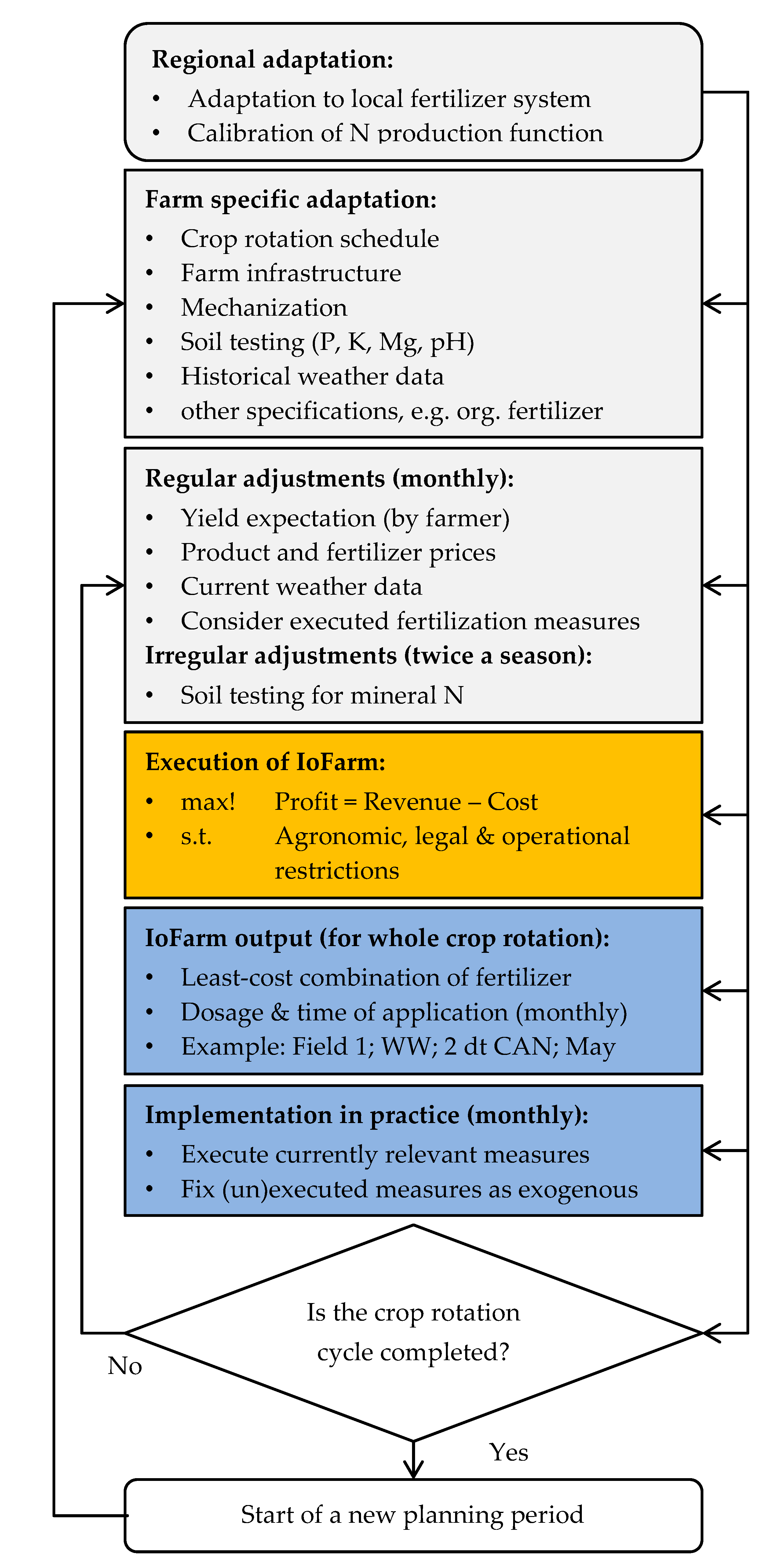
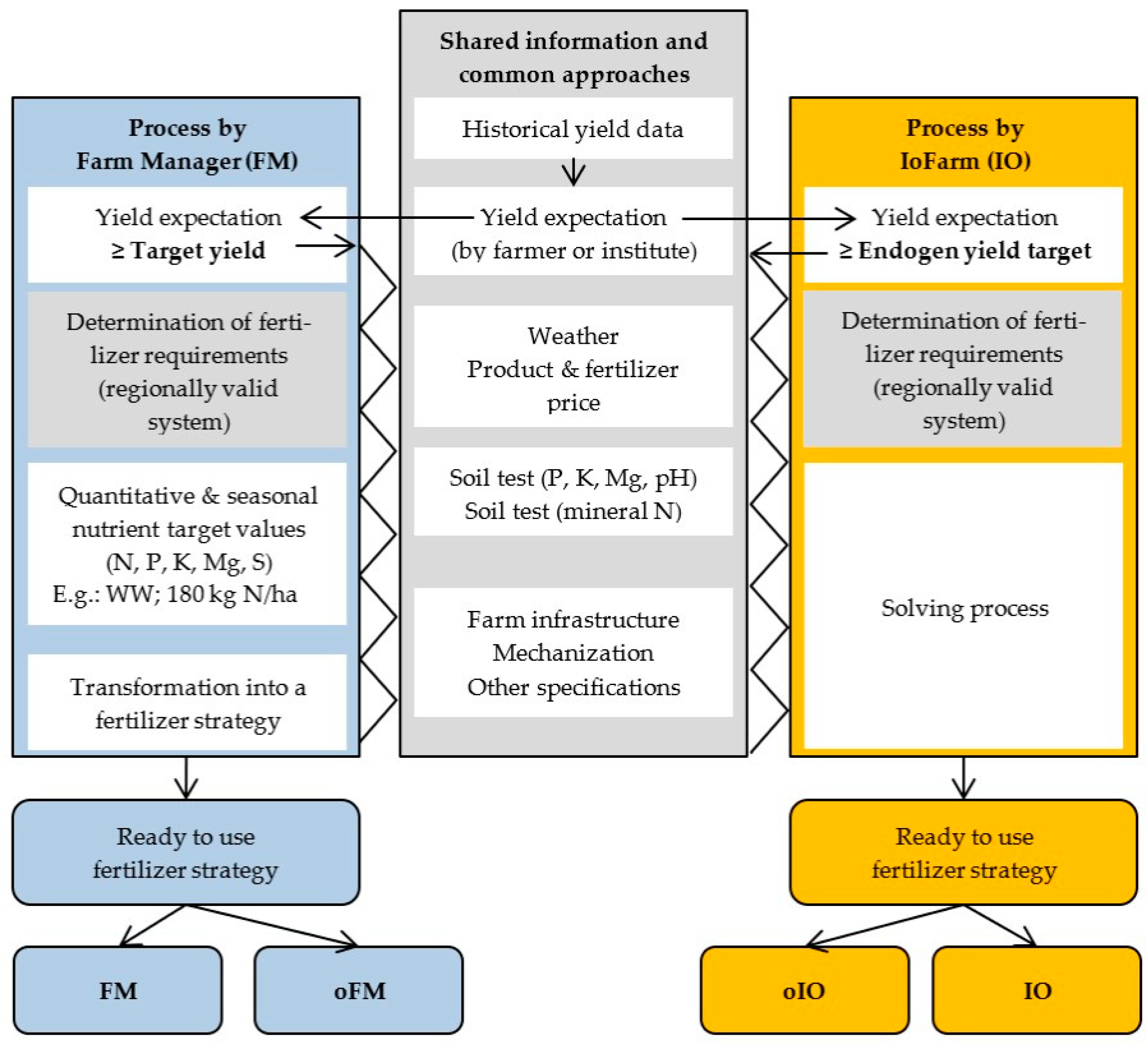
2.1. IoFarm Decision-Support System

IoFarm is a novel DSS to reduce fertilizer expenditure on the farm level [1]. The system provides precise guidance on fertilizer selection, application rate, and application timing for each field plot over an entire crop rotation cycle. Through regular updates of fertilizer and product prices, yield expectations, soil test results, and weather information, IoFarm is quickly adapted to changing conditions. To make the most of this ability, IoFarm should be used once a month during the growing season to recalculate the fertilization strategy. IoFarm falls into the category of mixed integer nonlinear problems. The objective function was designed to find the economically optimal fertilizer strategy that satisfies crop requirements. In addition to the market prices of the fertilizers, the application costs are also relevant in this choice. Within the model, marginal revenue and marginal cost are used to determine the optimal nutrient application, and hence yield level. Figure 1 provides a general overview of IoFarm’s data input, data processing, and output.

After this general overview of DSS IoFarm, some information on how IoFarm works and how it incorporates data from the biophysical environment is summarized below. The estimation of nitrogen dynamics in the soil is performed with the help of two annual soil tests, soil temperature and climatic water balance (CWB). The first soil test is performed in spring at the beginning of the growing season or before the first fertilization. The second soil test is carried out after harvest. Soil nitrogen content between these two sampling dates is derived from soil temperature (nitrogen mineralization) and CWB (leaching of nitrogen). Both of these measurements are typically recorded by local weather stations, and are therefore available as long-term monthly averages for forecasting purposes. Long-term monthly averages are replaced month by month by actual measured values. This approach to estimate nitrogen dynamics is highly simplified. It can only be justified by regular updates with real measured values for soil nitrogen content and by prioritizing a high level of user friendliness. Scientific models such as HERMES [19], WAVE [20], DAISY [21], or MONICA [22] are available, but they are too complex for use in the context of a practical DSS. To determine the crop-specific nutrient requirements of N, P, K, Mg, and S, IoFarm must be adapted and calibrated to regionally common methods. This means that IoFarm is not an independent fertilizer system, but is based on the specifications of an externally specified fertilizer system, which is required in many countries for legal reasons. IoFarm could be said to just be a problem solver for a given fertilizer system. For the field trial, IoFarm was adapted to the usual nutrient requirement calculation of the trial sites. All three sites were located in Bavaria (southern Germany), so the calculation of requirements in our case was based on the guidelines of the Bavarian State Institute for Agriculture [23].

We now present the basic features of this fertilizer system. The system is based on site-specific yield expectations, which are defined by the farmer or through statistical data. From this, the fertilizer requirement of the nutrients is derived. For nitrogen, the soil supply of available mineral nitrogen at the beginning of the season is deducted. Standard values offer the possibility of taking into account, for example, crop development or N mineralization with additions and deductions. The fertilizer requirement of nutrients P, K, and Mg is also adjusted depending on the location. This is conducted on the basis of soil-test results. If the respective nutrient content is low, additions are applied; the same applies in reverse for high nutrient contents. As a result, this system of determining fertilizer requirements provides information on the quantities of nutrients that can be used per hectare and year. The farmer uses this information to form their own fertilization strategy.

IoFarm largely follows this fertilization system, but additionally calculates an economically optimized fertilization strategy. It is taken into account that fertilization measures can also take place aggregated, in the course of a crop rotation (e.g., potash fertilization). IoFarm differs from the fertilization system described above only in the determination of N requirements. As already described above, nitrogen dynamics in the soil are taken into account in a simplified form within the model. In combination with fertilization, which is also internally determined in the model, it is thus known which N content is available to the plants month by month from the soil. Nitrogen must be allocated to the plants as close as possible to their temporal requirements. In order to account for this, the percentage nitrogen uptake of plants at distinctive developmental stages is estimated on the basis of literature data [24,25,26]. In combination, this enables the identification of when and to what extent nitrogen fertilization is required. As crop-yield response function, IoFarm uses a linear function with different slopes depending on the nutrient. The maximum of this function is limited by the yield expectation of the farmers. In summary, the following applies: IoFarm is designed to meet important crop-management requirements for fertilization. An attempt is made to model the nitrogen dynamics in the soil and to synchronize fertilizer application as optimally as possible with the nutrient requirements of the plants over the growing season and the entire crop rotation. This ensures balanced nutrition and avoids overdosing of nutrients. For further details, please refer to the original manuscript [1].

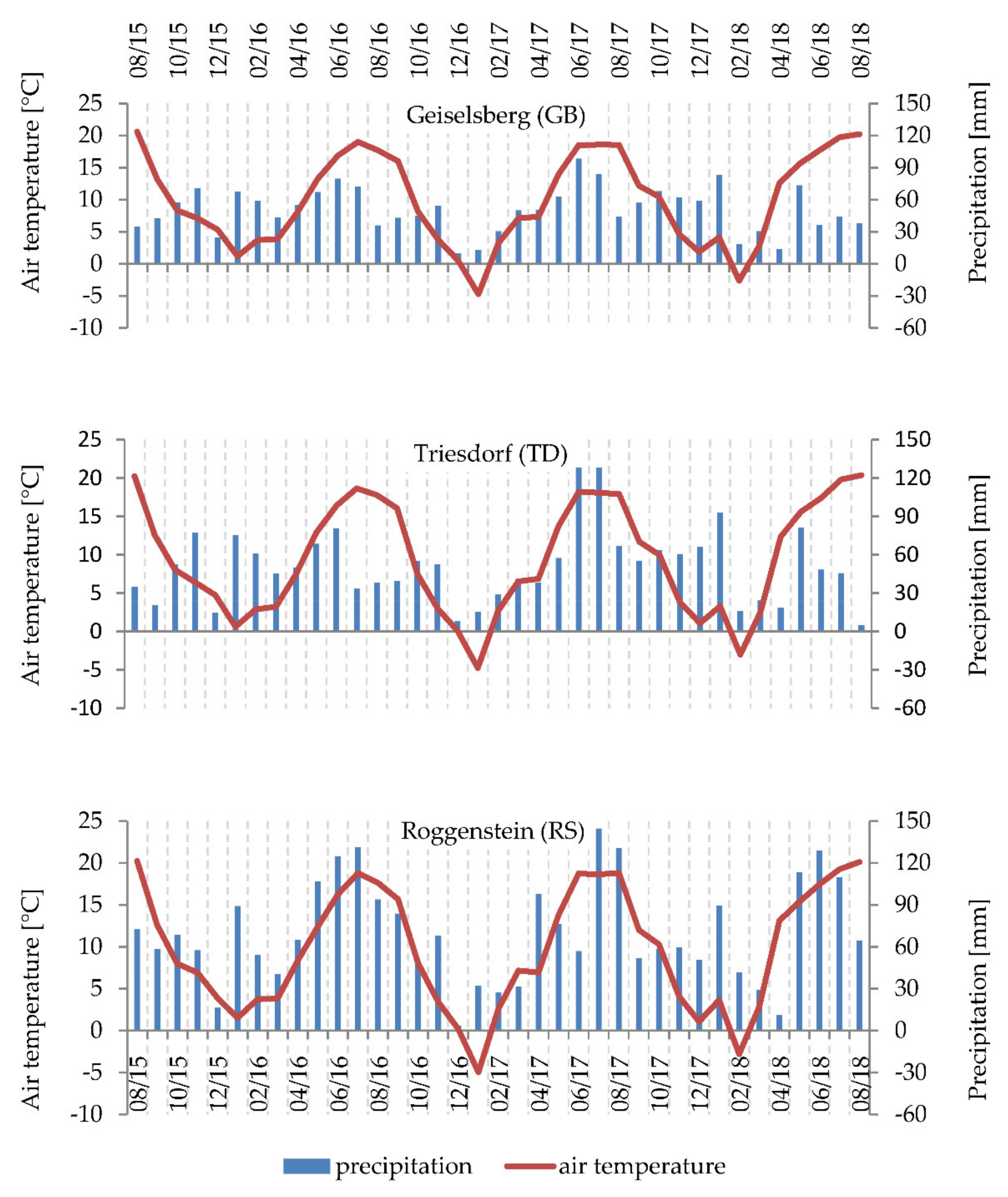
2.2. Site Description and Weather Conditions

The field experiment was conducted over three crop years (2016 to 2018) and at three locations within Bavaria (southern Germany): Geiselsberg (GB; 49°08′ N, 10°50′ E; altitude, 505 m), Triesdorf (TD; 49°11′ N, 10°39′ E; altitude, 430 m), and Roggenstein (RS; 48°11′ N, 11°20′ E; altitude, 514 m). The soil properties at the beginning of the experiment are shown in

Table 1. Soil properties of three field sites in Bavaria.

Site		GB			TD			RS
Plots		{1, … 9}	{10, … 18}	{18, … 27}	{1, … 15}	{16, … 30}	{31, … 45}	{1, … 9}	{10, … 18}	{19, … 27}
Soil type		Cambisol			Planosol			Cambisol
Soil texture		Loam			Sandy Loam			Silty Clay
Soil pH		6.6	6.6	6.9 *	7.3 *	7.3 *	7.3 *	6.1	6.0	6.0
Usable field capacity %		17.5	16.2	16.2	12.7	15.5	16.0	24.5	21.8	23.7
Bulk density	g cm−3	1.25	1.27	1.29	1.24	1.33	1.35	1.43	1.45	1.50
Organic matter	%	2.1	2.2	2.9	2.5	2.6	2.4	1.7	1.7	1.7
P2O5	mg100 g−1	12	6	8	17	19	24	7	7	7
K2O	mg100 g−1	36	28	22	17	18	19	14	15	16
MgO	mg100 g−1	9	6	7	20	19	18	4	5	3

* Soil pH is above the desired level, therefore no liming was allowed.

.

Weather records are based on data from the nearest weather stations (Windsfeld, Triesdorf, and Roggenstein) of the German Weather Service [27]. Our own precipitation records were used for GB, as deviations were expected due to a distance of about 8000 m to the nearest weather station. Figure 2 provides a selection of relevant weather information.

2.3. Field Experiment

The experiment was set up in a two-factorial design with three locations and three crop years. The first factor reflected the fertilization variant and was composed of a farm manager variant (FM), an IoFarm variant (IO), and a control variant (0V) without any fertilization. Additional organic fertilizer in the form of digestate was integrated into the trial at the TD site. Here, additional organomineral variants were created (oFM, oIO). The second factor was formed by different crops that were grown at each site in each year: winter wheat (WW; Triticum aestivum L.), silage maize (SM; Zea mays L.), and winter barley (WB; Hordeum vulgare L.). As both plots and variants were fixed over the entire experimental period, the experiment replicated a complete crop rotation cycle on each plot. The experiment was planned in a split-plot design with randomized replications. In GB and TD, the plots were laid out at 12 × 4.5 m, and the crop was harvested in a core area of 9 × 1.38 m for cereals, and 9 × 1.5 m for SM. Due to the different technology, the plot size in RS was 10 × 6 m. Here, the core area was harvested at 10 × 1.56 m for cereals and 10 × 1.5 m for SM. In RS, fertilizer was applied using a lifted drill. However, in GB and TD, fertilizers were applied using a plot spreader with a belt-head dispenser (own construction of the Educational Schools Triesdorf, Weidenbach, Germany). Digestate was only applied in TD using a slurry tank with a trailing shoe applicator (Gülle Zwerg constructed by Zunhammer in Traunreut, Germany), which was specially developed for plot trials. Digestate was applied according to a target in m³ ha⁻¹. The maximal available amount of digestate was limited to 4000 m³ per year for the assumed farm area of 150 ha. Repeated analysis of the digestate served to update the nutrient content.

Figure 3 presents how the tested fertilizer variants (FM, oFM, IO, oIO) were created. Both the farm managers and IoFarm used the same information.

Process by farm manager (Figure 3, left column): For the experiment, a yield expectation was assigned to each crop by the local farm managers. This value was based on empirical values (historical yield data). Subsequently, nutrient requirements were calculated for nitrogen, phosphorus, potash, and magnesium according to specifications of the Bavarian State Institute for Agriculture [23]. A description of this fertilizer system can be found in Section 2.1. The calculated quantitative and seasonal nutrient target values were passed on to the farm managers together with current fertilizer prices and other shared information. Then, with the help of a planning tool, the farm managers defined a ready-to-use fertilizer strategy for all three crops (For more information on the used planning tool, please refer to the following link: https://drive.google.com/file/d/14rBHNKKDuBq8oyeeVUXuek2id1B9z_Dw/view?usp=sharing, accessed on 20 June 2021). The objective of the exercise was to select the most cost-effective option from the available fertilizers while satisfying the specified nutrient demands as much as possible. For phosphorus, potash, and magnesium, fertilization was freely allocable within crop rotation. However, lime fertilizers could not be applied to areas with a pH value above the site-specific optimum (compare Table 1). In the case of a fertilizer application, a minimal rate of 300 kg ha⁻¹ was specified for lime fertilizer, 12.5 m³ ha⁻¹ for digestate, and 80 kg ha⁻¹ for all other fertilizers. As application costs also play a role in fertilizer strategy selection, a hypothetical farm was specified with 50 ha of WW, 50 ha of WB, and 50 ha of SM. The average field-to-farm distance was set as 7 min. Although this information is irrelevant to the evaluated parameters in this experiment, it is important for determining a particular fertilizer strategy, and is thereby mentioned here. This is how farm managers’ mineral and organomineral fertilizer variants (FM and oFM) were generated. This procedure was repeated monthly, starting from the fall sowing season in 2015. The shared information, such as results from soil N_min testing and price changes, was constantly updated. Thus, farm managers had the opportunity to adjust their target yield and fertilizer strategy once a month at the beginning of the application period before the fertilizers were applied. However, the possibility to adjust the target yield was rarely used by the farm managers during the trial period. An overview of N_min values and adjustments to yield expectations can be found in Appendix A (

Table A2. Results from soil testing (N_min) and farmers’ yield expectation (YEX).

Site →	Geiselsberg			|	Triesdorf					|	Roggenstein
Variant →	IO	FM		|	IO	FM	oIO	oFM		|	IO	FM
Crop and	Nmin	Nmin	YEX **	|	Nmin	Nmin	Nmin	Nmin	YEX **	|	Nmin	Nmin	YEX **
Date ↓	kg ha−1		dt ha−1	|	kg ha−1		kg ha−1		dt ha−1	|	kg ha−1		dt ha−1
Winter Barley				|						|
02/2016	41	41	75	|	46	46	46	46	75	|	26	26	80
04/2016			75	|					70	|			80
07/2016			H *	|					H *	|			H *
08/2016	82	83	75	|	65	69	72	67	75	|	62	74	80
02/2017	62	65	75	|	41	43	45	42	75	|	19	12	80
06/2017			70	|					70	|			75
07/2017			H *	|					H *	|			H *
08/2017	161	85	75	|	126	175	90	98	75	|	33		80
02/2018	39	44	75	|	31	33	34	35	75	|	23	23	80
07/2018			H *	|					H *	|			H *
Winter Wheat				|						|
02/2016	52	52	85	|	50	50	50	50	85	|	30	30	89
04/2016			85	|					70	|			89
08/2016	106	74	H *	|	49	41	43	37	H *	|	24	21	H *
09/2016			85	|					85	|			89
02/2017	76	83	85	|	51	50	44	46	85	|	20	16	89
04/2017			85	|					80	|			89
06/2017			75	|					75	|			89
07/2017			H *	|					H *	|			H *
08/2017	108	116		|						|
09/2017			85	|					85	|			89
10/2017			85	|	64	60	62	56	85	|	67		89
02/2018	49	44	85	|	45	34	43	41	85	|	32	32	89
07/2018			H *	|					H *	|			H *
Silage Maize				|						|
04/2016	41	41	176	|	49	49	49	49	160	|	26	26	192
08/2016	89	95	176	|	91	85	95	92	160	|	50		192
09/2016			H *	|					H *	|			H *
03/2017	38	51	176	|	38	23	26	30	160	|	30	28	192
05/2017			176	|					160	|			176
08/2017	88	98	176	|	104	88	89	90	160	|			176
09/2017			H *	|					H *	|			H *
10/2017			176	|					160	|			192
03/2018	18	25	176	|	32	32	36	35	160	|	15	15	192
09/2018			H *	|					H *	|			H *

* Harvest; ** farmers yield expectation in dt ha⁻¹ (1 dt = 100 kg). Only months in which new information or changes occurred compared to the previous month are shown. Changes highlighted in bold.

).

Process by IoFarm (Figure 3, right column): Fertilization variants IO and oIO were defined with the help of IoFarm. The endogenous yield target of IoFarm was also limited by yield expectation (updated monthly by farm manager). Again, this was followed by determining the fertilizer requirement and the solving process in which IoFarm calculates the economically optimal fertilizer strategy. Regular updates of the input parameters (shared information) also require a regular repetition of this procedure.

Externally defined yield expectation has great influence on the intensity of fertilization in this system. Reliable yield prediction requires a lot of experience and is only possible relatively late in the growing season. Incorrect predictions lead to biases, but can probably be minimized, by integrating a validated plant-growth model into IoFarm in future. For the sake of usability and comparability, however, we decided to work with the farmers’ yield expectation. This approach is quite common and is also used by extension services to achieve a regional differentiation of nutrient supply [28].

2.4. General Cultivation Management

To begin the trial in the first year with a neutral preceding crop, winter oilseed rape was grown in the preceding year in GB and TD. In RS, the preceding crop was spring barley. The soil was tilled with a cultivator, which was used several times if required. A rotary harrow was used to prepare the seedbed. Before sowing SM, an intercrop mixture (25 kg ha⁻¹ “Terra Life Aqua pro”) was sown in summer. The following seeding information applies to the main crops:

• WB: 320 tsr m⁻², KWS Meridian variety approx. 25 September, drill sowing.
• WW: 340 tsr m⁻², Patras variety, approx. 5 October, drill sowing.
• SM: 9 tsr m⁻², P8589 variety, approx. 25 April, precision seeding, row width 75 cm.

The used varieties are standard regional varieties. Plant protection measures were adapted to the conditions of the respective locations. Weed control was very successful. Fungicide and insecticide measures in the cereals were designed to keep the plants completely healthy. In the first year of cultivation, notable Ramularia infections of WB appeared at the RS site, and slight Septoria tritici infections of WW were detected at the GB site. Otherwise, disease and pest control was very successful. Fertilization measures were extremely diverse across all sites, crops, and varieties. An overview of all measures, including fertilizer choice, can be found in

Table A1. Detailed documentation of fertilizer application in dt per hectare (1 dt = 100 kg).

Geiselsberg: 2016			|	IO			|		|	FM
		Fertilizer Code *	|	SM	WB	WW	|	Fertilizer Code	|	SM	WB	WW
Mar	|	12: 18,46,0,0,0, −36	|		2.6		|	02: 27,0,0,4,0, −9	|		2.5	2.5
	|	21: 0,0,40,6,5,0	|		3.3		|		|
	|	26: 0,0,0,14,0,53	|		3.0		|		|
Apr	|	12: 18,46,0,0,0, −36	|			1.8	|	02: 27,0,0,4,0, −9	|		1.0
	|	24: 0,0,0,25,20,0	|			0.8	|	19: 0,0,46,0,0, −1	|		2.5
	|	04: 46,0,0,0,0, −46	|		1.2		|	07: 21,0,0,0,24, −63	|			1.5
	|		|				|	12: 18,46,0,0,0, −36	|			2.0
May	|	04: 46,0,0,0,0, −46	|	2.1		1.7	|	02: 27,0,0,4,0, −9	|		2.0
	|	21: 0,0,40,6,5,0	|		1.4	4.7	|	04: 46,0,0,0,0,−46	|	3.0
	|	12: 18,46,0,0,0, −36	|	2.4	2.6		|	12: 18,46,0,0,0,−36	|	2.0
	|	07: 21,0,0,0,24, −63	|	0.8			|		|
	|	25: 0,0,0,0,2,50	|	3.0			|		|
	|	26: 0,0,0,14,0,53	|	6.1			|		|
Jun	|	04: 46,0,0,0,0, −46	|			1.1	|	02: 27,0,0,4,0,−9	|			2.0
Jul	|	12: 18,46,0,0,0, −36	|			1.1	|		|
Geiselsberg: 2017			|	IO			|		|	FM
		Fertilizer Code *	|	SM	WB	WW	|	Fertilizer Code *	|	SM	WB	WW
Aug		19: 0,0,46,0,0, −1	|		2.9	4.5	|		|
Oct		26: 0,0,0,14,0,53	|	3.0	3.0		|		|
Nov			|				|	26: 0,0,0,14,0,53	|	6.0	6.0
Mar		02: 27,0,0,4,0, −9	|			1.3	|	02: 27,0,0,4,0,−9	|	2.5
		21: 0,0,40,6,5,0	|		0.8	0.8	|	19: 0,0,46,0,0,−1	|	1.5
		24: 0,0,0,25,20,0	|			0.8	|	13: 20,20,0,0,0,−31	|			3.5
Apr		07: 21,0,0,0,24, −63	|	1.0			|	13: 20,20,0,0,0,−31	|			3.5
		02: 27,0,0,4,0, −9	|			2.5	|	02: 27,0,0,4,0,−9	|	2.0
			|				|	21: 0,0,40,6,5,0	|		2.0
May		04: 46,0,0,0,0, −46	|	2.0	3.0		|	02: 27,0,0,4,0,−9	|	1.0
		12: 18,46,0,0,0, −36	|	2.5			|	04: 46,0,0,0,0,−46	|		2.0
		02: 27,0,0,4,0, −9	|			2.1	|	12: 18,46,0,0,0,−36	|		3.0
		07: 21,0,0,0,24,−63	|		0.9		|		|
Geiselsberg: 2018			|	IO			|		|	FM
		Fertilizer Code *	|	SM	WB	WW	|	Fertilizer Code *	|	SM	WB	WW
Mar		04: 46,0,0,0,0, −46	|		1.5		|	02: 27,0,0,4,0,−9	|	2.5	3
		12: 18,46,0,0,0, −36	|		2.4		|	12: 18,46,0,0,0,−36	|	2
		04: 46,0,0,0,0, −46	|	2			|	26: 0,0,0,14,0,53	|	3
		07: 21,0,0,0,24, −63	|	0.8			|	19: 0,0,46,0,0,−1	|		5
		12: 18,46,0,0,0, −36	|	0.8			|	22: 0,0,40,6,5,0	|		5
		26: 0,0,0,14,0,53	|	3.7			|	24: 0,0,0,25,20,0	|		1.5
Apr		07: 21,0,0,0,24, −63	|		0.8		|	04: 46,0,0,0,0,−46	|			1.7
		26: 0,0,0,14,0,53	|		7.3		|	12: 18,46,0,0,0,−36	|			4.5
		02: 27,0,0,4,0, −9	|			4.7	|	21: 0,0,40,6,5,0	|			5
		12: 18,46,0,0,0, −36	|			2.2	|	26: 0,0,0,14,0,53	|			13
May		04: 46,0,0,0,0, −46	|	0.8	1.3		|	02: 27,0,0,4,0,−9	|	2.3	2.5
		21: 0,0,40,6,5,0	|		1.2		|		|
		24: 0,0,0,25,20,0	|			2.9	|		|
Jun			|				|	02: 27,0,0,4,0,−9	|		1.5
Triesdorf: 2016			|	IO			|		|	FM
		Fertilizer Code *	|	SM	WB	WW	|	Fertilizer Code *	|	SM	WB	WW
Mar		04: 46,0,0,0,0, −46	|		1.3	0.8	|	15: 15,15,15,0,2,−15	|			4.0
		12: 18,46,0,0,0, −36	|		0.8		|	17: 23,5,5,0,6,−23	|		2.5
		21: 0,0,40,6,5,0	|		4.8		|		|
Apr		21: 0,0,40,6,5,0	|	8.4		5.6	|	04: 46,0,0,0,0,−46	|	2.5
		12: 18,46,0,0,0, −36	|		0.9		|	12: 18,46,0,0,0,−36	|	2.0
			|				|	06: 26,0,0,0,13,−49	|		2.0
May		04: 46,0,0,0,0, −46	|	2.1		0.8	|	06: 26,0,0,0,13,−49	|			1.5
		12: 18,46,0,0,0, −36	|	3.6	0.8	1.4	|		|
Jun		04: 46,0,0,0,0, −46	|			1.1	|	06: 26,0,0,0,13,−49	|		2.0	2.7
Jul		12: 18,46,0,0,0, −36	|		2.2		|		|
Triesdorf: 2017			|	IO			|		|	FM
		Fertilizer Code *	|	SM	WB	WW	|	Fertilizer Code *	|	SM	WB	WW
Feb		21: 0,0,40,6,5,0	|	1.6	0.8		|		|
Mar		02: 27,0,0,4,0, −9	|	1.1		2.5	|	05: 24,0,0,0,6,−34	|	2.5
			|				|	20: 0,16,16,2,7,6	|	5.0		4.0
			|				|	18: 23,5,5,0,6,−23	|			2.5
Apr		11: 9,0,0,0,0, −9	|	2.4			|	05: 24,0,0,0,6,−34	|	2.0		1.5
		02: 27,0,0,4,0, −9	|			2.1	|		|
		21: 0,0,40,6,5,0	|			2.4	|		|
May		02: 27,0,0,4,0, −9	|	1,6	1.6	1.7	|	02: 27,0,0,4,0,−9	|	3.0
		07: 21,0,0,0,24, −63	|	0.8	0.8	0.8	|	05: 24,0,0,0,6,−34	|			2.5
		11: 9,0,0,0,0, −9	|	2.3			|	04: 46,0,0,0,0,−46	|		3.0
		12: 18,46,0,0,0, −36	|	1.4	0.8		|	12: 18,46,0,0,0,−36	|		1.0
		04: 46,0,0,0,0, −46	|		1.8		|		|
Jun		11: 9,0,0,0,0, −9	|	1.1			|		|
Triesdorf: 2018			|	IO			|		|	FM
		Fertilizer Code *	|	SM	WB	WW	|	Fertilizer Code *	|	SM	WB	WW
Mar		02: 27,0,0,4,0, −9	|		1.4		|	05: 24,0,0,0,6,−34	|	2.5
		04: 46,0,0,0,0, −46	|	3.9	1.0		|	20: 0,16,16,2,7,6	|	1.7
		24: 0,0,0,25,20,0	|	0.9			|	22: 0,0,40,6,5,0	|	3.7	6.4
			|				|	06: 26,0,0,0,13,−49	|		2.5
			|				|	19: 0,0,46,0,0,−1	|		3.6
			|				|	24: 0,0,0,25,20,0	|		2.0
Apr		02: 27,0,0,4,0, −9	|		1.0	1.8	|	14: 15,5,20,2,8,−14	|	8.0	10.0
		24: 0,0,0,25,20,0	|		0.8		|	24: 0,0,0,25,20,0	|	1.3		1.8
		04: 46,0,0,0,0, −46	|			1.7	|	04: 46,0,0,0,0,−46	|			3.5
		07: 21,0,0,0,24, −63	|			0.8	|	22: 0,0,40,6,5,0	|			5.8
		12: 18,46,0,0,0, −36	|			1.2	|		|
		21: 0,0,40,6,5,0	|			1.2	|		|
May		04: 46,0,0,0,0, −46	|		1.1		|		|
		12: 18,46,0,0,0, −36	|		0.9		|		|
		21: 0,0,40,6,5,0	|		7.4		|		|
Jun		02: 27,0,0,4,0, −9	|		0.8		|		|
Roggenstein: 2016			|	IO			|		|	FM
		Fertilizer Code *	|	SM	WB	WW	|	Fertilizer Code *	|	SM	WB	WW
Mar		04: 46,0,0,0,0, −46	|		0.8	2.3	|	12: 18,46,0,0,0,−36	|		3	4
		07: 21,0,0,0,24, −63	|		0.8		|	24: 0,0,0,25,20,0	|		0.5	0.5
		12: 18,46,0,0,0, −36	|		0.8	1	|		|
		26: 0,0,0,14,0,53	|		5.5	4.1	|		|
		21: 0,0,40,6,5,0	|			2.8	|		|
Apr		26: 0,0,0,14,0,53	|	5.1			|	02: 27,0,0,4,0,−9	|			2.6
May		04: 46,0,0,0,0, −46	|	3.3	1.2		|	02: 27,0,0,4,0,−9	|		3.1	1.7
		12: 18,46,0,0,0, −36	|	4	0.8	0.8	|	04: 46,0,0,0,0,−46	|	2.5
		21: 0,0,40,6,5,0	|	8.4	1.5	1.8	|	12: 18,46,0,0,0,−36	|	3
			|				|	21: 0,0,40,6,5,0	|	10
			|				|	26: 0,0,0,14,0,53	|	10
Jun		12: 18,46,0,0,0, −36	|		1.6	2.3	|	02: 27,0,0,4,0,−9	|		3.2
Jul		03: 28,0,0,0,0, −28	|		1.7		|		|
Sep			|				|	26: 0,0,0,14,0,53	|		12	12
Roggenstein: 2017			|	IO			|		|	FM
		Fertilizer Code *	|	SM	WB	WW	|	Fertilizer Code *	|	SM	WB	WW
Feb		21: 0,0,40,6,5,0	|	1.9	0.8		|		|
Mar		02: 27,0,0,4,0, −9	|	2.8			|	02: 27,0,0,4,0,−9	|	2.2	2.2
		26: 0,0,0,14,0,53	|	4.7		8.6	|		|
		03: 28,0,0,0,0, −28	|		5.7		|		|
Apr		11: 9,0,0,0,0, −9	|		0.8		|	01: 27,0,0,0,0,−15	|	2.8
		26: 0,0,0,14,0,53	|		10		|	10: 46,0,0,0,0,−46	|			2.5
		07: 21,0,0,0,24, −63	|			1.1	|	07: 21,0,0,0,24,−63	|	1.5	1
		10: 46,0,0,0,0, −46	|			2.7	|	12: 18,46,0,0,0,−36	|	3	3	2.5
		12: 18,46,0,0,0, −36	|			2.1	|	22: 0,0,40,6,5,0	|			10
May		04: 46,0,0,0,0, −46	|	1.2			|	01: 27,0,0,0,0,−15	|		2
		07: 21,0,0,0,24, −63	|	0.8	0.8		|		|
		12: 18,46,0,0,0, −36	|	3.1	2.5		|		|
Jun		12: 18,46,0,0,0, −36	|	0.8			|		|
Roggenstein: 2018			|	IO			|		|	FM
		Fertilizer Code *	|	SM	WB	WW	|	Fertilizer Code *	|	SM	WB	WW
Mar		02: 27,0,0,4,0, −9	|	1.1		1	|	06: 26,0,0,0,13,−49	|	2.5		2.3
		04: 46,0,0,0,0, −46	|	1.9		1.5	|		|
		12: 18,46,0,0,0, −36	|			2.7	|		|
		07: 21,0,0,0,24, −63	|	0.8			|		|
Apr		26: 0,0,0,14,0,53	|	4.5		3.2	|	01: 27,0,0,0,0,−15	|	1.2		1.4
		02: 27,0,0,4,0, −9	|		2		|	02: 27,0,0,4,0,−9	|	0.7
		04: 46,0,0,0,0, −46	|		2		|	12: 18,46,0,0,0,−36	|	3.5	3.7	2.3
		12: 18,46,0,0,0, −36	|		3.6		|	26: 0,0,0,14,0,53	|	4.5
		21: 0,0,40,6,5,0	|		8.1		|	22: 0,0,40,6,5,0	|		11
May		04: 46,0,0,0,0, −46	|			1.5	|	01: 27,0,0,0,0,−15	|		3.5	2.9
		21: 0,0,40,6,5,0	|	0.8		5	|		|
		12: 18,46,0,0,0, −36	|	1.5			|		|
Triesdorf: 2016			|		oIO		|		|		oFM
		Fertilizer Code *	|	SM	WB	WW	|	Fertilizer Code *	|	SM	WB	WW
Mar		28: Digestate	|			13	|	05: 24,0,0,0,6,−34	|		2.5	2.5
		04: 46,0,0,0,0, −46	|		1.3		|		|
		21: 0,0,40,6,5,0	|	2.5	4.3		|		|
Apr		12: 18,46,0,0,0, −36	|		1.7		|	28: Digestate	|		18	22
May		07: 21,0,0,0,24, −63	|			0.8	|	07: 21,0,0,0,24,−63	|	2
		28: Digestate	|	48		20	|	28: Digestate	|	40
		04: 46,0,0,0,0, −46	|		1		|		|
		12: 18,46,0,0,0, −36	|	1.4			|		|
Jun		04: 46,0,0,0,0, −46	|			1	|	05: 24,0,0,0,6,−34	|		2	2
Triesdorf: 2017			|		oIO		|		|		oFM
		Fertilizer Code *	|	SM	WB	WW	|	Fertilizer Code *	|	SM	WB	WW
Mar		03: 28,0,0,0,0, −28	|	1.1		3.5	|	05: 24,0,0,0,6,−34	|	2.5		2.5
		28: Digestate	|	13			|	20: 0,16,16,2,7,6	|	5
Apr		28: Digestate	|	13	43	13	|	28: Digestate	|	25	35	20
May		07: 21,0,0,0,24, −63	|	0.8		0.8	|	12: 18,46,0,0,0,−36	|		1
		11: 9,0,0,0,0, −9	|	1.9		1.3	|	05: 24,0,0,0,6,−34	|	1		2
		12: 18,46,0,0,0, −36	|	0.8		0.8	|		|
		07: 21,0,0,0,24, −63	|		0.8		|		|
Jun		11: 9,0,0,0,0, −9	|	0.8			|		|
Triesdorf: 2018			|		oIO		|		|		oFM
		Fertilizer Code *	|	SM	WB	WW	|	Fertilizer Code *	|	SM	WB	WW
Mar		02: 27,0,0,4,0,−9	|		1.4		|	06: 26,0,0,0,13,−49	|	2
		04: 46,0,0,0,0,−46	|	2.8			|	19: 0,0,46,0,0,−1	|	0.8
		24: 0,0,0,25,20,0	|			0.8	|	05: 24,0,0,0,6,−34	|		2.5
			|				|	20: 0,16,16,2,7,6	|		5
			|				|	24: 0,0,0,25,20,0	|		2.2
Apr		28: Digestate	|	13	24	44	|	04: 46,0,0,0,0,−46	|			1.4
		04: 46,0,0,0,0,−46	|			1.3	|	02: 27,0,0,4,0,−9	|	1	1.5
			|				|	28: Digestate	|	20	20	40
			|				|	20: 0,16,16,2,7,6	|			1.2
			|				|	24: 0,0,0,25,20,0	|			1.5
May		02: 27,0,0,4,0,−9	|		2.2		|	02: 27.0.0.4.0.−9	|	2
		12: 18,46,0,0,0,−36	|		0.8		|	15: 15,15,15,0,2,−15	|		4
		24: 0,0,0,25,20,0	|		1.3		|		|
		07: 21,0,0,0,24,−63	|	0.8			|		|
Jun		12: 18,46,0,0,0,−36	|		1.7		|		|

* First two digits of fertilizer codes are used to assign the fertilizer. Colon is followed by the respective composition of the fertilizers with the nutrient contents for N, P₂O₅, K₂0, MgO, S, and their CaO effects. Fertilizers: 01, 02, and 05 = CAN, 03 = ammonium nitrate urea solution, 04 and 08 = urea, 06 = ammonium sulfate nitrate; 07 = sulfuric acid ammonia, 09 = ENTEC26, 10 = stabilized urea, 11 = ammonium nitrate urea solution + water, 12 = DAP, 13 = NP; 14 = ENTEC NPK, 15 to 18 = NPK, 19 = TSP, 20 = PK, 21 and 22 = potash, 23 = kainite, 24 = kieserit, 25 to 27 = lime, 28 = digestat. Variants: IO = IoFarm, FM = farm manager, oIO = IO + digestate, oFM = FM + digestate.

in Appendix A. For a detailed differentiation of the fertilizer strategies themselves, we refer to [29]. To obtain an overview of the quantities of applied nutrients, individual measures are also summarized and compared in Section 3.1 (

Table 2. Comparative overview of nutrient supply by location, crop, and treatment.

Site:	Geiselsberg		Roggenstein		Triesdorf		Triesdorf
Treatment:	FM	IO	FM	IO	FM	IO	oFM	oIO
Silage maize
N + Nmin	199	193	186	231	190	199	196	209
P2O5	146	116	140	149	46	85	72	80
K2O	93	11	407	219	77	138	167	220
MgO	100	74	108	99	27	25	44	48
S	12	36	48	34	22	27	38	25
Winter barley
N + Nmin	201	204	188	211	206	209	217	223
P2O5	116	161	161	125	52	71	37	52
K2O	0	73	0	83	141	95	81	109
MgO	28	57	92	103	27	30	19	15
S	5	19	22	22	90	22	31	21
Winter wheat
N + Nmin	235	234	247	242	236	220	234	190
P2O5	130	122	127	151	119	58	102	70
K2O	67	79	0	111	199	194	167	65
MgO	73	67	73	84	43	44	44	28
S	30	28	25	26	105	34	70	25
Total crop rotation
N + Nmin	212	210	207	228	211	210	216	207
P2O5	131	133	143	142	72	71	70	67
K2O	53	54	136	138	139	143	138	132
MgO	67	66	91	95	32	33	36	30
S	16	28	32	27	72	28	46	24

All average values in kg ha⁻¹. FM = farm manager; IO = IoFarm; oFM and oIO were additionally treated with organic fertilizer. N + N_min = nitrogen fertilization + soil nitrogen content (soil test in spring).

). Cereal plots were harvested using plot combines (Haldrup c65, Ilshofen Germany). In GB and TD, SM plots were harvested using a two-row plot chopper equipped with rear container and weighing device. In RS, two maize rows were harvested by hand and then processed on-site with the above-mentioned plot chopper. Straw from the cereal plots remained on the harvested plots, and was afterwards chopped and incorporated. This procedure was repeated for three consecutive years until the crop rotation of WB-SM-WW was completed on each plot.

2.5. Crop and Soil Analysis

In fall 2015, detailed analysis of the soil conditions was conducted. All plots were analyzed for phosphorus, potash, magnesium, pH, organic matter, and soil type using standard methods, including calcium-acetate-lactate extraction. In parallel, nine undisturbed soil samples were collected at each site and analyzed for pore volume in the soil laboratory. Soil samples were annually taken at the beginning of the growing season or shortly before sowing SM to a depth of 0 to 30 cm and 30 to 60 cm to determine the supply of mineral nitrogen (N_min). This was separately performed for all variants. The results of the soil tests for mineral nitrogen only slightly differed among variants (Table A2 in Appendix A). In WB and WW, yield structure was also surveyed (for details see Section 3.5). Samples of the harvested material from WW and WG were analyzed for water and protein content using near-infrared spectroscopy (Perten DA 7250, PerkinElmer, Waltham, MA). In the case of SM, only dry matter was determined. For this purpose, 200 g samples were taken from each plot and dried for 24 h at 105 °C in a drying oven.

2.6. Statistical Analysis

Statistical analysis was performed using STAT software [30]. The two-factorial experiment (fertilization, crop) was evaluated using ANOVA for different dependent variables. In the case of significant F tests, multiple Tukey’s post hoc tests were performed for primary-factor fertilization to determine statistical differences. The Tukey test was chosen because it corrects for alpha error accumulation and is considered to be moderate. The prerequisites of ANOVA were confirmed using the Shapiro–Wilk test to check for normal distribution of residuals, and Levene’s test to check for homoscedasticity. In some groups, the data were not normally distributed (p < 0.05). However, with a sufficient number of observations per group (central-limit theorem), split-plot ANOVA was considered to be robust to the violation of this condition of a normal distribution of residuals [31]. Partial heteroscedasticity was also found. Various approaches used to transform the variables were inconclusive. The resulting consequences are discussed in Section 4, but they are not relevant to the post hoc tests that were performed.

ANOVA for the dependent variable yield (Y) was performed using Equation (1).

$$Y_{ijk}=\mu +f_i+r_k+e{(F)}_{ik}+c_j+{(fc)}_{ij}+e{(FC)}_{ijk}$$

(1)

where f represents the i-th effect of fertilization, r represents the effect of the k-th replicate, and e(F) represents the associated ik-th error term. Variable c represents the j-th effect of crop, fc is the effect of the interaction of fertilization and crop in the ij-th combination, and e(FC) is the ijk-th error term. Random effects are indicated with capital letters.

In addition to yield, variance analyses were also performed for other dependent variables. Equation (1) was adjusted accordingly:

$$P_{ijk}=\mu +f_i+r_k+e{(F)}_{ik}+c_j+{(fc)}_{ij}+e{(FC)}_{ijk}$$

(2)

$$M{P}_{ijk}=\mu +f_i+r_k+e{(F)}_{ik}+c_j+{(fc)}_{ij}+e{(FC)}_{ijk}$$

(3)

$$Y\_S{M}_{ik}=\mu +f_i+r_k+e{(F)}_{ik}$$

(4)

where the dependent variables from Equations (2)–(4) correspond to: (i) the protein content (P) of WB and WW; (ii) market performance (MP) taking into account the quality rating of WW; and (iii) the yield of each crop, here substituting Y_SM for SM. The underlying values of the variable MP are not measured, but were formed according to Equation (5).

$$M{P}_{c,t,pl}=y_{c,t,pl}\times P{y}_{c,t}$$

(5)

where y represents the yield of the c-th crop in the t-th year on the pl-th plot. Py represents the crop- and year-specific price, which, in the case of wheat, additionally depends on protein content.

3. Results

The basis for the interpretation of the results is a comparison of the nutrient supply of the test variants (Table 2). Results themselves show the influence of the IoFarm DSS on yield, quality, and market performance compared with the standard fertilizer strategy of a farm manager. Only marginal differences were found.

3.1. Comparison of Nutrient Supply and Fertilizer Use

As Table 2 shows, the site-specific nutrient supply of the test variants only slightly differed.

Larger deviations were found in the nitrogen fertilization of winter barley and silage maize at the Roggenstein site because of the different nitrogen sources: CAN was mainly used in the FM variant, while urea dominated in the IO variant due to relative price advantages. The higher gaseous losses of urea were taken into account by IoFarm through increased nitrogen fertilization. However, the emission targets of the European Union include a reduction in ammonia emissions [32]. In this context, urea fertilization is problematic and could possibly be further restricted. There were also major differences in the nitrogen supply to wheat in the oFM and oIO variants. Here, significantly less nitrogen was applied in the oIO variant. In contrast to the oFM variant, in the oIO variant, organic fertilization in wheat was divided into two applications in two out of three years, whereby better nitrogen utilization of the organic fertilization could be assumed. Further deviations can be seen in the sulfur fertilization at the Triesdorf site. Here, fertilization in the FM variant was above the requirements, perhaps because of the complexity of the optimization problem itself. The farm manager had difficulties in defining a fertilization strategy in which all nutrients were applied in sufficient quantities.

The most important nitrogen fertilizer by volume in the IO variant was urea at all sites (39% to 52% of total N fertilization). In FM variants, farm managers relied on different nitrogen fertilizers, including CAN (GB and TD_oFM), DAP (RS), and urea (TD_FM). Phosphate supply was predominantly provided by DAP, while TSP or PK 16 + 16 was used to a greater extent at only two sites in the FM variant. Potash supply took place almost entirely with grain potash. For more detailed analysis of the fertilizer strategy of IoFarm, a separate study is planned [29].

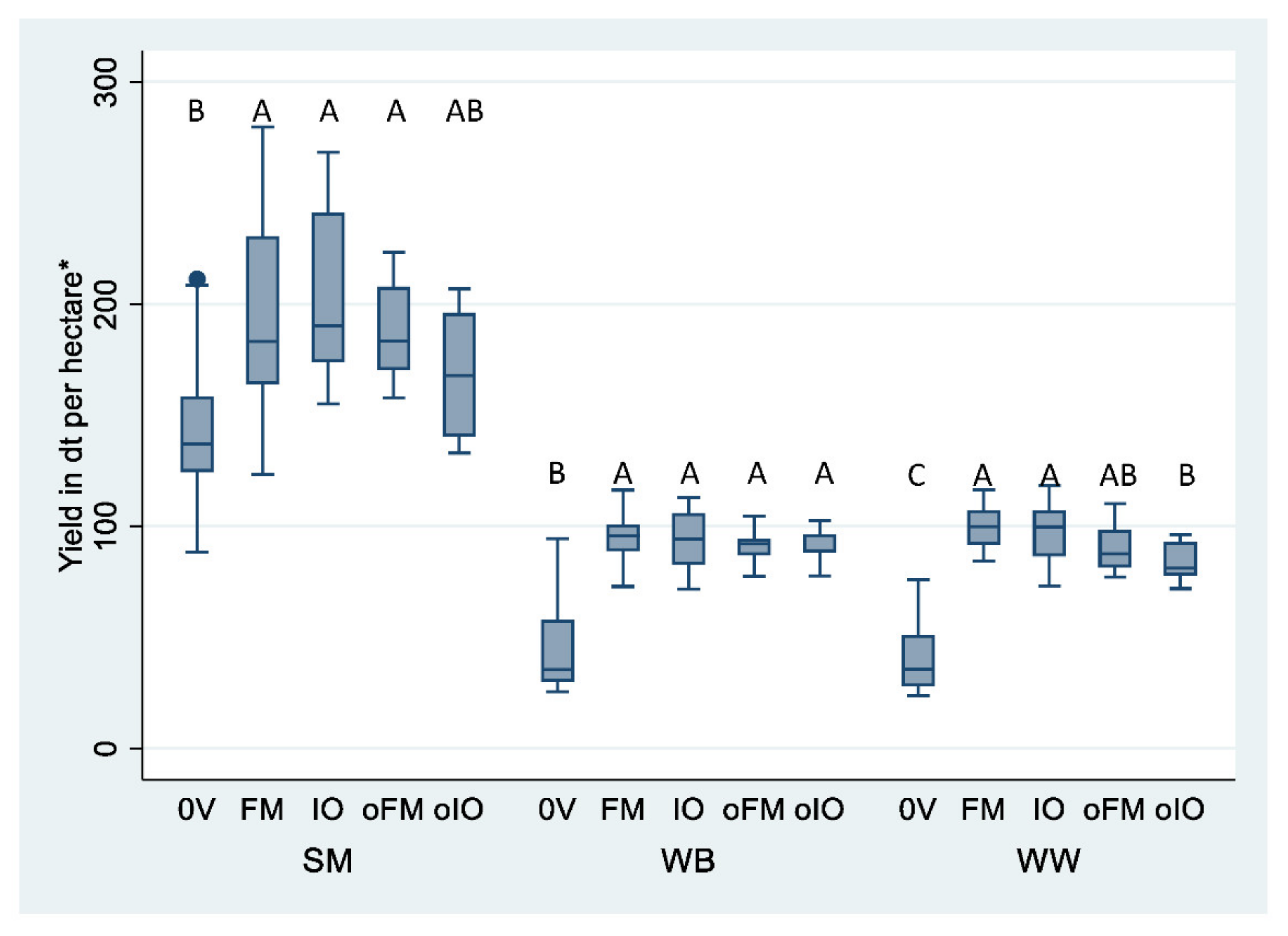
3.2. Analysis of Variance

ANOVA results are presented in

Table 3. Analyses of variance for yield, protein content, and market performance.

Dependent Variable	Y (Yield)		P (Protein)		MP (Revenue)		Y_SM (Yield)		Y_WB (Yield)		Y_WW (Yield)
	F	p	F	p	F	p	F	p	F	p	F	p
Model	32.1	0.000	13.1	0.000	16.5	0.000	3.2	0.000	17.1	0.000	26.9	0.000
f	513.9	0.000	424.8	0.000	798.6	0.000	64.4	0.000	590.7	0.000	655.6	0.000
r	0.5	0.613	1.8	0.233	0.6	0.581	0.5	0.646	1.2	0.343	0.9	0.453
e(F#R)
c	2772.2	0.000	3797.9	0.000	386.8	0.000	---	---	---	---	---	---
c#f	5.4	0.001	41.2	0.000	39.3	0.000	---	---	---	---	---	---
e(R#C#F)
Obs.	297		198		297		99		99		99
Adj R2	0.822		0.640		0.697		0.240		0.697		0.788

Column 1 shows the model structure. Fixed factors are in lower case, random factors are in upper case: f, fertilization; r, replications; and c, culture. Interactions are indicated by #. Dependent variable under investigation is defined by the column headings.

and considered in more detail below.

The influence of dependent variable f (fertilization) was significant in all models (p < 0.001). When factor c (crop) was included in the models, it was also significant (p < 0.001). As expected, variable c also explained a large part of the found variance, since differences in mean yield among SM (180.1 dt ha⁻¹), WB (80.4 dt ha⁻¹), and WW (80.6 dt ha⁻¹) were very high. In the first two models, the interpretation of the primary factors was biased due to a significant interaction term of fertilization and crop. Thus, there were interactions between these two factors that suggested that the fertilization factor was not equally effective in all crops. Closer data analysis (Figure 4) shows that SM responded with lower yield increases to the fertilization factor compared to the two other crops. This finding explains the significant interaction term. Additionally, the adjusted coefficient of determination indicates that the models were able to explain a large part of the found variance. Only the model for SM yield (Y_SM) was an exception, with a coefficient of determination of 0.240. Fertilization had a significant effect, but it is likely that unobserved effects, such as environmental influences, played a much larger role in this model than they did in the other models.

ANOVA confirmed the significance of fertilization in determining yield and differences in yield at different fertilization levels. A pairwise comparison of means (Tukey test) in combination with a box-plot diagram illustrates the yield differences within crops, differentiated by fertilizer level (see Figure 4).

Regardless of crop, there was a significant effect of fertilization compared with in the control (0V). However, for the evaluation of DSS IoFarm, direct comparisons of the variants were necessary. For FM and IO, the location and dispersion parameters in the box-plot diagram indicated that no significant differences were to be expected, which was also statistically proven (

Table 4. Mean values (Ø), standard errors (SE), and Tukey groups (Gr.) for protein content (P), market performance (MP), and crop yields (Y) for five factor levels of fertilization.

		P			MP			Y_SM			Y_WB			Y_WW
	Ø	SE	Gr.	Ø	SE	Gr.	Ø	SE	Gr.	Ø	SE	Gr.	Ø	SE	Gr.
0V	9.17	0.22	B	760.5	32.5	C	142.1	6.85	B	44.7	2.58	B	40.9	2.33	C
FM	12.13	0.23	A	1442.9	32.6	A	195.4	6.85	A	95.3	2.58	A	99.6	2.33	A
IO	11.96	0.24	A	1440.2	32.7	A	203.1	6.85	A	93.8	2.58	A	97.5	2.33	A
oFM	11.11	0.38	A	1338.0	56.2	AB	188.1	11.87	A	91.5	4.47	A	89.5	4.04	AB
oIO	11.03	0.38	A	1256.2	56.2	B	171.3	11.87	AB	91.7	4.47	A	83.7	4.04	B

Means sharing a letter in the group were not significantly different at the 5% level.

). For variants oFM and oIO in which additional organic fertilization was applied, slight negative yield effects were evident compared with those in purely mineral fertilization variants. In all cases, there were no significant differences between the two organomineral fertilized variants. For SM, only variant oIO was not significantly different from the control. For WW, there were significant differences between the oIO variant and the mineral variants, which was not the case for the oFM variant. These observations indicate that there could be slight disadvantages to using IoFarm in the case of organomineral fertilization. For a more detailed assessment of the results, the grouped mean values of the yields, the standard errors (SE), and the classification into Tukey groups are provided in Table 4.

3.3. Effects on Protein Content in Cereals

Overall, protein content plays an important role in determining the market and feed value of cereals, and it is particularly influenced by nitrogen fertilization. Therefore, it is important to measure this quality parameter when comparing fertilizer systems. ANOVA (Table 3) showed that the primary effects that were tested (fertilization, crop, and their interaction) had significant influence on the protein content in cereal grains. A pairwise comparison of means (Tukey test) illustrates the differences in cereal protein content, differentiated by fertilizer level (Table 4, Column P). There were no significant differences in the protein content in the dry matter of all fertilized variants. They only differed significantly from the nonfertilized control. Nevertheless, cereal protein content tended to be somewhat lower in the IoFarm variants. Dilution effects could be excluded in view of the observed yields. Due to the comparable fertilization intensity of the treatments, a possible effect on the protein content is best sought in the dosage and timing of late fertilization.

3.4. Effects of IoFarm Decision Support System on Market Performance

From an economic point of view, it is useful to determine whether fertilization decisions made with the help of IoFarm can achieve comparable market performance to that of fertilization strategies decided by farm managers. This was determined by comparing market performance (calculated according to Equation (5)). For WW, protein content was also used to indicate quality, which determines the market price. A complete overview of the underlying market prices is provided in

Table 5. Overview of postharvest prices in 2016 to 2018 for silage maize (SM), winter barley (WB), and winter wheat (WW).

Crop	Year	2016	2017	2018
SM	EUR (dt DM)−1	8.13	8.00	8.20
WB	EUR dt−1	11.68	12.60	14.36
WW <12% XP	EUR dt−1	12.62	14.16	14.90
WW >12% XP	EUR dt−1	14.01	14.73	15.41
WW >13% XP	EUR dt−1	14.52	15.21	15.97
WW >14% XP	EUR dt−1	15.80	16.74	17.27

XP: Protein content in dry matter.

.

ANOVA indicated that fertilization had significant influence on market performance (Table 3). The market performance of variants FM and IO (Table 4, Column MP) could not be statistically distinguished from each other, indicating that IoFarm did not lead to any difference in market performance in the case of these two variants. However, the market performance of organomineral variant oIO was significantly lower than that of FM and IO, but not significantly different to oFM.

3.5. Effects on Yield Components

Less relevant for the economic evaluation of DSS IoFarm is its influence on the yield components in cereals. From a crop-production perspective, however, important relationships become visible with regard to the yield components. These are presented in

Table 6. Yield components of winter barley and winter wheat.

Variant:	0V	FM	IO	oFM	oIO
Thousand-grain mass (g)
Winter barley
GB	45	46	46
RS	42	45	49
TD	47	49	49	49	49
Winter wheat
GB	55	50	51
RS	47	51	51
TD	53	54	56	55	56
Spikes per square meter (number)
Winter barley
GB	484	721	756
RS	357	609	622
TD	392	732	657	665	611
Winter wheat
GB	372	602	544
RS	466	568	502
TD	309	483	452	470	449
Grains per spike (number)
Winter barley
GB	27	31	29
RS	21	34	29
TD	25	28	31	29	31
Winter wheat
GB	29	34	37
RS	16	37	41
TD	22	36	35	35	34

Variants: 0V = control; FM = farm manager; IO = IoFarm; oFM and oIO additionally treated with organic fertilizer. Sites: GB = Geiselsberg; RS = Roggenstein; TD = Triesdorf.

and thus enable a more detailed agronomic interpretation of the results.

Apart from the control, the differences in thousand-grain weight were moderate. The main differences between the FM and IO or oFM and oIO variants relate to the number of spikes per square meter and the grains per spike. On the basis of this observation, it can be concluded that the timing or synchronization between nitrogen fertilization and nitrogen uptake was different among test varieties. A model-internal consideration of variety characteristics in IoFarm could lead to significant improvements, and possibly contribute to the stabilization of the yield reliability of IoFarm.

4. Discussion

The main purpose of this study was to compare the agronomic performance of the IoFarm DSS with a standard farm-fertilization strategy in a field trial. From this, it was deduced whether fertilization strategies calculated by IoFarm or by similar DSSs could be expected to have agronomic impact. Results from Table 4 (compared Tukey groups) showed that there were no significant effects of yield, protein content, and market performance within comparable variants, with and without organic fertilization. Hence, IoFarm does not impair agronomic outcomes. The literature does not provide any studies on the agronomic effects of DSSs with similar objectives. DSSs with similar objectives are considered to be that by Pagán et al. [17], by Bueno-Delgado et al. [16], Smart Fertilizer Management [15], and by Villalobos et al. [33]. They also have a clear focus on the least-cost combination of fertilizers, and consider at least nutrients nitrogen, phosphorus, and potash in parallel. In contrast, numerous other studies mainly deal with the optimal intensity of fertilization and provide valuable knowledge in this area: For example, Wu and Ma [34], who state in their review that integrated nutrient management is of great importance for global crop productivity, or Rajsic and Weersink [28], and Mandrini et al. [14], focusing on economically optimal nitrogen supply. More broadly, some field-tested DSSs that simulate or recommend the use of inputs in crop production were studied and found to be useful in enabling agronomic performance [10,11,12,13]. These studies are based on crop-growth models, or apply ex ante versus ex post analysis. However, an estimation of potential agronomic effects caused by a primarily cost-optimized fertilization strategy (as, e.g., in IoFarm) is not possible with the help of these studies. This study fills that gap and shows that a primarily cost-optimized fertilization strategy can keep up the pace with a standard farm-fertilization strategy from an agronomic perspective.

Before further discussion of the results, some limitations should be noted: due to the relatively high variance of the dependent variable within the control variant, the requirements of ANOVA for homoscedasticity were not met in some groups. Efforts to reduce variance by different transformations were unfortunately not successful. If included in the respective model, interactions of the main factors of f fertilization and c crop were always significant. Strictly speaking, both observations led to an invalid interpretation of ANOVA. The problem of partial heteroscedasticity can be avoided by excluding the control variant from data analysis. However, our focus was on the comparison of the factor levels of fertilization. The Tukey test can be reliably used under these conditions, which is why we decided not to exclude the control variant. For comparison purposes, all group means were checked in parallel with an unadjusted least-significant-difference t-test. Even with this more liberal test, no significant differences were found between comparable variants FM and IO or oFM and oIO.

Predictably, the purely mineral fertilization variants (FM and IO) and the organomineral variants (oFM and oIO) only slightly differed from each other on the basis of their group mean values. Therefore, care was taken in the experimental design to test them under as many environmental conditions (year and location) as possible to obtain enough observations for comparison. The relative standard error indicated, among other things, whether the number of observations were sufficient to clarify the experimental question. In the case of the mineral-fertilized variants, the relative standard error of the yield across all crops was 2.3% to 3.5%. This allowed for a suitable estimation of the significance levels, which again confirmed that no yield effects were expected from using IoFarm instead of standard farm-manager decisions. For organomineral variants, the range of the relative standard error was significantly higher, at 4.5% to 6.9%. Therefore, additional observations are necessary to make a more robust estimation of the significance levels for these variants. This was not possible in the field trial because the necessary plot technology for digestate application was only available in TD. Comparing variants oFM and oIO was also affected by weather and possible fluctuations in the nutrient content in the used digestate: for the fictitious 150 ha farm, 4000 m³ of digestate was available per year, which could be allocated to the crops almost freely in terms of quantity and timing. Thus, it was not possible to guarantee homogeneous weather conditions and homogeneous nutrient content in the digestate between the two variants, which inevitably led to unobserved influences on the nutrient supply. In sum, the comparison of the organomineral variants was significantly weakened. However, findings tend to indicate that farm managers were able to better integrate the digestate into their fertilization planning than in the IoFarm model. Therefore, it might make sense to leave the planning of organic fertilization to the farmer, and to consider this as an external specification in IoFarm, so that operational conditions, such as trafficability of the fields or storage capacities, can also be taken into account. Alternatively, it would be conceivable to adopt such restrictions in IoFarm and redefine the effectiveness of organic fertilizers within the model.

Market performance must be considered to evaluate the economic performance of IoFarm. However, volatile prices add another random factor: changes in price relations influence the contrast between group means, and could also influence whether there are significant differences between groups. It is also possible that farms use the entire grain yield for feed purposes and do not receive the market value, making it necessary to include a substitution value. In this case, the protein content of WB would also affect the substitution value. Analysis of yield, protein content, and market performance led to a largely consistent trend in differences between treatment groups. Therefore, despite the mentioned limitations, it could be assumed that moderate price or value changes did not have a significant influence on the assessment of market performance.

The financial-savings potential of using IoFarm was investigated in an independent experiment [1]. Results showed that the IoFarm DSS leads to an average cost saving of 66 EUR ha⁻¹. This savings potential is mainly based on the least-cost combination of fertilizers, at largely identical nutrient inputs. In comparison, according to [35], the savings potential of sensor-based fertilizer systems ranges from 33 to 92 EUR ha⁻¹, whereas manufacturing companies assume savings of 20 to 30 EUR ha⁻¹. At least comparable results were obtained using IoFarm without additional technical equipment. As no significant differences were found in yield, protein content, and market performance for the mineral variants, the mentioned cost advantage could be fully attributed to using the IoFarm DSS. In the case of organomineral variants, the reliability of the results was less robust. In a direct comparison, variants oFM and oIO were not found to be significantly different. However, in contrast to oFM, oIO was somewhat behind the mineral-fertilized variants in terms of production. Therefore, if organic fertilizers are used, the oFM variant tends to have an advantage from an agronomic point of view. The actual extent of this difference and whether it is compensated for by the cost optimization of the fertilization strategy requires further investigation.

5. Conclusions

Our findings and the previous literature indicate that carefully developed DSSs are able to provide superior solutions in complex situations. When optimizing a fertilization strategy, IoFarm considers a large amount of information and restrictions, which is not possible for decision makers to process. Through this computation ability, IoFarm can save fertilizer costs without having to accept a reduction in yield and quality. Therefore, a cost-optimized fertilization strategy is not fundamentally in conflict with other agronomic objectives. The benefits for farmers and their advisors are evident: lower costs with the same levels of market performance. Since the search for a least-cost fertilization strategy is of global importance, the results of this study are also of international interest. However, by adapting the objective function, further objectives could also be achieved using IoFarm: instead of a least-cost fertilization strategy, minimizing the CO₂ footprint associated with fertilization could also be optimized. Therefore, CO₂-efficient fertilization strategies could be developed, which is important in the context of climate change, both socially and internationally. However, further research is needed to determine CO₂ emissions caused by individual fertilizers. Currently, it is necessary to expand the range of available crops in the IoFarm DDS to enable broad applicability for farmers and consultants. The final goal is to enable farmers to directly use IoFarm. For this purpose, the data exchange must be performed via an online platform. For a high level of user friendliness, it is important that digitally available farm data can be imported. The calculation of an optimal fertilizer strategy is then carried out via external servers with high computing capacity. The result is stored in the online platform and made digitally available to farmers in the form of a fertilization strategy.

References

1. Tröster, M.F.; Sauer, J. IoFarm: A novel decision support system to reduce fertilizer expenditures at the farm level. Comput. Electron. Agric. under review.
2. Tian, C.; Zhou, X.; Liu, Q.; Peng, J.; Zhang, Z.; Song, H.; Ding, Z.; Zhran, M.A.; Eissa, M.A.; Kheir, A.M.S.; et al. Increasing yield, quality and profitability of winter oilseed rape (Brassica napus) under combinations of nutrient levels in fertiliser and planting density. Crop Pasture Sci. 2020, 71, 1010. [Google Scholar] [CrossRef]
3. Ransom, C.J.; Kitchen, N.R.; Camberato, J.J.; Carter, P.R.; Ferguson, R.B.; Fernández, F.G.; Franzen, D.W.; Laboski, C.A.M.; Nafziger, E.D.; Sawyer, J.E.; et al. Corn nitrogen rate recommendation tools’ performance across eight US midwest corn belt states. Agron. J. 2020, 112, 470–492. [Google Scholar] [CrossRef] [Green Version]
4. Hlisnikovský, L.; Vach, M.; Abrhám, Z.; Mensik, L.; Kunzová, E. The effect of mineral fertilisers and farmyard manure on grain and straw yield, quality and economical parameters of winter wheat. Plant Soil Environ. 2020, 66, 249–256. [Google Scholar] [CrossRef]
5. Mi, W.; Gao, Q.; Guo, X.; Zhao, H.; Xie, B.; Wu, L. Evaluation of Agronomic and Economic Performance of Controlled and Slow-Release Nitrogen Fertilizers in Two Rice Cropping Systems. Agron. J. 2019, 111, 210–216. [Google Scholar] [CrossRef]
6. Schätzl, R.; Reisenweber, J.; Schägger, M.; Frank, J. LfL Deckungsbeiträge und Kalkulationsdaten. Available online: https://www.stmelf.bayern.de/idb/winterweizen.html (accessed on 14 October 2019).
7. Mariappan, P. Operations Research: An Introduction; Dorling Kindersley: New Delhi, India, 2013; ISBN 9789332517813. [Google Scholar]
8. Scharf, P.C.; Shannon, D.K.; Palm, H.L.; Sudduth, K.A.; Drummond, S.T.; Kitchen, N.R.; Mueller, L.J.; Hubbard, V.C.; Oliveira, L.F. Sensor-Based Nitrogen Applications Out-Performed Producer-Chosen Rates for Corn in On-Farm Demonstrations. Agron. J. 2011, 103, 1683–1691. [Google Scholar] [CrossRef]
9. Jame, Y.W.; Cutforth, H.W. Crop growth models for decision support systems. Can. J. Plant Sci. 1996, 76, 9–19. [Google Scholar] [CrossRef]
10. Araya, A.; Prasad, P.; Gowda, P.H.; Afewerk, A.; Abadi, B.; Foster, A.J. Modeling irrigation and nitrogen management of wheat in northern Ethiopia. Agric. Water Manag. 2019, 216, 264–272. [Google Scholar] [CrossRef]
11. Übelhör, A.; Munz, S.; Graeff-Hönninger, S.; Claupein, W. Evaluation of the CROPGRO model for white cabbage production under temperate European climate conditions. Sci. Hortic. Amst. 2015, 182, 110–118. [Google Scholar] [CrossRef]
12. Chuan, L.; He, P.; Pampolino, M.F.; Johnston, A.M.; Jin, J.; Xu, X.; Zhao, S.; Qiu, S.; Zhou, W. Establishing a scientific basis for fertilizer recommendations for wheat in China: Yield response and agronomic efficiency. Field Crop Res. 2013, 140, 1–8. [Google Scholar] [CrossRef]
13. Sønderskov, M.; Fritzsche, R.; de Mol, F.; Gerowitt, B.; Goltermann, S.; Kierzek, R.; Krawczyk, R.; Bøjer, O.M.; Rydahl, P. DSSHerbicide: Weed control in winter wheat with a decision support system in three South Baltic regions—Field experimental results. Crop Prot. 2015, 76, 15–23. [Google Scholar] [CrossRef]
14. Mandrini, G.; Bullock, D.S.; Martin, N.F. Modeling the economic and environmental effects of corn nitrogen management strategies in Illinois. Field Crop Res. 2021, 261, 108000. [Google Scholar] [CrossRef]
15. Smart Fertilizer Management. Smart Fertilizer; London. Available online: https://www.smart-fertilizer.com/ (accessed on 20 June 2021).
16. Bueno-Delgado, M.V.; Molina-Martínez, J.M.; Correoso-Campillo, R.; Pavón-Mariño, P. Ecofert: An Android application for the optimization of fertilizer cost in fertigation. Comput. Electron. Agric. 2016, 121, 32–42. [Google Scholar] [CrossRef]
17. Pagán, F.J.; Ferrández-Villena, M.; Fernández-Pacheco, D.G.; Rosillo, J.J.; Molina-Martínez, J.M. Optifer: AN application to optimize fertiliser costs in fertigation. Agric. Water Manag. 2015, 151, 19–29. [Google Scholar] [CrossRef]
18. Offenberger, K.; Wendland, M. Düngebedarfsermittlung; Bayerische Landesanstalt für Landwirtschaft, Freising. Available online: https://www.stmelf.bayern.de/npk/app/demo?3 (accessed on 20 June 2021).
19. Kersebaum, K.C. Die Simulation der Stickstoff-Dynamik von Ackerböden. Ph.D. Thesis, University of Hannover, Hannover, Germany, 1989. [Google Scholar]
20. Vanclooster, M.; Viaene, P.; Diels, J.; Christiaens, K. WAVE; Institute for Land and Water Management: Leuven, Belgium, 1996. [Google Scholar]
21. Abrahamsen, P.; Hansen, S. Daisy: An open soil-crop-atmosphere system model. Environ. Modell. Softw. 2000, 15, 313–330. [Google Scholar] [CrossRef]
22. Nendel, C.; Specka, X.; Berg, M. MONICA—The Model for Nitrogen and Carbon in Agro-Ecosystems. Available online: https://www.monica.agrosystems-modles.com (accessed on 20 June 2021).
23. Wendland, M.; Diepolder, M.; Offenberger, K.; Raschbacher, S. Leitfaden für die Düngung von Acker- und Grünland, Freising. 2018. Available online: https://www.lfl.bayern.de/mam/cms07/publikationen/daten/informationen/leitfaden-duengung-acker-gruenland_gelbes-heft_lfl-information.pdf (accessed on 20 October 2019).
24. Waldren, R.; Flowerday, A. Growth Stages and Distribution of Dry Matter, N, P and K in Winter Wheat. Agron. J. 1979, 71, 391–397. [Google Scholar] [CrossRef]
25. Reiner, L.; Dörre, R. Weizen Aktuell, 2nd ed.; DLG-Verlag: Frankfurt am Main, Germany, 1992; ISBN 3769004973. [Google Scholar]
26. Lütke Entrup, N. (Ed.) Lehrbuch des Pflanzenbaues; Verlag Th. Mann: Gelsenkirchen, Germany, 2000; ISBN 378620117X. [Google Scholar]
27. Agrarmeteorologie Bayern. Weather Data in Bavaria. Available online: https://www.wetter-by.de/Internet/global/inetcntr.nsf/dlr_web_full.xsp?src=98OE9BL691&p1=6BH7UJ4826&p3=S313638Z32&p4=YNDMXE6MAN# (accessed on 17 November 2019).
28. Rajsic, P.; Weersink, A. Do farmers waste fertilizer? A comparison of ex post optimal nitrogen rates and ex ante recommendations by model, site and year. Agric.Syst. 2008, 97, 56–67. [Google Scholar] [CrossRef]
29. Tröster, M.F.; Sauer, J. Characteristics of Cost Efficient Fertilization Strategies at Farm Level. manuscript in preperation.
30. StataCorp. Stata Statistical Software; StataCorp LLC.: College Station, TX, USA, 2017. [Google Scholar]
31. Salkind, N.J. Encyclopedia of Research Design; SAGE Publications: Thousand Oaks, CA, USA, 2010; ISBN 9781412961271. [Google Scholar]
32. Directive (EU) 2016/2284 of the European Parliament and of the Council on the Reduction of National Emissions of Certain Atmospheric Pollutants: NEC Directive. Off. J. Eur. Union 2016, L344, 1–31.
33. Villalobos, F.J.; Delgado, A.; López-Bernal, Á.; Quemada, M. FertiliCalc: A Decision Support System for Fertilizer Management. Int. J. Plant Prod. 2020, 14, 299–308. [Google Scholar] [CrossRef]
34. Wu, W.; Ma, B. Integrated nutrient management (INM) for sustaining crop productivity and reducing environmental impact: A review. Sci. Total Environ. 2015, 512–513, 415–427. [Google Scholar] [CrossRef]
35. Evangelou, E.; Stamatiadis, S.; Schepers, J.S.; Glampedakis, A.; Glampedakis, M.; Dercas, N.; Tsadilas, C.; Nikoli, T. Evaluation of sensor-based field-scale spatial application of granular N to maize. Precis. Agric. 2020, 21, 1008–1026. [Google Scholar] [CrossRef]
Figure 1. Workflow of DSS IoFarm: (grey) data input, (orange) execution, (blue) data output.
Agriculture 11 00571 g001
Figure 2. Weather conditions during trial period by location.
Agriculture 11 00571 g002
Figure 3. Similarities and differences in fertilizer strategy: Farm Manager and IoFarm.
Agriculture 11 00571 g003
Figure 4. Location and dispersion measures for different crop yields grouped by level of fertilizer application (n = 297). Levels of fertilization: 0V = no fertilization (n = 3 × 27); FM = farm manager variant (n = 3 × 27), IO = model variant (n = 3 × 27); oFM = FM + organic fertilization (n = 3 × 9); oIO = IO + organic fertilization (n = 3 × 9). Within a crop (SM, WB, and WW), the following applied: means sharing a letter in the group were not significantly different at the 5% level. * For SM, yield refers to dry matter; for WB and WW, yield was corrected to 86% of dry-matter content.
Agriculture 11 00571 g004