Article

Impact of Climate Change on Rice Yield in Malaysia: A Panel Data Analysis

by
Boon Teck Tan
1,
Pei Shan Fam
1,
R. B. Radin Firdaus
2,*,
Mou Leong Tan
3 and
Mahinda Senevi Gunaratne
2
1
School of Mathematical Sciences, Universiti Sains Malaysia, Pulau Pinang 11800, Malaysia
2
School of Social Sciences, Universiti Sains Malaysia, Pulau Pinang 11800, Malaysia
3
Geoinformatic Unit, Geography Section, School of Humanities, Universiti Sains Malaysia, Pulau Pinang 11800, Malaysia
*
Author to whom correspondence should be addressed.
Agriculture 2021, 11(6), 569; https://doi.org/10.3390/agriculture11060569
Submission received: 19 April 2021 / Revised: 17 June 2021 / Accepted: 18 June 2021 / Published: 21 June 2021
(This article belongs to the Section Ecosystem, Environment and Climate Change in Agriculture)

Abstract

:
Climate change is a global problem since many countries worldwide are becoming increasingly vulnerable to natural disasters. Numerous climate models in various studies project a decline in agricultural productivity that will mainly be due to excessive heat in tropical and subtropical regions, especially in Southeast Asia. As a Southeast Asian country, Malaysia is no exception to this problem. Hence, the present study aimed to examine the impact of climate change on rice yields in Malaysia. A panel data approach was adopted using data from 1987 to 2017 on eight granary areas in Peninsular Malaysia. The main objectives were to assess the impact of climate variables (i.e., minimum and maximum temperature and precipitation) on rice yield and the variance of the impact during the main season and off-season. Our regression results indicate that precipitation was not statistically significant in all model specifications for both the main and off-season. While the maximum temperature was found to be negatively associated with yield during the off-season, the minimum temperature showed a positive effect in both cropping seasons. We used the HadGEM3-GC31 N512 resolution model based on the high-emission Shared Socioeconomic Pathways 8.5 scenario (SSPs-8.5) from the High-Resolution Model Intercomparison Project (HighResMIP) of the Coupled Model Intercomparison Project Phase 6 (CMIP6) to project future climate change in 2030 and 2040. The projected results indicate that rice yield would show a more positive trend by 2040 when compared to the previous decade, ranging from −0.02 to 19.85% during the main season and −2.77 to 7.41% during the off-season. Although rice yield is likely to increase in certain areas, other areas are projected to experience negative effects. Hence, adaptation at the farm level remains crucial, specifically during the off-season, since climate change could widen the gaps in rice yields between cropping seasons and among granary areas.

1. Introduction

The global climate has been changing noticeably over recent decades, which is a global phenomenon that is expected to continue. According to the Intergovernmental Panel on Climate Change (IPCC), climate change is defined as changes in the climate that can be identified by changes in the mean or variability of the climate properties and that persists for an extended period, typically decades or longer [1]. Adverse and intense climate events continued during the 2010–2019 period, which was the warmest decade on record globally. Notably, it is projected that the global temperature will increase by 3.2 °C by the year 2100 [2]. Global warming is indisputable since global average daily maximum and minimum temperatures have increased by 1 to 3 °C since 1950, primarily in the Eurasian region [1]. Projections suggest that global mean temperature increases will have adverse impacts such as increased heatwaves, agricultural droughts, floods, and reduced crop yields [3]. A recent study by Firdaus et al. [4] indicated that minimum and maximum temperatures in the main rice granary areas of Peninsular Malaysia have continued to rise rapidly over the past decade, with increases of 0.3 to 0.5 °C and 0.2 to 0.3 °C, respectively.
Since agriculture relies on climate cycles and weather patterns, climate change is expected to affect the productivity of crops, including rice. For instance, a 4% increase in temperature against pre-industrial levels will increase the probability of damaging maize and rice crops due to hot spells by 5 to 50% and 27 to 46%, respectively [3]. Lobell et al. [5] evaluated climate change impacts on 18 different crops in 12 food-insecure regions. These regions covered South Asia, China, Southeast Asia, East Africa, Central Africa, Southern Africa, West Africa, Central America and the Caribbean, the Sahel, West Asia, the Andean region, and Brazil. The results reveal that rice productions in Brazil, Central America, and Southeast Asia are projected to record losses of up to 5% by 2030. Other crops such as wheat in South Asia, the Sahel, Southern Africa, Brazil, and Central Africa, as well as maize in Southern Africa and groundnut in Western Africa, would also likely be affected by such losses. Rosenzweig et al. [6] made an ambitious attempt to assess the impacts of climate change on multiple crops worldwide. Their results indicate that climate change impacts are severe in tropical areas, particularly for annual C3 crops such as rice. In a global assessment of climate change and socioeconomic impacts on agriculture up to 2080 using different models, Fischer et al. [7] found that the critical asymmetric impacts of climatic and socioeconomic factors would increase existing gaps in food production and consumption between developed and developing countries.
For rice, elevated temperatures could reduce grain-filling duration, while extreme temperatures during the flowering phase could reduce the grain or seed volume [8]. In tropical climate countries such as Malaysia, high temperature is a constraint to rice production [4,9,10]. Moreover, variability in the amount and distribution of precipitation (which could lead to drought and/or flooding) is another crucial factor that could affect the yield of rain-fed rice, especially in low altitude regions [11,12,13,14] such as those located in Malaysia [4,9,10]. For instance, a study conducted using the DSSAT crop simulation model found that rice yield in Malaysia will decrease by 12% in the main season and 31.3% in the off-season until 2030 as temperatures increase and precipitation patterns change [15]. A study conducted in Northwest Selangor, Malaysia, identified the negative impacts of temperature and precipitation variants on rice production while emphasizing the location-specific impacts of climate change [16]. In a global scale study on impacts of climate change at different temperature levels on crop yields, Arnell et al. [3] found that dry spell may have damaging impacts on rice and maize yield yet projected regional variations.
Several studies projected that increased atmospheric carbon dioxide (CO2) concentration along with temperature, precipitation, soil conditions, and solar radiation would have mixed impacts on rice yields. Under a high CO2 emission scenario (CO2 at 900 ppm), rice and soybeans in the U.S. will have a 135% increase in yield in 2100 due to the CO2 fertilization effect [17]. However, impacts of increased CO2 (850 ppmv) and temperature (38 °C) on the M206 rice variety in California, U.S., caused a 16% reduction in yield [18]. While in Southwestern China, increased temperature and CO2 (at 700 ppm) will result in decreased rice yield up to 10.5% by 2050 and 47.9% by 2080 [19]. Ujiie et al. [20] found that elevated atmospheric CO2 reduces nutritional elements (zinc, protein, and iron) in C3 type grain crops and legumes, possibly due to lower absorption or translocation of such nutrients under CO2 concentration. Thus, they proposed to move from C3 to C4 crops and genetic modifications in C3 grain crops. More importantly, changes in micronutrients, minerals, protein, and vitamins in different 18 rice varieties in Asia would have negative consequences on rice-consuming countries. These risks may range from health impacts to lower gross domestic product, thus impact on about 600 million people [21]. As per Ujiie et al. [20], elevated CO2 may affect nutritional values in grain crops, feed crops, and leaf vegetables (such as nitrogen, zinc, calcium, magnesium, and sulfur), thus causing a greater threat to human health and nutrition. Therefore, it is obvious that changing climate and agronomic conditions, as well as increased CO2 in the atmosphere, bring both positive and negative impacts.
In general, three main approaches have been widely used to analyze the impacts of climate change on agriculture—one of which is panel data analysis [22]. In panel data analysis, omitted variables can be overcome by including regional dummies in the model. This method has been applied in many studies, such as those of Arnell et al. [3], Welch et al. [23], Sarker et al. [24], and Mahrous [25]. The panel model most commonly applies two types of effect models, namely fixed- and random-effects models. Most of the aforementioned studies used the fixed-effects model because district-specific characteristics can be included in this model. Moreover, the random-effects model does not require a correlation between unobserved time-invariant characteristics and the explanatory variable, while the fixed-effects model relaxes this assumption [26].
Malaysia is located in Southeast Asia, lying just north of the equator. Malaysia is categorized as equatorial, hot, and humid throughout the year, with average daily temperatures ranging from 21 to 32 °C throughout the year [27]. The average annual rainfall of Peninsular Malaysia is approximately 2500 mm [28]. In major granary areas, rice is cultivated twice per year during the off-season (March to July) and the main season (August to February). The main season has high air humidity due to the heavy rainfall brought on by the northeast monsoon, while the off-season has low air humidity with less rainfall [9]. Rice production in Malaysia mainly comes from these granary areas, which produced approximately 74% of the total national production in 2016. However, the average yield per hectare varies among different granary areas due to location-specific factors such as environmental conditions, cultivation areas, and farming practices [29].
Several studies have found that climate variables have a significant impact on agriculture yield [30]. Climate parameters such as increased temperature, high or low precipitation as well as extreme weather events adversely affect crop productions, thus challenging food security [4]. Studies projected that increased atmospheric CO2 concentration would have a mixture of positive and negative effects on rice production, consumption, distribution as well as national development [17,18,19,20]. Extreme weather events due to climate change alter the food production, consumption, trade, and distribution patterns, thus challenging poverty eradication, food security, and sustainable development [4,7]. Moreover, climate change has negative adverse impacts on agriculture, especially at low latitudes and tropical areas [6,30]. Since a continuous temperature rise is anticipated [31], assessing the impacts of climate change on Malaysian rice yield is crucial. Notably, a limited number of studies in Malaysia have used panel data analysis to assess the impact of climate change. Therefore, the present study specifically aimed to analyze the impact of climate variables on rice yield in Peninsular Malaysia during the main and off-season.

2. Materials and Methods

2.1. Data

A panel data set was used for the present study. In general, panel data analyses use statistical (i.e., regression) techniques to estimate the effect of climate parameters on crop yields by estimating a production function. In contrast, the empirical estimation of these functions is based on panel data, which includes observations of a cross-section of individual units (i.e., granary areas) over time [22]. Data from granary areas (i.e., yield and cultivated area) were obtained from the Ministry of Agriculture (MOA), while climate data were provided by the Malaysian Meteorological Department (MMD). Granary data were seasonal, while daily meteorological records (i.e., minimum temperature, maximum temperature, and precipitation) were taken from eight weather stations in Peninsular Malaysia (see Table 1).
The empirical analysis was based on panel data involving eight granary areas in Peninsular Malaysia from 1987 to 2017. Figure 1 illustrates the locations of these granary areas and their closest weather stations (as indicated in Table 1). We used the same weather station data for the S.P. and B.L.S. granary areas, which was collected from the Hospital Teluk Intan Station. Moreover, KADA and K.S. used data from the Kota Bharu station. Both KADA and K.S. are located in Kelantan, which can be best represented by the Kota Bharu station. For the S.P. and B.L.S. granary areas, there is only one central station between these areas: the Hospital Teluk Intan Station.
Wetland rice varieties in the main granary areas are cultivated during both cropping seasons (i.e., the main season and off-season). Hence, we formed the data into a seasonal data set. In every cropping calendar, the off-season typically runs from March to July, while the main season begins in August of the same year and ends in February of the following year [9]. The rice yield data provided for each granary area are measured in kilograms per hectare (kg/ha).
Regarding the climate data, three weather variables were considered: precipitation (mm), minimum temperature (°C), and maximum temperature (°C). Since the data provided by the MMD were daily observations, the cumulative amount of precipitation was calculated according to the respective season (the main season runs from March to July while the off-season is from August to February). For instance, daily precipitation values from 1st March until 31st July in 1987 were summed to estimate the total precipitation for the off-season in 1987. Regarding minimum temperature data, the daily temperatures during each season were averaged to determine the average seasonal temperature. The same method was also applied to determine the maximum temperature. Hence, all climate data in this study were aligned based on the rice cropping seasons. Table 2 summarizes the variables used in this study.

2.2. Model Specification

The least-squares dummy variable (LSDV) model was applied in this study. The LSDV model allows for heterogeneity among the cross-section by allowing each entity to have an intercept value. The model is defined as:
y it =   α 0 + i = 1 N 1 α i D i + k = 1 K β k x k , it + ε it   for   i = 1 , N ,   t = 1 , , T ,
where N is the number of cross-sections, T is the period, K is the number of independent variables, and y it and x k , it are the dependent and independent observations, respectively, for the ith individual and tth period. Moreover, α i and β k are parameters of interest that measure the impact of the dependent variable, while D i is the dummy variable (value equals 1 when the observation relates to granary i, and 0 otherwise) and ε it the error term.
In this study, we used a fixed-effects model (FEM). For the FEM, we assumed that the regressors’ slope coefficients did not vary across granary areas or over time. This is also known as a time-invariant model, which implies that although the intercept may differ across granary areas, each granary’s intercept does not vary over time.
The fixed- and random-effects models are commonly used in panel models. In this study, the FEM was chosen for few reasons. First, the FEM allows for the specific characteristics of granary areas to be included. One advantage of the fixed-effects over the random-effects model is that the FEM allows for the correlation between regressors and time-invariant distinctiveness. In contrast, the random-effects model assumes no correlation between unobserved time-invariant characteristics and explanatory variables. This decision is also supported by recent studies [32,33].
In this study, we developed four estimation models. Our analysis applied a panel fixed-effect approach that involved eight granary areas over a 31-year period (1987 to 2017). We included four independent variables (i.e., size of cultivation area, precipitation, minimum temperature, and maximum temperature) to analyze the impact of these variables on rice yield. Precipitation and temperature are known as the primary determinants of crop growth and yield. Hence, Model 1 is defined as follows:
lnYield it =   α 0 + i = 1 7 α i D i + β 1 Land it +   β 2 P it +   β 3 Tmin it +   β 4 Tmax it     +   ε it
Model 1 (Equation (2)) is a production function in linear form. This equation examines the linear effect of each explanatory variable on the dependent variable. Model 2 is computed as follows:
lnYield it =   α 0 + i = 1 7 α i D i + β 1 Land it +   β 2 P it +   β 3 Tmin it +   β 4 Tmax it     + β 5 Land it 2 +   β 6 P it 2 +   β 7 Tmin it 2 +   β 8 Tmax it   2   + β 9 P it Tmin it + β 10 P it Tmax it + β 11 Tmin it Tmax it +   ε it
For Model 2 (Equation (3)), the quadratic terms for independent variables were included in the specification to account for the non-linear effect of independent variables on rice yield. An interaction term between the independent variables was included to determine the potential effect of one independent variable (specifically the climatic variables) given the effect of another independent variable. The dependent variable of rice yield was a natural logarithm transformed for both models to reduce the data variability and improve the variable’s distribution. Since only the dependent variable was natural logarithm transformed, the model estimated semi-elasticities. Therefore, interpreting the impact of a one-unit increase in the independent variable (assuming other independent variables remain constant) represents a certain percentage change in yield.

2.3. Diagnostic Tests

Before a model is regressed for prediction, a series of diagnostic tests are required to ensure that the error structure of the model fulfills the assumptions. In this study, three key assumptions need to be satisfied: (1) errors must be homoscedastic; (2) errors must be cross-sectionally independent; (3) autocorrelation is not present. The Breusch-Pagan test was applied to test for the presence of heteroscedasticity. It tests the null hypothesis that the error variances are all equal versus the alternative hypothesis that the error variances are unequal. A test suggested by Wooldridge was performed to assess the presence of autocorrelation [34,35]. The null hypothesis of this test states that there is no first-order autocorrelation, while the alternative hypothesis states otherwise. Lastly, Pesaran’s cross-sectional dependence (CD) test was used to test for the presence of CD under the null hypothesis of CD [36].
We also conducted a unit root test to confirm that our time series data were stationary. If a time series of panel data contains a unit root (non-stationary), it implies that there is a systematic pattern that is unpredictable. The existence of a unit root or regressing non-stationary data will produce a spurious regression. Usually, a regression is spurious if trending variables over time are regressed, which likely indicates a non-existing relationship.
Traditional unit root tests work only with one time series at a time. In this study, the first-generation unit root test assumes no CD (i.e., the Fisher-type test was performed as proposed by Maddala and Wu [37] using the augmented Dickey-Fuller (ADF) test). Additionally, we performed the second generation that allows CD (i.e., the Pesaran unit root test [38]).

2.4. Climate Change Scenarios

The HadGEM3-GC31 N512 high-resolution model (1024 × 768, Had-HM) based on the high-emission Shared Socioeconomic Pathways 8.5 scenario (SSPs-8.5) from the High-Resolution Model Intercomparison Project (HighResMIP) of the Coupled Model Intercomparison Project Phase 6 (CMIP6) [39] was used to extract future climate projections over the eight rice granary areas. The high-resolution HadGEM3-GC31 model was selected due to its greater capability in capturing mean and extreme observed precipitation over Peninsular Malaysia compared to the coarse resolution version [40].
Since original climate models even contain biases in high-resolution versions, a bias correction scheme should be implemented before applying them to regional- or local-scale studies. The quantile mapping approach adopted by Tan et al. [41] to bias correct the CMIP6 HighResMIP models in the Kelantan River Basin, Malaysia, was used in this study. We found that the quantile mapping approach can effectively correct the occurrence period of peak monthly precipitation in December and precipitation amount for all months. The bias-corrected Had-HM model was then used to extract annual precipitation and maximum and minimum temperatures for the historical period (1985 to 2004) and the future periods of 2015–2034 (2030) and 2025–2044 (2040). Precipitation and temperature projections over the eight granary areas are summarised in Table 3.
Both minimum and maximum temperatures are projected to increase significantly across all granary areas. Regarding precipitation, the changes were heterogeneous across the granary areas. MADA, P.P. and K.S.M. are expected to experience a decline in precipitation, while precipitation in the remaining areas is expected to increase by 2030. However, precipitation for MADA is likely to increase by 2040, while P.P. and K.S.M. will remain negative compared to the historical mean.
The maximum and minimum temperature time series are depicted in Figure 2. The time series results showed that the mean annual maximum and minimum temperatures of the granary areas will increase continuously during the 2015–2045 period. The regression line showed a significant increasing trend in mean annual maximum and minimum temperatures (Figure 2a,b). While a time series analysis for precipitation was also performed, the regression line showed a marginally positive trend that was insignificant (Figure 2c).

3. Results and Discussion

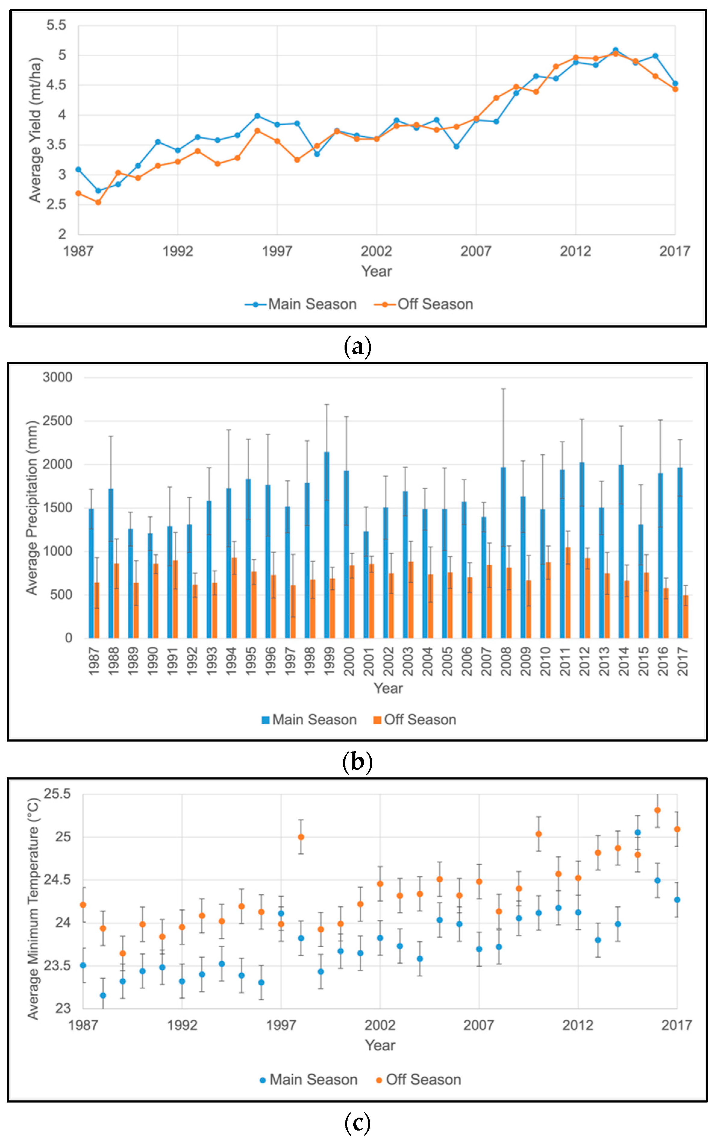
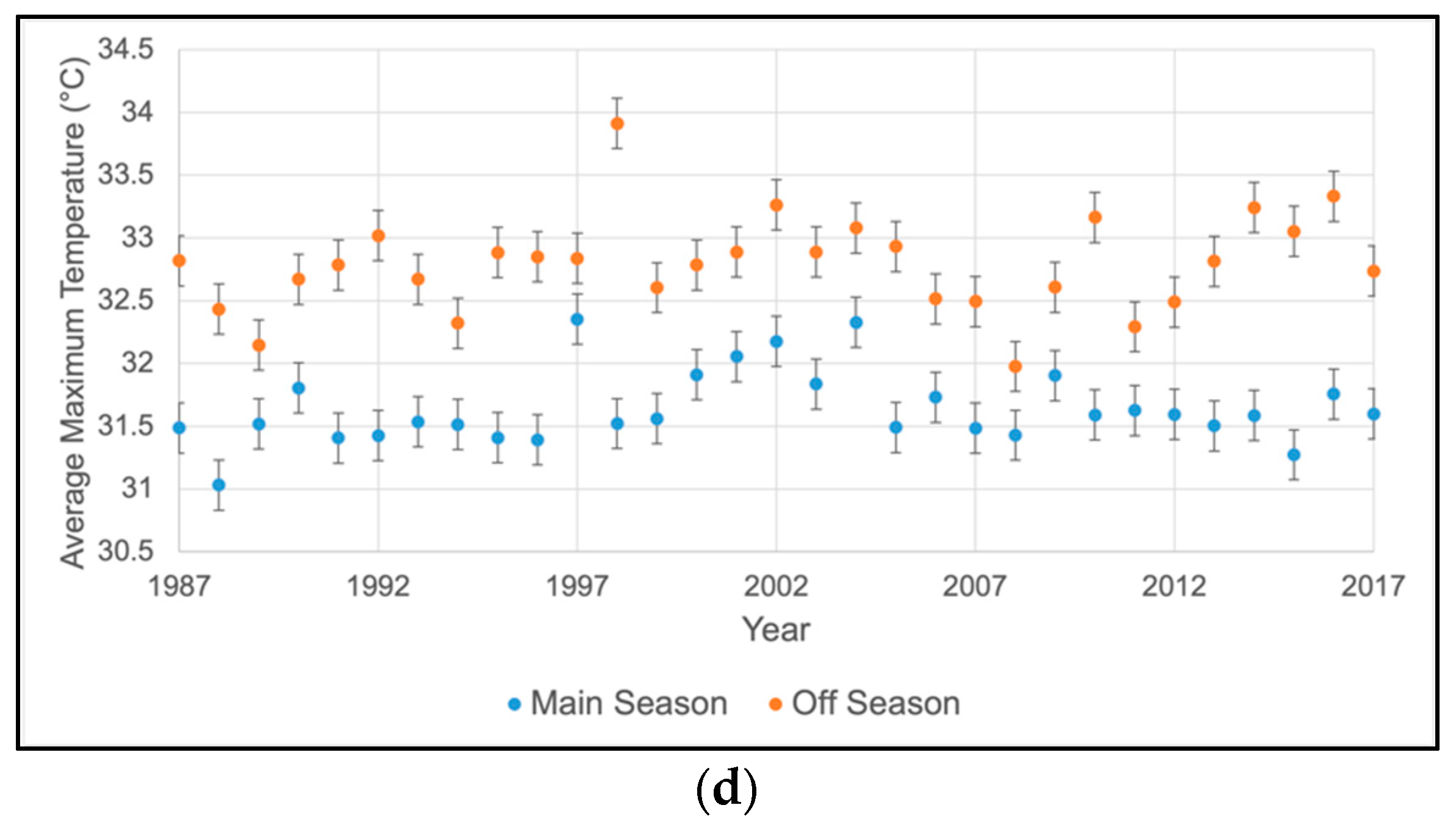
3.1. Descriptive Statistics

Table 4 presents the descriptive statistics of the eight granary areas. In general, B.L.S. had the highest mean annual rice yield (4859.72 kg/ha), while K.S. had the lowest rice yield (2941.07 kg/ha) and granary area (6455.1 ha). Moreover, MADA had the largest cultivation area (192,180.3 ha) with the second-highest mean annual rice yield (4358.78 kg/ha) among the eight areas. Regarding climate variables, KETARA had the highest total precipitation (2680.55 mm), while MADA had the lowest (2046.7 mm). Furthermore, there was not much difference in temperature among the eight granary areas since these areas are located within a relatively small region (i.e., Peninsular Malaysia). Since S.P. and B.L.S. used the same meteorological station, both of these regions had the lowest mean minimum temperature (23.7 °C) despite having the highest mean maximum temperature (33.12 °C).
In addition to comparing regions, analyzing seasonal differences is also essential. Figure 3a–d illustrates the differences in rice yield and climatic variable fluctuation between the main season and off-season over a 31-year period.
These figures strongly support the fact that granary areas in Peninsular Malaysia are usually hotter during the main season when compared to the off-season. Figure 3b shows that there was heavier precipitation during the main season than in the off-season. Furthermore, temperatures (minimum and maximum) during the main season were generally lower than in the off-season (see Figure 3c,d). On the other hand, the average rice yield per hectare (Figure 3a) during the main season was higher than that of the off-season. These results may indicate that precipitation had a positive impact on rice yield, while temperature had a negative impact. Further analyses were conducted to confirm the hypothesis (see Section 3.4).

3.2. Diagnostic Tests

A series of diagnostic tests were conducted before the panel model estimation. To avoid the possible spurious correlation between variables, unit root tests (i.e., Fisher-ADF and Pesaran’s CD test) were conducted. Table 5 exhibits the results of the two tests with and without trends. The values shown in Table 5 include the test statistics and their p-values (in parenthesis). All of the variables assessed were statistically significant in tests with and without trends. Most of the variables were substantially significant at the 1% significance level. This implies that the null hypotheses stating that all panels contain a unit root can be rejected. Therefore, the variables were stationary, and no differencing is required. Hence, estimation of the variables using the model was carried out at the level. As previously mentioned, we developed two models to represent the main season and off-season, respectively. The main season and off-season models’ diagnostic results are shown in Table 5 and were initially estimated using the ordinary least squares (OLS) method.
The Breusch-Pagan test was used to assess the presence of heteroscedasticity. As shown in Table 6, only the main season model had a p-value of 0.406, which was not statistically significant and indicated that the null hypothesis of homoscedasticity could not be rejected despite heteroscedasticity being discovered in the other models. On the other hand, the Wooldridge test was applied to identify the presence of a first-order autocorrelation. In Table 6, all models were statistically significant. Consequently, the null hypothesis of no presence of autocorrelation was rejected.
To assess cross-sectional dependence, we performed Pesaran’s CD test [42]. Since all the p-values were less than 0.001, there was substantial evidence to reject the null hypothesis of cross-sectional independence. Thus, all models were correlated across panel groups, respectively.
Based on the three tests conducted on the four models, all models did not generally fulfill the error assumptions. Thus, using the OLS method to estimate the models would lead to bias problems. Therefore, Equation (1) could not be estimated using the OLS method since its assumptions were violated. Instead, we used a panel-corrected standard error (PCSE) approach while considering the violation of assumptions such as heteroscedasticity, serial correlation, and CD found in the diagnostic tests [43,44]. The PCSE approach retains the OLS parameter estimates but corrects the value of standard errors for parameters estimated by the OLS method.

3.3. Model Estimation

Linear regression with PCSEs for the four models (Model 1–Main and Off-Season and Model 2-Main and Off-Season) is shown in Table 7. All models were significant based on the test statistic (p-values were all less than 0.01). Regarding climate variables, the coefficient of precipitation in linear and quadratic forms was negative but not significant. However, the interaction term between precipitation and minimum temperature was positive and significant, indicating a cumulative impact of these two rice yield variables. Regarding minimum temperature, there was no significant coefficient for the variables in linear and quadratic forms.
Model 2 consists of variables in the linear form and includes the quadratic and interaction terms. Even though the adjusted R2 value for Model 1 is 0.9189, which was higher than for Model 2 (0.9078), the difference was relatively slight. However, there were significant interaction and quadratic terms in Model 2 that must be modeled. Based on the estimated parameters, a few dummy variables showed a significant effect on rice yield, which indicates that the variables successfully captured the heterogeneity across individuals. Moreover, cultivation area (land) was significant in the linear form and positively related to rice yield.
The estimation of Model 2 (off-season) also used PCSEs. As per the main season estimation, the quadratic term elucidates the non-linear relationship between climate variables and yield, while the interaction variables explain the cumulative impact. There were few dummy variables with p-values less than 0.05, indicating an apparent heterogeneity across the granary areas. Moreover, the area of cultivation had a negative coefficient in the linear form. However, the quadratic form was positively significant, indicating a convex relationship with rice yield.
Regarding climate variables, the coefficients of precipitation in linear and quadratic forms were negative but not significant. However, the interaction term between precipitation and minimum temperature was significant, indicating a negative joint impact of these two variables on rice yield. Consequently, precipitation affects rice yield. Similar to precipitation, there were no significant coefficients for variables in linear and quadratic forms for minimum temperature. However, as previously mentioned, there was a significant positive coefficient of the interaction term between precipitation and minimum temperature.
Unlike the main season, precipitation during the off-season has no significant effect on rice yield (even when interacted with other variables). This implies that the amount of precipitation did not affect rice yield during the off-season. Notably, this could be due to the effect of irrigation systems, which was not measured in the model. The irrigation systems in the main granary areas are considered effective, particularly during the off-season period [45]. Regarding minimum temperature, the quadratic term’s coefficient was positive and significant, showing a convex relationship similar to that observed by Gupta et al. [11]. Moreover, there was a negative joint impact of minimum and maximum temperature. There were few dummy variables with p-values less than 0.05, indicating a sturdy heterogeneity across the granary areas. Moreover, the area of the cultivation had a positive coefficient in the linear form. However, the quadratic form was positively significant, indicating a convex relationship with rice yield.
Note, however, the model did not include the effects of carbon dioxide (CO2) fertilization. CO2 fertilization due to an increase in the concentration of atmospheric greenhouse gases is expected to counterbalance the negative effects of climate change and stimulate plant growth [46,47], particularly in the temperate climate zone [48]. In this zone, C3 crops with a lower photosynthetic efficiency rate, such as rice and wheat, will benefit from the increase in atmospheric CO2 [49]. In contrast, C4 crops with a higher rate of photosynthetic efficiencies, such as corn and millet, are projected to experience limited response [50]. If the CO2 concentration is elevated to 550 ppm (parts per million) under normal conditions, C3 and C4 crop yields are projected to increase by approximately 10 to 25% and 0 to 10%, respectively [51]. This is because the increase in CO2 concentration limits the water loss through leaf stomas (the pores on the surface of plants) that goes through transpiration [52].
Crop productivity is affected by counteracting factors (e.g., temperature, precipitation), and increased atmospheric CO2 also leads to increase crop yield. Although elevated CO2 increases the yields of C3 crops by 10 to 30%, crop responses, however, depend on agronomic conditions, types of species, availability of water and nutrients (see Toreti et al. [53] for a recent review). A free-air CO2 enrichment (FACE) experiment in Tsukuba, Japan, using eight rice cultivars demonstrated a wider range of rice yield (3 to 36%) increase due to elevated CO2 [54]. A study by Kimball [55] found that elevated CO2 (353 to 550 ppm) coupled with sufficient nutrients and water result in increased grain yields in C3 crops such as rice, on average about 19%. However, the effects on C3 crop productivity could be minimal when nutrients such as nitrogen are limited [55,56]. Another recent study using indica, japonica, and hybrid rice cultivars has indicated an increased yield of 13.5% for japonica, 22.6% for indica, and 32.8% for hybrid cultivars with an elevated CO2 of about 200 μmol mol−1 above ambient [57]. While studies in the large-scale field environment using FACE show that elevated CO2 strongly affects rice yield [54,55,56,57], our regression results, however, are mainly restricted to the domain of the data. Thus, we caution that our results could be affected by the exclusion of the beneficial effects of elevated CO2.

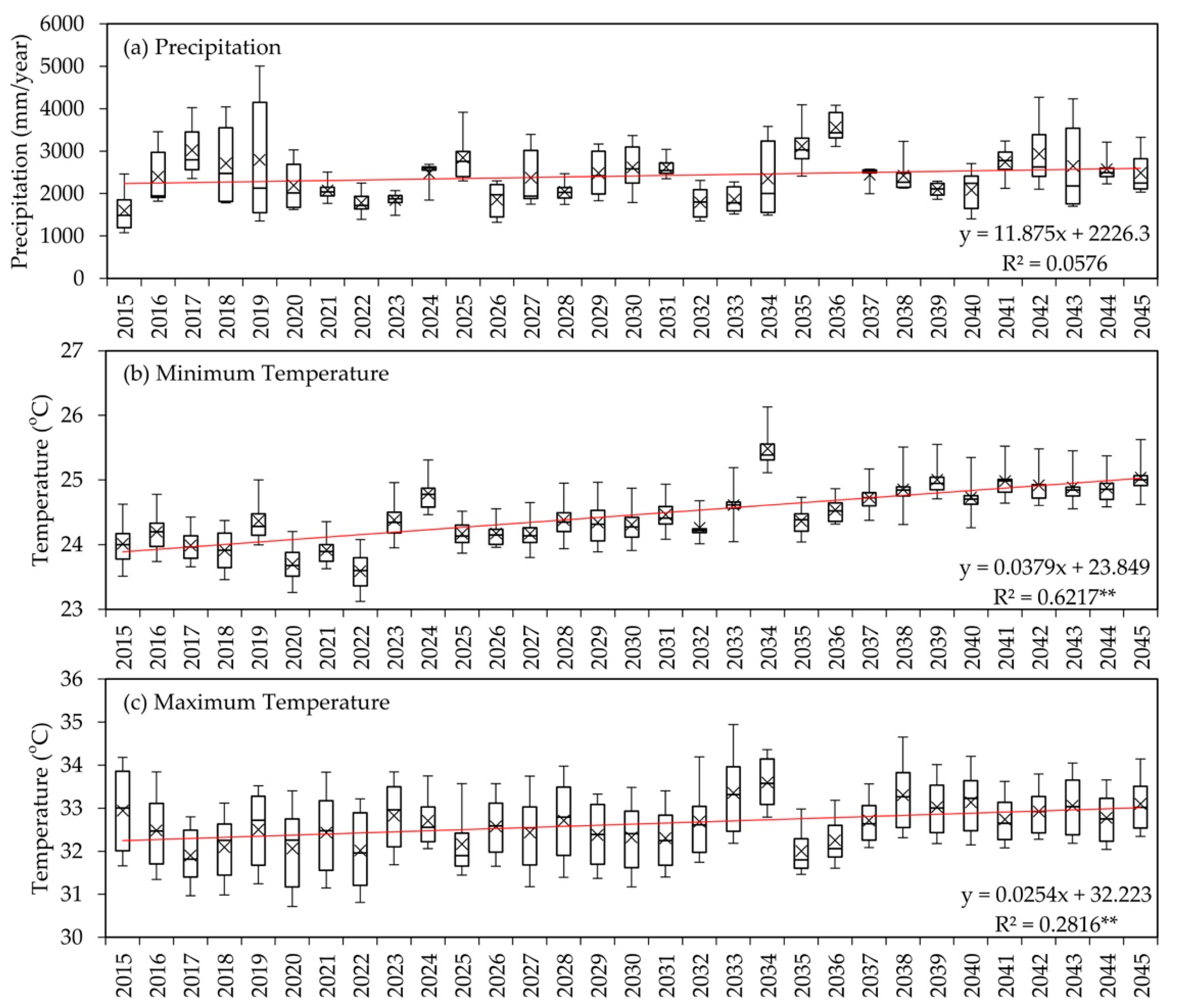
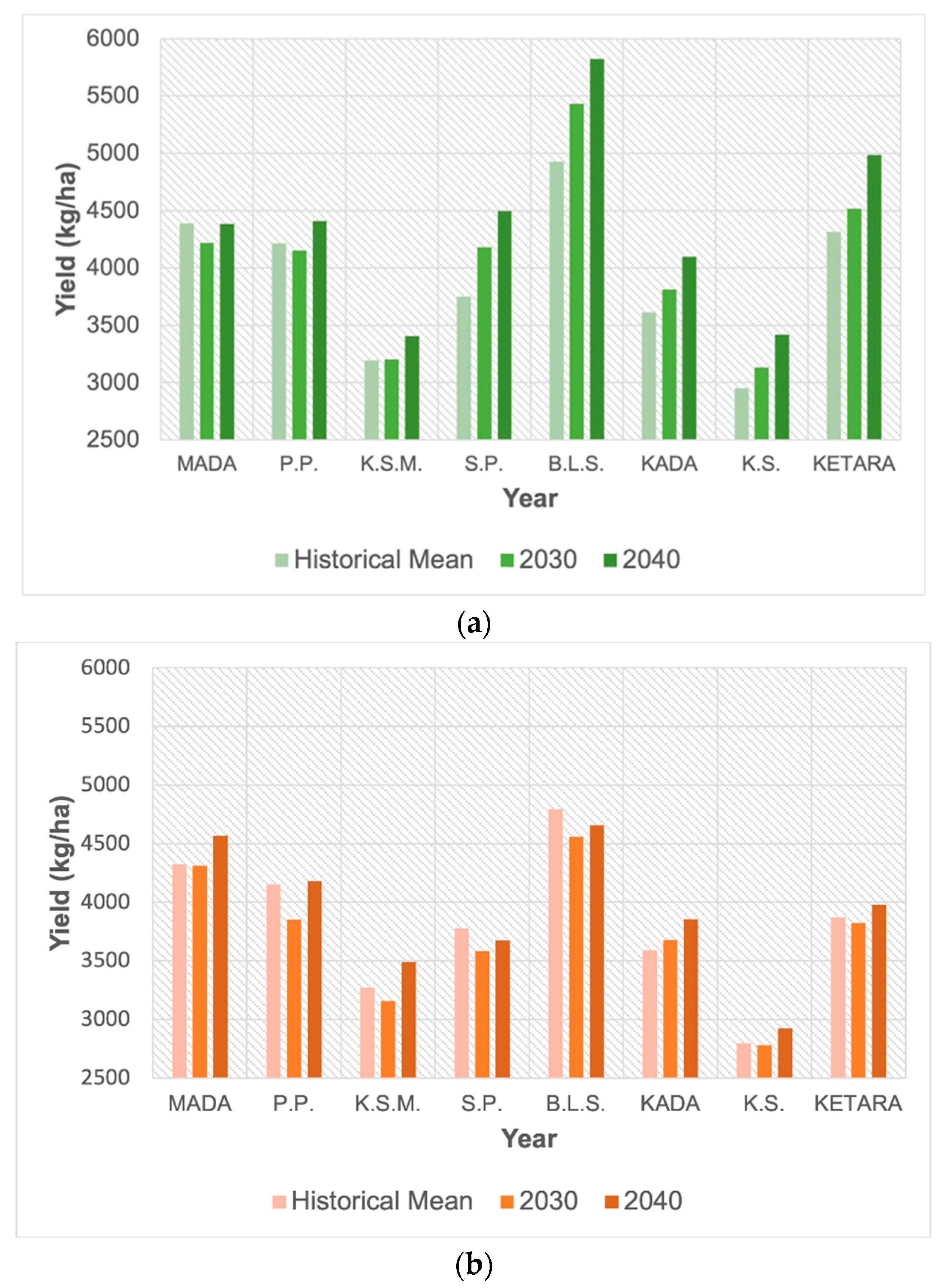
3.4. Projection of Future Yield with Climate Change

The projected climate change for 2030 and 2040 is based on the HadGEM3 model, as shown in Table 3. The projected changes are relative to the historical mean values of data used in this study. The projected scenario shown in Table 3 is assumed to be the same for the main season and off-season. The minimum and maximum temperature changes are shown in degrees Celsius, while the projected changes in precipitation are shown as percentages. The projected climate values were substituted into Model 2 to forecast the future rice yield under the projected climate change scenario. As shown in Table 8, the historical mean indicates the mean of the data used in this study (for the 1987–2017 period).
The forecasted values measure projected changes in the dependent variable as a function of changes in a specific explanatory variable while keeping other covariates constant. The results indicate that both MADA and P.P. were the only areas that would experience a slight decrease in rice yield during the main season. By the year 2030, MADA’s yield is projected to decline by −3.81%, followed by −0.02% over the following decade. Conversely, P.P. is expected to receive a positive effect by 2040 after experiencing a slight decrease in yield by 2030. By the year 2040, S.P. is expected to record the highest increase (19.85%) compared to the baseline average, followed by B.L.S. (18.12%).
The projected changes for off-season yield were very different compared to those for the main season. By the year 2030, rice yield in seven granary areas is expected to decline by −0.3 to −7.2%. P.P. would be the most affected granary area, followed by S.P., B.L.S., KSM, and KETARA. MADA would be the least affected area, followed by KS. Only KADA is projected to have increased rice yield over the next two decades. By the year 2040, all granary areas except S.P. and B.L.S. are projected to experience a positive effect when compared to the baseline average.
As shown in Figure 4a, the overall combined effects of increased temperature and decreased precipitation by 2030 (refer to Table 3) are likely to reduce rice yield in the main season in MADA and P.P. Even KSM would be affected by an increase in temperature and decrease in precipitation since yield is expected to increase marginally. However, an increase in precipitation by 2040 would reduce the effects of increased temperature since all granary areas are expected to record an increase in yield. Figure 4b indicates that the total effects of increased temperature and decreased or increased precipitation by 2030 would bring negative effects in all areas except for KADA. In KADA, an increase in precipitation of approximately 16% would help to reduce the effects of increased temperature. In the following decade, the effects of increased precipitation would allow the granary areas to increase their production per hectare, although the yield would remain below the baseline average in B.L.S. and S.P.
Based on Figure 4a,b, farmers in MADA, P.P. and K.S.M. would be the most affected since yield is expected to decrease in the coming decades. Conversely, the other five granaries are likely to benefit since the increase in yield during the main season is greater than the decrease in yield during the off-season. This could ultimately outweigh the rice production loss in MADA, P.P. and K.S.M. if one were to view this context from the ‘national production’ perspective. Nevertheless, using this perspective would certainly be unjust. That is to say, the majority of small farmers in these areas are just slightly above the poverty line and remain vulnerable to changes in farm productivity and income [9]. Hence, the results of this study undoubtedly reflect the importance of location-specific adaptation, which has not been observed in the other previous studies [15,16]. Moreover, location-specific factors [29] such as climate conditions over the next decade will further increase the variability of rice yield among granaries and between cropping seasons.
It is important to note that smaller countries in Southeast Asia, such as Malaysia, are expected to meet a rising proportion of their future cereal consumption (e.g., rice) through purchases from the international market [58]. Presently, Malaysia imports 30% of its rice to fulfill domestic consumption. Even if Malaysia is not a net importer of rice, retaining a long-term positive trend of rice production is critical to reducing the reliance on imports. Such an effort is not only vital to small farmers’ livelihoods but—most importantly—food security. Domestic rice production is critical to preventing the country from experiencing another serious shortage of supply due to a future global food crisis. Although the majority of rice production is concentrated in developing Southeast Asian countries, rising global rice prices are being transmitted into higher domestic rice prices, with the rise in domestic prices outpacing the rise in international prices in some countries [59]. Thus, government efforts to increase domestic rice production must be continued despite the challenges brought by the impacts of climate change.

4. Conclusions

Changes in climatic patterns would severely impact Malaysia’s rice production [4,9,10]. Thus, investigations related to the impact of climate change on rice yield are vital because rice is an important staple food for Malaysians. This study examined the impact of climate change on rice yield using a panel approach based on the LSDV model with PCSEs and using data from 1987 to 2017 on eight granary areas in Peninsular Malaysia.
The key findings show that climate variables significantly affect rice yield. Notably, while cultivated area size shows a positive impact on rice yield in both seasons, the magnitude of the impact is greater during the off-season. This suggests that by increasing the cultivation area size during the off-season, the effect on yield would be significant [9]. Rice yield is only negatively affected by precipitation during the main season since this season is also known as the wet season. Increased precipitation would lead to flooding, which usually occurs during this season. Instead, the minimum temperatures in the main season and off-season may experience inverse effects. Moreover, the main season is likely to experience a positive effect, while the off-season may experience the opposite effect. Lastly, maximum temperature adversely impacts rice yield in both seasons; however, the magnitude of the impact is greater during the off-season.
Upon simulating impacts under the HadGEM3 scenario, climate change was projected to reduce rice yield during the off-season by 2030. The P.P. granary area will be most affected, followed by S.P. and B.L.S. All of the remaining granary areas except KADA are also projected to encounter negative effects by 2030. By 2040, six granaries are predicted to gain positive effects, while the remaining two granaries (i.e., S.P. and B.L.S.) would likely experience negative effects. Hence, adaptation action measures must focus on the off-season period, particularly for B.L.S. and S.P. Such adaptation measures would include improving the existing irrigation infrastructure [60] (particularly during the off-season) and introducing high-temperature stress-tolerant rice cultivars while improving crop disease and pest management [61]. Although studies have shown that climate change could exaggerate pest and disease occurrence [30], this was not observed in our study. In summary, farm-level adaptations are crucial in enhancing farmers’ adaptive capacities and promoting long-term agricultural sustainability [62,63].

Author Contributions

Conceptualization, R.B.R.F.; Data curation, P.S.F. and R.B.R.F.; Formal analysis, B.T.T., R.B.R.F. and M.L.T.; Funding acquisition, R.B.R.F.; Investigation, B.T.T. and R.B.R.F.; Methodology, P.S.F., R.B.R.F. and M.L.T.; Project administration, R.B.R.F.; Resources, R.B.R.F.; Software, B.T.T. and M.L.T.; Supervision, P.S.F.; Validation, P.S.F. and R.B.R.F.; Writing—original draft, B.T.T. and R.B.R.F.; Writing—review and editing, R.B.R.F. and M.S.G. All authors have read and agreed to the published version of the manuscript.

Funding

This research was funded by the Ministry of Higher Education of Malaysia, grant number FRGS-203.PSOSIAL.6711692. CMIP6 climate data collection and bias correction were funded under the NEWTON-NERC grant by the Ministry of Higher Education Malaysia, grant number 203.PHUMANITI.6780001” and the NERC, grant number NE/S002707/1 with the project entitled-IMpacts of PRecipitation from Extreme StormS, Malaysia (IMPRESS-MALAYSIA).

Institutional Review Board Statement

Not applicable.

Informed Consent Statement

Not applicable.

Data Availability Statement

Not applicable.

Conflicts of Interest

The authors declare no conflict of interest. The funders had no role in the design of the study, in the collection, analyses, or interpretation of data, in the writing of the manuscript, or in the decision to publish the results.

References

  1. Brown, S.J.; Caesar, J.; Ferro, C.A.T. Global Changes in Extreme Daily Temperature Since 1950. J. Geophys. Res. Atmos. 2008, 113, D05115. [Google Scholar] [CrossRef] [Green Version]
  2. United Nations. The Sustainable Development Goals Report 2020; United Nations: New York, NY, USA, 2020; ISBN 978-92-1-004960-3. [Google Scholar]
  3. Arnell, N.W.; Lowe, J.A.; Challinor, A.J.; Osborn, T.J. Global and regional impacts of climate change at different levels of global temperature increase. Clim. Chang. 2019, 155, 377–391. [Google Scholar] [CrossRef] [Green Version]
  4. Firdaus, R.B.R.; Tan, M.L.; Rahmat, S.R.; Gunaratne, M.S. Paddy, Rice and Food Security in Malaysia: A Review of Climate Change Impacts. Cogent Soc. Sci. 2020, 6, 1818373. [Google Scholar] [CrossRef]
  5. Lobell, D.B.; Burke, M.B.; Tebaldi, C.; Mastrandrea, M.D.; Falcon, W.P.; Naylor, R.L. Prioritizing Climate Change Adaption Needs for Food Security in 2030. Science 2008, 319, 607–610. [Google Scholar] [CrossRef]
  6. Rosenzweig, C.; Elliott, J.; Deryng, D.; Ruane, A.C.; Müller, C.; Arneth, A.; Jones, J.W. Assessing Agricultural Risks of Climate Change in the 21st Century in a Global Gridded Crop Model Intercomparison. Proc. Natl. Acad. Sci. USA 2014, 111, 3268–3273. [Google Scholar] [CrossRef] [PubMed] [Green Version]
  7. Fischer, G.; Shah, M.; Tubiello, F.N.; van Velhuizen, H. Socio-economic and climate change impacts on agriculture: An integrated assessment, 1990–2080. Phil. Trans. R. Soc. B 2005, 360, 2067–2083. [Google Scholar] [CrossRef]
  8. Shrestha, S.; Deb, P.; Bui, T.T.T. Adaptation Strategies for Rice cultivation under Climate Change in Central Vietnam. Mitig. Adap. Strateg. Glob. Chang. 2016, 21, 15–37. [Google Scholar] [CrossRef]
  9. Firdaus, R.B.R.; Ibrahim, A.Z.; Siwar, C.; Jaafar, A.H. The Livelihood of Paddy Farmers in Facing Challenges of Climatic Change: The Role of Government Intervention Through Paddy Price Subsidy Scheme. Kaji. Malays. 2014, 32, 73. [Google Scholar]
  10. Azdawiyah, A.T.; Zabawi, A.G.M.; Hariz, A.R.M.; Fairuz, M.S.M.; Fauzi, J.; Faisal, M.M.S. Simulating Climate Change Impact on Rice Yield in Malaysia Using DSSAT 4.5: Shifting Planting Date as an Adaptation Strategy. NIAES Ser. 2016, 6, 115–125. [Google Scholar]
  11. Gupta, S.; Sen, P.; Srinivasan, S. Impact of Climate Change on the Indian Economy: Evidence from Food Grain Yields. Clim. Chang. Econ. 2014, 5, 1450001. [Google Scholar] [CrossRef] [Green Version]
  12. Poudel, S.; Kotani, K. Climatic impacts on crop yield and its variability in Nepal: Do they vary across seasons and altitudes? Clim. Chang. 2013, 116, 327–355. [Google Scholar] [CrossRef]
  13. Thuy, N.N.; Anh, H.H. Vulnerability of Rice Production in Mekong River Delta under Impacts from Floods, Salinity and Climate Change. Int. J. Adv. Sci. Eng. Inf. Technol. 2015, 5, 272–279. [Google Scholar] [CrossRef]
  14. Parker, L.; Bourgoin, C.; Martinez-Valle, A.; Laderach, P. Vulnerability of the agricultural sector to climate change: The development of a pantropical Climate Risk Vulnerability Assessment to inform sub-national decision making. PLoS ONE 2019, 14, e0213641. [Google Scholar] [CrossRef] [PubMed] [Green Version]
  15. Vaghefi, N.; Shamsudin, M.N.; Radam, A.; Rahim, K.A. Impact of climate change on food security in Malaysia: Economic and policy adjustments for rice industry. J. Integr. Environ. Sci. 2016, 13, 19–35. [Google Scholar] [CrossRef]
  16. Alam, M.M.; Siwar, C.; Talib, B.; Toriman, M.E.B. Impacts of Climatic Changes on Paddy Production in Malaysia: Micro Study on I.A.D.A. at North West Selangor. Res. J. Environ. Earth Sci. 2014, 6, 251–258. [Google Scholar] [CrossRef]
  17. Petersen, L.K. Impact of Climate Change on Twenty-First Century Crop Yields in the US. Climate 2019, 7, 40. [Google Scholar] [CrossRef] [Green Version]
  18. Muehe, E.M.; Wang, T.; Kerl, C.F.; Planer-Friedrich, B.; Fendorf, S. Rice production threatened by coupled stresses of climate and soil arsenic. Nat. Commun. 2019, 10, 4985. [Google Scholar] [CrossRef] [PubMed] [Green Version]
  19. Wang, W.; Yuan, S.; Wu, C.; Yang, S.; Zhang, W.; Xu, Y.; Gu, J.; Zhang, H.; Wang, Z.; Yang, J.; et al. Field experiments and model simulation based evaluation of rice yield response to projected climate change in Southeastern China. Sci. Total Environ. 2021, 721, 143206. [Google Scholar] [CrossRef]
  20. Ujiie, K.; Ishimaru, K.; Hirotsu, N.; Nagasaka, S.; Miyakoshi, Y.; Ota, M.; Tokida, T.; Sakai, H.; Usui, Y.; Ono, K.; et al. How elevated CO2 affects our nutrition in rice, and how we can deal with it. PLoS ONE 2019, 14, e0212840. [Google Scholar] [CrossRef]
  21. Zhu, C.; Kobayashi, K.; Loladze, I.; Zhu, J.; Jiang, Q.; Xu, X.; Liu, G.; Seneweera, S.; Ebi, K.L.; Drewnowski, A.; et al. Carbon dioxide (CO2) levels this century will alter the protein, micronutrients, and vitamin content of rice grains with potential health consequences for the poorest rice-dependent countries. Sci. Adv. 2018, 4, eaaq1012. [Google Scholar] [CrossRef] [Green Version]
  22. Blanc, E.; Reilly, J. Approaches to Assessing Climate Change Impacts on Agriculture: An Overview of the Debate. Rev. Environ. Econ. Policy 2017, 11, 247–257. [Google Scholar] [CrossRef] [Green Version]
  23. Welch, J.R.; Vincent, J.R.; Auffhammer, M.; Moya, P.F.; Dobermann, A.; Dawe, D. Rice Yields in Tropical/Subtropical Asia Exhibit Large but Opposing Sensitivities to Minimum and Maximum Temperatures. Proc. Natl. Acad. Sci. USA 2010, 107, 14562–14567. [Google Scholar] [CrossRef] [Green Version]
  24. Sarker, M.A.R.; Alam, K.; Gow, J. Assessing the Effects of Climate Change on Rice Yields: An Econometric Investigation Using Bangladeshi Panel Data. Econ. Anal. Policy 2014, 44, 405–416. [Google Scholar] [CrossRef]
  25. Mahrous, W. Climate Change and Food Security in E.A.C. Region: A Panel Data Analysis. Rev. Econ. Pol. Sci. 2019, 4, 270–284. [Google Scholar] [CrossRef] [Green Version]
  26. Kabir, M.H. Impacts of Climate Change on Rice Yield and Variability: An Analysis of Disaggregate Level in the Southwestern part of Bangladesh especially Jessore and Sathkhira Districts. J. Geogr. Nat. Disast. 2015, 5, 148. [Google Scholar] [CrossRef] [Green Version]
  27. Tan, M.L.; Juneng, L.; Tangang, F.T.; Chung, J.X.; Firdaus, R.B.R. Changes in Temperature Extremes and Their Relationship with ENSO in Malaysia from 1985 to 2018. Int. J. Climatol. 2020, 41, E2564–E2580. [Google Scholar] [CrossRef]
  28. Suhaila, J.; Jemain, A.A. Spatial Analysis of Daily Rainfall Intensity and Concentration Index in Peninsular Malaysia. Theor. Appl. Climatol. 2012, 108, 235–245. [Google Scholar] [CrossRef]
  29. Khazanah Research Institute. The Status of the Paddy and Rice Industry in Malaysia; Khazanah Research Institute: Kuala Lumpur, Malaysia, 2019; ISBN 978-967-16335-7-1. [Google Scholar]
  30. Firdaus, R.B.R.; Gunaratne, M.S.; Rahmat, S.R.; Kamsi, N.S. Does Climate Change Only Affect Food Availability? What Else Matters? Cogent Food Agric. 2019, 5, 1707607. [Google Scholar] [CrossRef]
  31. Firdaus, R.B.R.; Samsurijan, M.S.; Singh, P.S.J.; Yahaya, M.H.; Latiff, A.R.A.; Vadevelu, K. Impact of Climate Change on Agriculture based on the Crop Growth Simulation (C.G.S.) Model. Geogr. Malays. J. Soc. Space 2018, 14, 53–66. [Google Scholar] [CrossRef]
  32. Geng, X.; Wang, F.; Ren, W.; Hao, Z. Climate Change Impacts on Winter Wheat Yield in Northern China. Adv. Meteorol. 2019, 2019, 2767018. [Google Scholar] [CrossRef] [Green Version]
  33. Schierhorn, F.; Hofmann, M.; Adrian, I.; Bobojonov, I.; Muller, D. Spatially Varying Impacts of Climate Change on Wheat and Barley Yields in Kazakhstan. J. Arid Environ. 2020, 178, 104164. [Google Scholar] [CrossRef]
  34. Baltagi, B.H.; Kao, C.; Peng, B. Testing Cross-Sectional Correlation in Large Panel Data Models with Serial Correlation. Econometrics 2016, 4, 44. [Google Scholar] [CrossRef]
  35. Born, B.; Breitung, J. Testing for Serial Correlation in Fixed-Effects Panel Data Models. Econom. Rev. 2016, 35, 1290–1316. [Google Scholar] [CrossRef] [Green Version]
  36. Pesaran, M.H. Testing Weak Cross-Sectional Dependence in Large Panels. Econom. Rev. 2015, 34, 1089–1117. [Google Scholar] [CrossRef] [Green Version]
  37. Maddala, G.S.; Wu, S. A Comparative Study of Unit Root Tests with Panel Data and a New Simple Test. Oxf. Bull. Econ. Stat. 1999, 61, 631–652. [Google Scholar] [CrossRef]
  38. Pesaran, M.H. A Simple Panel Unit Root Test in the Presence of Cross Section Dependence. J. Appl. Econom. 2007, 22, 265–312. [Google Scholar] [CrossRef] [Green Version]
  39. Haarsma, R.J.; Roberts, M.J.; Vidale, P.L.; Senior, C.A.; Bellucci, A.; Bao, Q.; Chang, P.; Corti, S.; Fučkar, N.S.; Guemas, V.; et al. High-Resolution Model Intercomparison Project (HighResMIP v1.0) for CMIP6. Geosci. Model. Dev. 2016, 9, 4185–4208. [Google Scholar] [CrossRef] [Green Version]
  40. Liang, J.; Catto, J.L.; Hawcroft, M.; Hodges, K.I.; Tan, M.L.; Haywood, J.M. Climatology of Borneo Vortices in the HadGEM3-GC31 General Circulation Model. J. Clim. 2021, 34, 3401–3419. [Google Scholar] [CrossRef]
  41. Tan, M.L.; Liang, J.; Samat, N.; Chan, N.W.; Haywood, J.M.; Hodges, K.I. Hydrological Extremes Responses to Climate Change in the Kelantan River Basin, Malaysia, based on the CMIP6 HighResMIP experiments. Water 2021, 13, 1472. [Google Scholar] [CrossRef]
  42. Pesaran, M.H. General Diagnostic Tests for Cross Section Dependence in Panels. Empir. Econ. 2021, 60, 13–50. [Google Scholar] [CrossRef]
  43. Hoechle, D. Robust Standard Errors for Panel Regressions with Cross-Sectional Dependence. Stata J. 2007, 7, 281–312. [Google Scholar] [CrossRef] [Green Version]
  44. Park, R.W. Efficient Estimation of a System of Regression Equations when Disturbances are Both Serially and Contemporaneously Correlated. J. Am. Stat. Assoc. 1967, 62, 500–509. [Google Scholar] [CrossRef]
  45. Rahmat, S.R.; Firdaus, R.B.R.; Shaharudin, S.M.; Ling, L.Y. Leading Key Players and Support System in Malaysian Paddy Production Chain. Cogent Food Agri. 2019, 5, 1708682. [Google Scholar] [CrossRef]
  46. Reilly, J.; Tubiello, F.; McCarl, B.; Abler, D.; Darwin, R.; Fuglie, K.; Hollinger, S.; Izaurralde, C.; Jagtap, S.; Jones, J.; et al. U.S. agriculture & climate change: New results. Clim. Chang. 2003, 57, 43–69. [Google Scholar] [CrossRef]
  47. Long, S.P.; Ainsworth, E.A.; Rogers, A.; Ort, D.R. Rising atmospheric carbon dioxide: Plants face the future. Annu. Rev. Plant. Biol. 2004, 55, 591–628. [Google Scholar] [CrossRef] [PubMed]
  48. Long, S.P.; Ainsworth, E.A.; Leakey, A.D.B.; Morgan, P.B. Global food insecurity: Treatment of major food crops with elevated carbon dioxide or ozone under large-scale fully open-air conditions suggests recent models may have overestimated future yields. Phil. Trans. R. Soc. B 2005, 360, 2011–2020. [Google Scholar] [CrossRef]
  49. Cline, W.R. Global Warming and Agriculture: Impact Estimates by Country; Peterson Institute for International Economics: Washington, DC, USA, 2007. [Google Scholar]
  50. Long, S.P.; Ainsworth, E.A.; Leakey, A.D.B.; Nosberger, J.; Ort, D.R. Food for thought: Lower than expected crop yield stimulation with rising CO2 concentrations. Science 2006, 312, 1918–1921. [Google Scholar] [CrossRef]
  51. Easterling, W.E.; Aggarwal, P.K.; Batima, P.; Brander, K.M.; Erda, L.; Howden, S.M.; Kirilenko, A.P.; Morton, J.; Soussana, J.-F.; Schmidhuber, J.; et al. Food, fibre and forest products. In Climate Change 2007: Impacts, Adaptation and Vulnerability. Contribution of Working Group II to the Fourth Assessment Report of the Intergovernmental Panel on Climate Change; Parry, M.L., Canziani, O.F., Palutikof, J.P., van der Linden, P.J., Hanson, C.E., Eds.; Cambridge University Press: Cambridge, UK, 2007; pp. 273–313. [Google Scholar]
  52. Rötter, R.P.; Carter, T.R.; Olesen, J.E.; Porter, J.R. Crop–climate models need an overhaul. Nat. Clim. Chang. 2011, 1, 175–177. [Google Scholar] [CrossRef]
  53. Toreti, A.; Deryng, D.; Tubiello, F.N.; Müller, C.; Kimball, B.A.; Moser, G.; Boote, K.; Asseng, S.; Pugh, T.A.M.; Vanuytrecht, E.; et al. Narrowing Uncertainties in the Effects of Elevated CO2 on Crops. Nat. Food 2020, 1, 775–782. [Google Scholar] [CrossRef]
  54. Hasegawa, T.; Sakai, H.; Tokida, T.; Nakamura, H.; Zhu, C.; Usui, Y.; Yoshimoto, M.; Fukuoka, M.; Wakatsuki, H.; Katayanagi, N.; et al. Rice Cultivar Responses to Elevated CO2 at Two Free–air CO2 Enrichment (FACE) Site in Japan. Funct. Plant Biol. 2013, 40, 148–159. [Google Scholar] [CrossRef] [Green Version]
  55. Kimball, B.A. Crop Responses to Elevated CO2 and Interactions with H2O, N, and Temperature. Curr. Opin. Plant Biol. 2016, 31, 36–43. [Google Scholar] [CrossRef]
  56. Hasegawa, T.; Li, T.; Yin, X.; Zhu, Y.; Boote, K.; Baker, J.; Bregaglio, S.; Buis, S.; Confalonieri, R.; Fugice, J.; et al. Causes of variation among rice models in yield response to CO2 examined with Free-Air CO2 Enrichment and growth chamber experiments. Sci. Rep. 2017, 7, 14858. [Google Scholar] [CrossRef] [PubMed] [Green Version]
  57. Lv, C.; Huang, Y.; Sun, W.; Yu, L.; Zhu, J. Response of rice yield and yield components to elevated [CO2]: A synthesis of updated data from FACE experiments. Eur. J. Agron. 2020, 112, 125961. [Google Scholar] [CrossRef]
  58. Dyson, T. World food trends: A neo-Malthusian prospect? Proc. Am. Philos. Soc. 2001, 145, 438–455. [Google Scholar] [PubMed]
  59. Asian Development Bank. Global Food Price Inflation and Developing Asia Special Report; Asian Development Bank: Manila, Philippines, 2011; ISBN 978-92-9092-282-7. [Google Scholar]
  60. Toriman, M.E.; Mokhtar, M. Irrigation: Types, Sources and Problems in Malaysia. In Irrigation Systems and Practices in Challenging Environments, 1st ed.; Lee, T.S., Ed.; IntechOpen: London, UK, 2012. [Google Scholar] [CrossRef]
  61. Sekhar, C.S.C. Climate Change and Rice Economy in Asia: Implications for Trade Policy; Food and Agriculture Organization: Rome, Italy, 2018. [Google Scholar]
  62. Yasar, M.; Siwar, C.; Firdaus, R.B.R. Assessing Paddy Farming Sustainability in the Northern Terengganu Integrated Agricultural Development Area (IADA KETARA): A Structural Equation Modelling Approach. Pac. Sci. Rev. B Humanit. Soc. 2015, 1, 71–75. [Google Scholar] [CrossRef] [Green Version]
  63. Firdaus, R.B.R.; Samsurijan, M.S.; Singh, P.S.J.; Yahaya, M.H.; Latiff, A.R.A.; Rahmat, S.R.; Vadevelu, K. Ke Arah Mencapai 100% Kadar Sara Diri (SSL) Beras: Satu Sasaran Realistik atau Retorik? In Proceedings of the Persidangan Kebangsaan Masyarakat, Ruang dan Alam Sekitar, USM, Pulau Pinang, Malaysia, 23–24 February 2017. [Google Scholar]
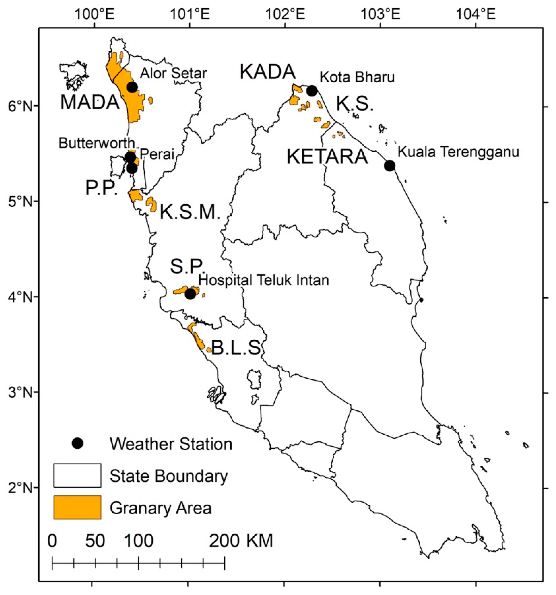
Figure 1. Locations of granary areas and weather stations.
Agriculture 11 00569 g001
Figure 2. Projection of mean annual maximum and minimum temperatures and precipitation for all granary areas (2015–2045). Linear regression analyses show a significant trend (** p < 0.05).
Agriculture 11 00569 g002
Figure 3. Comparison of historical changes over the 1987–2017 period by cropping season. (a) Average yield of eight granaries (mt/ha). (b) Average sum of precipitation (mm) with error bars showing one standard deviation. (c) Average minimum temperature (°C) with error bars are +/−0.2 °C. (d) Average maximum temperature (°C) with error bars are +/−0.2 °C.
Agriculture 11 00569 g003aAgriculture 11 00569 g003b
Figure 4. Forecasted yield in 2030 and 2040 relative to the sample means. (a) Main Season. (b) Off-Season.
Agriculture 11 00569 g004
Table 1. List of granary areas and weather stations.
Granary AreasWeather Stations
1.Muda Agricultural Development AuthorityMADAAlor Setar
2.Integrated Agricultural Development Area Pulau Pinang P.P.Butterworth
3.Integrated Agricultural Development Area KerianK.S.M.Perai
4.Integrated Agricultural Development Area Seberang PerakS.P.Hospital Teluk Intan
5.Integrated Agricultural Development Area Barat Laut Selangor B.L.S.Hospital Teluk Intan
6.Kemubu Agricultural Development AuthorityKADAKota Bharu
7.Integrated Agricultural Development Area Kemasin SemarakK.S.Kota Bharu
8. Integrated Agricultural Development Area KETARAKETARAKuala Terengganu
Table 2. Variable description.
Type of
Variable
VariableDescription
DependentYield (kg/ha)Average yield per season
IndependentLand (ha)Total cultivated area per season
P (mm)Total precipitation per season
Tmin (°C)Average of daily minimum temperature per season
Tmax (°C)Average of daily maximum temperature per season
Table 3. Future climate scenario.
20302040
No.Station IDStation
Name
Min Temp.
(°C)
Max Temp.
(°C)
Changes in Precipitation
(% mm)
Min Temp.
(°C)
Max Temp.
(°C)
Changes in Precipitation
(% mm)
148603Alor Setar0.630.70−2.310.930.7215.04
241529Perai0.410.61−14.040.750.76−4.79
348620Teluk Intan0.610.711.000.970.859.73
448615Kota Bharu0.320.3515.910.740.7113.08
548602Butterworth0.410.59−15.800.720.72−4.11
648618Kuala Terengganu0.340.378.580.730.7615.80
Table 4. Descriptive statistics.
Granary AreasAnnual YieldPlanted AreaAnnual Total PrecipitationAnnual Mean Minimum TemperatureAnnual Mean Maximum Temperature
MADAMean4358.78192,180.302046.7024.0532.72
Std. Dev.546.943205.78287.170.360.36
P.P.Mean4180.0120,878.382263.4324.1332.05
Std. Dev.1270.182197.34293.890.450.35
K.S.M.Mean3234.2751,044.322146.0224.7332.24
Std. Dev.628.325277.8337.650.440.39
S.P.Mean3765.9317,782.202383.3523.7033.12
Std. Dev.627.664831.62423.330.600.48
B.LS.Mean4859.7236,649.882383.3523.7033.12
Std. Dev.822.841076.94423.330.600.48
KADAMean3622.2949,311.362599.4924.0631.46
Std. Dev.510.076193.62635.790.300.32
K.S.Mean2941.076455.102599.4924.0631.46
Std. Dev.587.131944.64635.790.300.32
KETARAMean4095.549342.382680.5524.1131.53
Std. Dev.1063.411084.46539.940.370.42
Table 5. Panel unit root test.
VariablesFisher-ADFPesaran Unit Root Test
Without TrendWith TrendWithout TrendWith Trend
Main SeasonLnYield41.32 ***
(>0.001)
61.07 ***
(>0.001)
−3.30 ***
(>0.001)
−2.082 **
(0.019)
Land53.20 ***
(>0.001)
50.18 ***
(>0.001)
−2.46 ***
(0.007)
−2.10 **
(0.018)
P115.28 ***
(>0.001)
109.30 ***
(>0.001)
−2.80 ***
(0.003)
−1.61 *
(0.054)
Tmin24.16 *
(0.086)
78.71 ***
(>0.001)
−3.17 ***
(0.001)
−1.65 *
(0.050)
Tmax110.61 ***
(>0.001)
90.69 ***
(>0.001)
−4.76 ***
(>0.001)
−4.82 ***
(>0.001)
Off-SeasonLnYield57.02 ***
(>0.001)
56.15 ***
(>0.001)
−7.11 ***
(>0.001)
−6.14 ***
(>0.001)
Land96.10 ***
(>0.001)
306.89 ***
(>0.001)
−2.88 ***
(>0.001)
−3.83***
(>0.001)
P120.87 ***
(>0.001)
91.75 ***
(>0.001)
−4.37 ***
(>0.001)
−2.75 ***
(0.003)
Tmin35.11 ***
(0.004)
98.82 ***
(>0.001)
−4.90 ***
(>0.001)
−3.61 ***
(>0.001)
Tmax85.18 ***
(>0.001)
73.96***
(>0.001)
−4.07 ***
(>0.001)
−5.08 ***
(>0.001)
*, ** and *** denotes significance levels at 10%, 5% and 1% respectively. Values in brackets represent the p-value.
Table 6. Diagnostic test results.
SeasonTypeBreusch-PaganWooldridgeCD
MainLinear0.69
(0.406)
10.769 **
(0.014)
6.66 ***
(>0.001)
Quadratic5.08 **
(0.024)
11.057 **
(0.013)
6.946 ***
(>0.001)
OffLinear12.77 ***
(>0.001)
11.461 **
(0.012)
8.049 ***
(>0.001)
Quadratic34.91 ***
(>0.001)
9.123 **
(0.019)
6.732 ***
(>0.001)
** and *** denotes significance levels at 5% and 1% respectively. Values in parenthesis are p-value.
Table 7. Model estimation with PCSE for main and off-season.
VariableMain SeasonOff-Season
Model 1Model 2Model 1Model 2
Coefficientp-ValueCoefficientp-ValueCoefficientp-ValueCoefficientp-Value
Constant5.431 ***>0.00124.732 0.5557.716 ***>0.001−22.1800.620
Land0.00001 ***0.0030.00008 ***0.0020.00002 ***0.007−3.14 × 10−60.889
P0.00004 0.217−0.0020.4150.00005 0.401−0.003 0.372
Tmin0.0998 ***0.0070.009 0.9970.109 **0.0180.031 0.988
Tmax0.125 0.557−1.108 0.438−0.069 * 0.0771.8720.320
Land2 −1.05 × 10−100.319 −1.90 × 10−100.063
P2−4.02 × 10−80.448−4.56 × 10−800.829
Tmin20.002 0.9600.085 ***0.008
Tmax20.021 0.2200.015 0.588
P × Tmin0.0001 **0.0440.0001 0.159
P × Tmax−0.00004 0.205−7.17 × 10−70.993
Tmin × Tmax−0.005 0.852−0.123 ***0.003
T-Stat231.040284.01141.38195.07
p-value>0.001>0.001>0.001>0.001
Adj. R20.9190.90780.85160.8236
*, ** and *** denotes significance levels at 10%, 5% and 1% respectively.
Table 8. Forecasted yield for the years 2030 and 2040 relative to the sample means.
SeasonGranary AreaHistorical MeanYear 2030Year 2040
MainMADA4386.654219.49(−3.81)4385.73(−0.02)
P.P.4212.194150.27(−1.47)4410.19(4.7)
K.S.M.3193.103201.12(0.25)3407.50(6.71)
S.P.3750.264179.25(11.44)4494.51(19.85)
B.L.S.4927.875434.14(10.27)5820.84(18.12)
KADA3612.133811.01(5.51)4098.23(13.46)
K.S.2949.523133.17(6.23)3417.32(15.86)
KETARA4312.484515.43(4.71)4986.26(15.62)
OffMADA4324.084311.01(−0.30)4565.69(5.59)
P.P.4151.713852.92−(7.2)4180.91(0.7)
K.S.M.3273.843155.74(−3.61)3492.12(6.67)
S.P.3779.843585.37(−5.14)3675.03(−2.77)
B.L.S.4792.654558.76(−4.88)4655.04(−2.87)
KADA3588.003680.55(2.58)3853.96(7.41)
K.S.2797.072779.44(−0.63)2922.28(4.48)
KETARA3870.583822.04(−1.25)3981.00(2.85)
Values in parenthesis are the percentage of change relative to the historical mean of yield.
Publisher’s Note: MDPI stays neutral with regard to jurisdictional claims in published maps and institutional affiliations.

