1. Introduction
The extent of food-insecure people in the world has decreased during the past decade but is estimated to still be more than 820 million [
1,
2]. With continued population growth, more food production will be required with lower resource inputs such as labor, fertilizer, water, and land. This is a challenge that cannot be met by focusing exclusively on increasing food production. As a result, reducing post-harvest loss has been recognized as a vital tool for meeting global food and energy needs [
1,
3]). Even grain that has been handled properly may develop adverse conditions due to insect infestations, moisture condensation, mold spoilage and weather effects. Monitoring grain conditions during aeration and storage is an important strategy to ensure grain quality and food safety.
Monitoring grain conditions is most useful when implemented in conjunction with grain management strategies to maintain the quality of grain and reduce or prevent post-harvest loss. One of the most popular post-harvest loss prevention technologies is grain aeration, which is commonly used in temperate climates such as the upper Midwest of the United States. Aeration reduces insect reproduction [
4] by reducing temperatures below the optimum for insect development, i.e., 28 °C to 38 °C [
5]. Once grain has been cooled below the lower limit for stored grain insects, i.e., 13 °C to 20 °C [
6], the risk of grain loss due to insect growth has been mitigated. The use of aeration is complicated by a number of factors, such as the suitability of weather conditions to achieve effective cooling, the need to control moisture content, and the desire to reduce fan run hours. For this reason, much research has been focused on developing effective algorithms to govern the operating systems of grain aeration fans [
7,
8,
9,
10,
11]. Many effective strategies, such as those utilized [
8], make use of information gathered from the grain mass to make aeration decisions. The effectiveness of these strategies depends on the location and number of sensors used to monitor the grain mass, and how representative those readings are of the entire grain mass. However, little research has been conducted to investigate how grain monitoring decisions, such as the number and placement of temperature sensors, can impact grain aeration efficacy.
The most common monitoring system currently used in stored grain bulks relies on steel cables equipped with thermocouple or thermistor type sensors placed 1.82–2.09 m (6–7 ft) apart. The cables are hung in a bin, silo, tank, or building from the roof supports. While temperature cables remain an important tool, they have several limitations and disadvantages. Grain is a good insulator, so sensors indicate temperature within a limited range and cables result in increased friction forces as the grain mass settles over time or is unloaded. This causes substantial loads on the roofs of grain structures, for example, as high as 4700 N (1056 lbs) in the unloading of a 279 MT silo [
12]. Particularly for large storage structures, roofs have to be properly engineered to carry the loading force associated with the number of cables needed to monitor a grain mass. Also, with time thermocouple-based temperature sensors can become inaccurate. Many older systems installed in silos have cables that no longer function reliably. Temperature sensors also do not give an indication of moisture content in the grain mass, an important factor for considering grain quality.
Companies selling temperature cables have specific recommendations for the number and location of cables for different storage structure types and sizes. They range from a minimum of a single cable placed in the center of a grain mass to a large number of cables supposedly covering 100% of a large grain mass. No scientific research has been found that documents the relationship between number and placement of sensors and those temperature readings versus actual temperatures in a stored grain mass, or how those readings would affect aeration strategies that utilize data from the grain mass.
Detecting a hotspot (i.e., high temperature as a result of grain spoilage) in a sensor’s range occurs only when the hotspot has grown large enough to begin being detected [
13]. Unfortunately, by the time hot spots are large enough to detect, significant damage to the grain mass has already occurred. Grain is a good thermal insulator, but a grain mass contains 35–40% air space, and thus the, sensors measure as much interstitial air conditions as actual grain temperature. Air movement can also be an important factor in determining how early hotspots might be detected. Ileleji et al., 2006 determined that temperature cable sensors 0.3 to 1 m distance from a developing “spoilage hotspot” were unable to detect increasing temperatures [
14]. According to Mills (1989), relative humidity and temperature sensors are sensitive to grain conditions at a distance of 30 to 60 cm [
15]. This poses a problem because many temperature cable companies advertise cable systems based on a percentage of the grain silo that is “covered” by the sensors with no indication of the length of time or amount of grain it would take for a hotspot a particular distance from a sensor to be detected.
Temperature cables are not commonly placed near the sidewalls of a storage structure, limiting the ability to reliably monitor the perimeter of the grain mass where external solar radiation substantially influences grain temperature and moisture changes which can cause wall caking and grain spoilage. This limits the likelihood that potential grain storage problems will be detected with temperature sensors in a timely manner as grain mass surface and perimeter areas are typically the first areas in the storage structure to be infested by insects.
A novel stored grain monitoring technology that allows for tracking temperature (see
Figure 1), relative humidity, and other factors wirelessly is being developed by at least one company (i.e., Amber Agriculture and others). Wireless technology offers a new option in grain storage management by allowing a variable number of sensors to be placed in the grain mass, and with a potentially random vertical and horizontal distribution. The sensors can be removed after grain storage with a simple sieve. A random horizontal distribution would have the advantage of placing sensors in vulnerable areas of the grain mass periphery that conventional cables sensors cannot reach. Wireless sensors will also allow for any number of sensors to be placed in the grain mass without negative consequences on roof structural integrity. However, there is a potential risk if sensors are distributed in ways that give an inaccurate representation of grain mass conditions, or if there is no way of knowing where exactly the wireless sensors end up in the grain mass when added to the grain flow during silo filling. Furthermore, if wireless sensor locations are randomly distributed, how would a stored grain manager know whether this distribution results in more or less representative temperature readings than those of traditional cable-based sensors, or improves aeration performance or how the distribution of these sensors can impact aeration performance?
The 3D MLP (Maier, Lawrence, Plumier) finite element model has been previously used to investigate stored grain ecosystems in a variety of situations [
8,
16,
17,
18]. It has the capacity to analyze the effects that changing sensor distributions have on aeration results by running multiple simulations with sensors distributed in ways consistent with the existing temperature cable technology and the randomized wireless sensor technology. The model also has the ability to simulate the effects of different aeration fan runtime choices made by stored grain managers.
The objectives of this research were to evaluate the effect of temperature sensor numbers and placement on aeration cooling of a stored grain mass utilizing three recommended temperature cable configurations and randomized horizontal placement of “wireless” sensors at fixed depths, and to investigate the impact of these configurations on interpreting grain conditions and associated aeration system operating decisions.
2. Materials and Methods
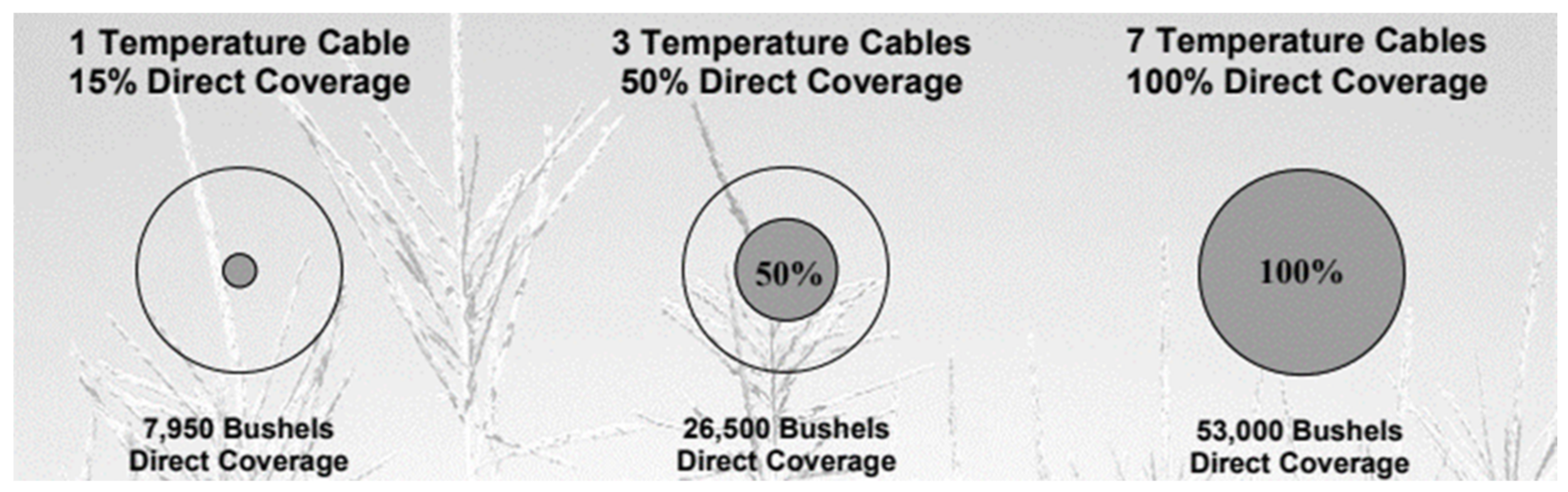
For the purpose of investigating the effect of the number and placement of temperature sensors on aeration cooling of a stored grain mass, the recommended configurations of one commercial supplier of temperature cable monitoring systems, i.e., Tri-States Grain Conditioning Inc. (Spirit Lake, IA, USA) were utilized. The three recommended temperature cable configurations were for a 1346 MT (53,000 bushel) silo holding peaked maize (see
Figure 2). In the first configuration, one cable is hung in the center of the silo and claims to monitor temperatures reliably in 201 MT (7950 bushels) of maize in the core, equivalent to 15% of the total grain mass. In the second configuration, three cables are hung in the silo, evenly spaced radially and 1/3 of the distance between the center and the wall of the silo. This placement claims to monitor temperatures reliably in 673 MT (26,500 bushels) of maize within a larger radius of the core, equivalent to 50% of the total grain mass. In the third configuration, seven cables are hung in the silo, with six cables evenly spaced radially and 2/3 of the distance between the center and the wall of the silo plus one cable in the center. This placement claims to monitor temperatures reliably in 1346 MT (53,000 bushels) of maize from core to wall of the silo, equivalent to 100% of the grain mass. These sensor distributions will be referred to as low, medium, and high. Each cable had six evenly spaced sensors 2.09 m apart (7 ft) from bottom to top. The silo specifications (14.6 m diameter, 10.1 m eave height, 14.6 m peak height) were used to create a mesh of elements for 3D simulation of a level stored grain mass using the Abaqus software with 2940 nodes. One year of hourly weather data (2014) (i.e., solar radiation, temperature, relative humidity, and wind speed) was acquired from the Iowa State Mesonet system (
https://mesonet.agron.iastate.edu, accessed on 9 September 2019), representing the aerated grain storage period in Ames, IA, USA.
In the first investigation, the effectiveness of each of the sensor cable configurations in representing the actual average conditions of the grain mass was analyzed during one year of aerated storage. The aeration strategy ran the fan whenever the center point of the grain mass was warmer than ambient temperature conditions. The fan was turned off whenever the temperature of the sensor in the middle of the grain mass was lower than the ambient air temperature. These aeration strategies are based on successful strategies discussed in Plumier (2018) [
9]. While the aeration simulations were identical in this trial, the results shown represent the values observed by monitoring the grain at positions reflective of the sensor locations in each of the three monitoring strategies described in
Figure 2, along with one labeled total that represents the temperature values reflected by averaging all 2940 nodes of the numerical solution.
For the second investigation, four aeration simulations were conducted where the aeration control strategy was dependent on the values observed by the sensor locations indicated by the three cable configurations depicted in
Figure 2. The aeration fan was turned on whenever the average temperature reported by all sensors for a particular cable configuration was greater than the ambient temperature, and that average grain temperature was above 0 °C. The fan was turned off whenever the average of the sensors was lower than the ambient air temperature. Results were analyzed for each of the three configurations as well as for the total that represents the average of the numerical solution.
The third analysis investigated aeration fans controlled by sensors placed randomly at horizontal locations, that is, in line with the potential new wireless sensor technology. To accomplish this, sensor locations in the code were placed at depths and in numbers that correspond to the sensor locations of the three cable configurations. The horizontal positioning of each of the nodes, however, was assigned using a random number generator. The same aeration strategy was used as in the previous analysis. Ten replicates of the aeration simulations were conducted with numbers corresponding to the low, medium, and high sensor distributions. The averages, standard deviations, and differences between the highest and lowest temperature values were reported.
In order to further investigate the difference between placing a cable in the center or the periphery, the single cable configuration was investigated by also placing it one-third and two-thirds of the distance to the silo wall and along the silo wall in the eastern direction.
3. Results
The three cable configurations purportedly represent “direct coverage” for 15%, 50%, and 100% of the grain mass with one, three, and seven cables, respectively. However, it is not known how far from a sensor a point in the grain mass can be located and still represent the same grain temperature as the sensor location. It is also unclear how these percentages were calculated given temperature sensor locations 2.09 m apart along with a cable and cable placement configurations. Based on the radius of a 1.05 m sphere around each sensor without overlap between sensor volumes, the three cable configurations would represent only 1.5%, 4.6%, and 10.8% of the grain mass, respectively. In order to achieve the claimed values, it is necessary to assume a radius of greater length (i.e., 2.23 m) than the distance between the sensors (i.e., 2.09 m) and overcount overlapped areas between sensor volumes. These assumptions would yield 15%, 45%, and 105% of the grain mass represented by the three respective cable configurations. However, this is clearly unrealistic, as there are locations in the grain mass that are not covered and some areas that are double or triple counted. From the perspective of a stored grain manager, this would not make any sense. As a matter of fact, it may give a false sense of security in terms of how quickly a temperature increase due to mold spoilage, for example, would be detected. Accounting for only the vertical overlap within each column, the representative grain mass volumes would reduce to less than 9.6%, 28.7%, and 66.9%, respectively, but the implication stated above remains. Thus, the subsequent simulation results were not presented and discussed in terms of these percentage values.
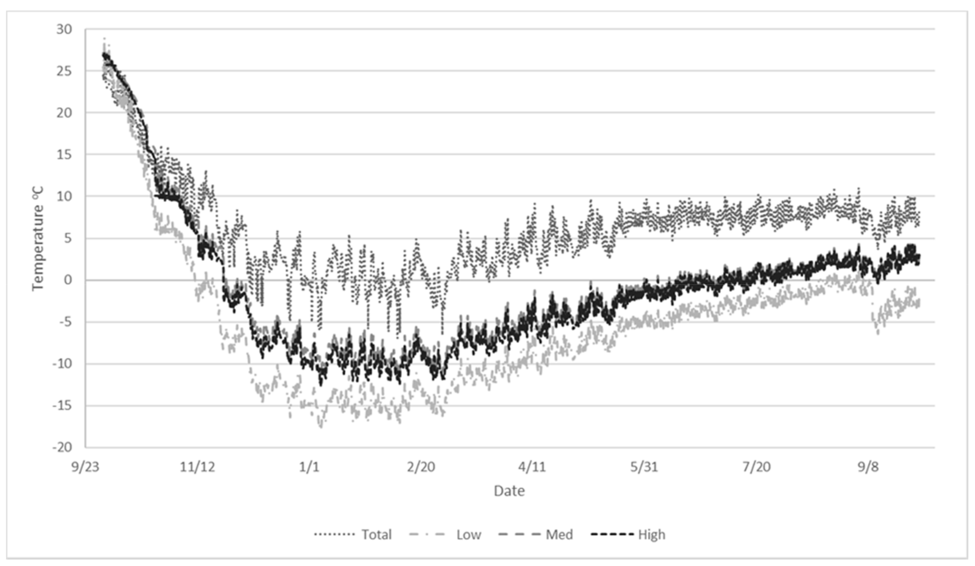
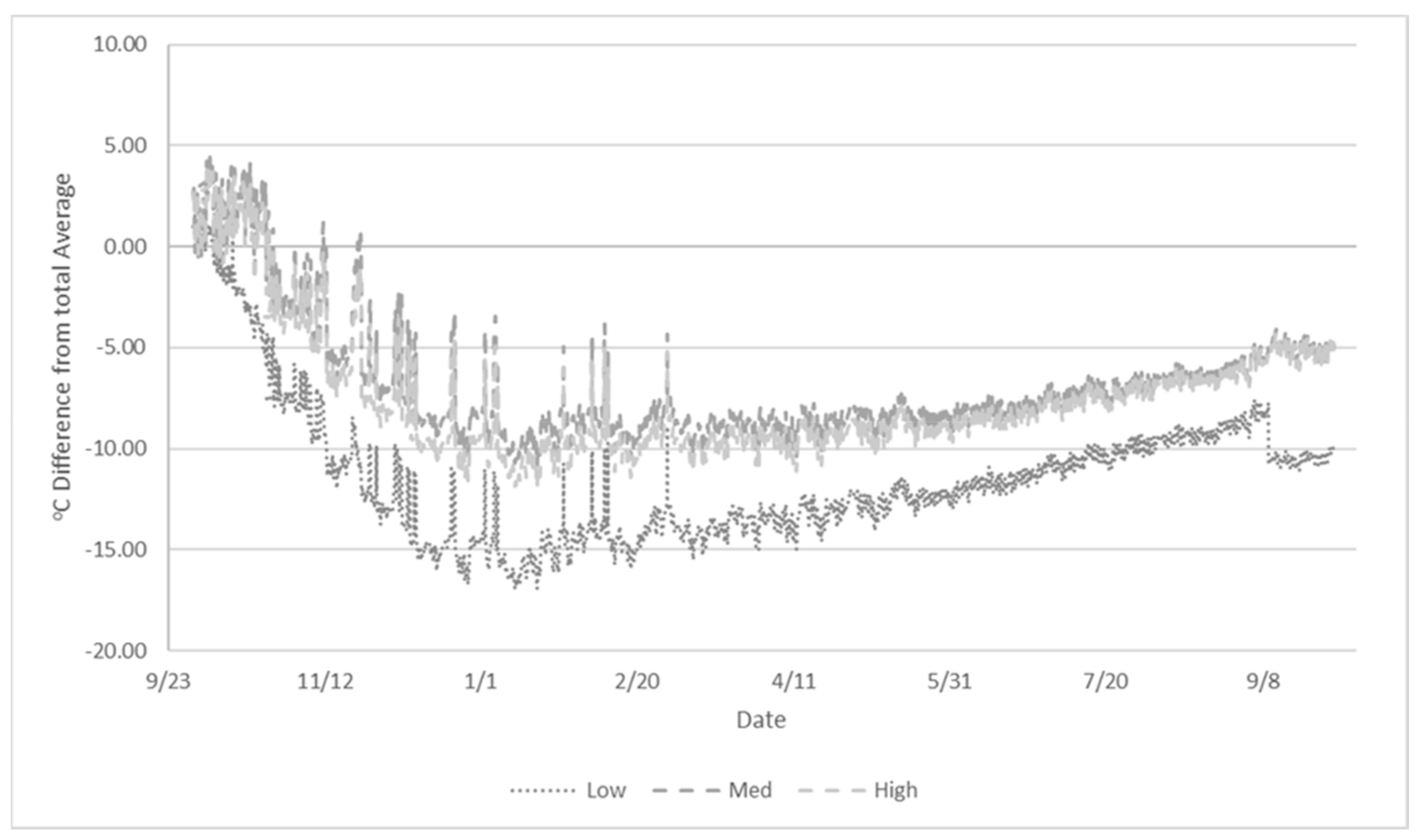
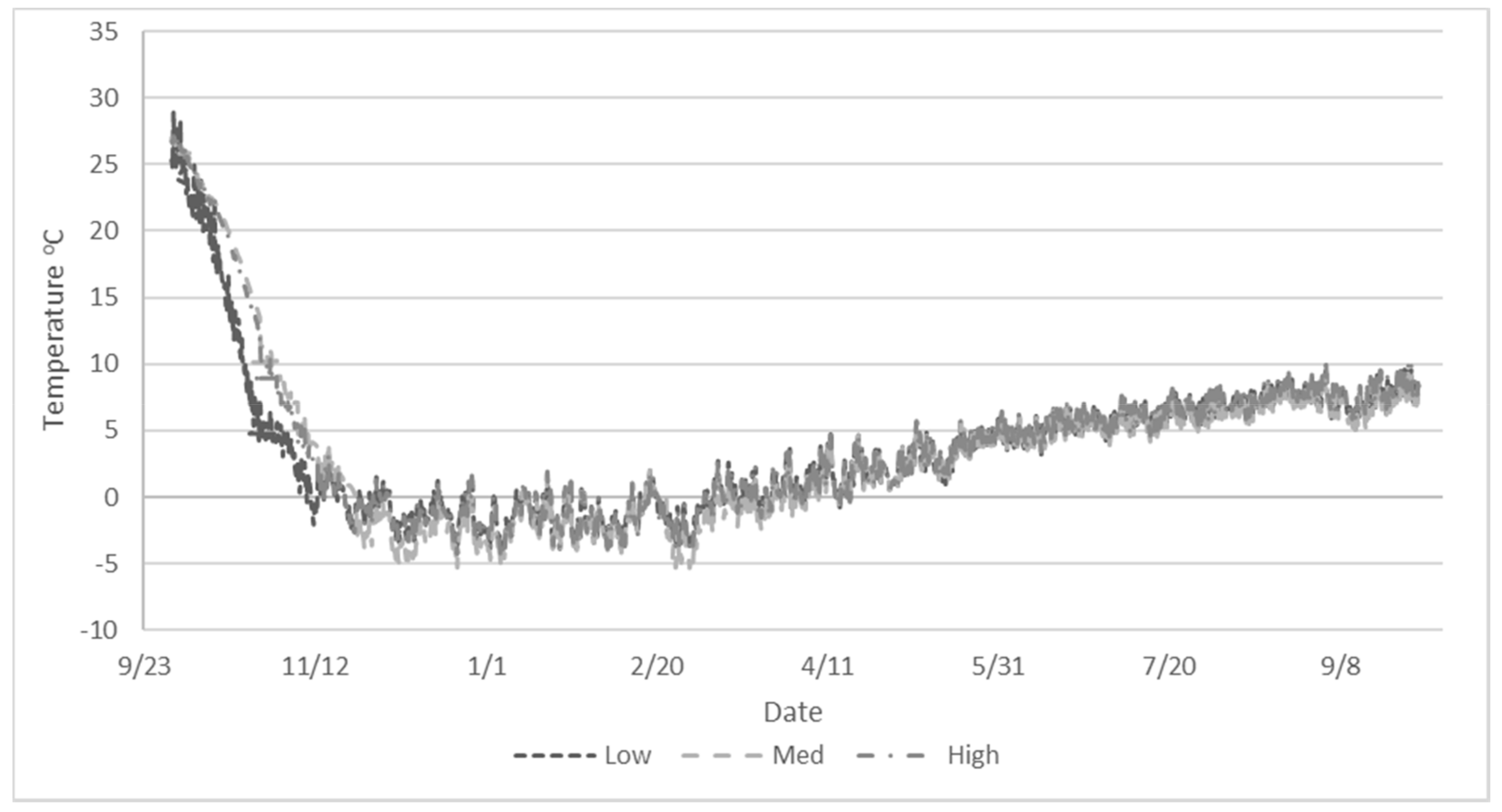
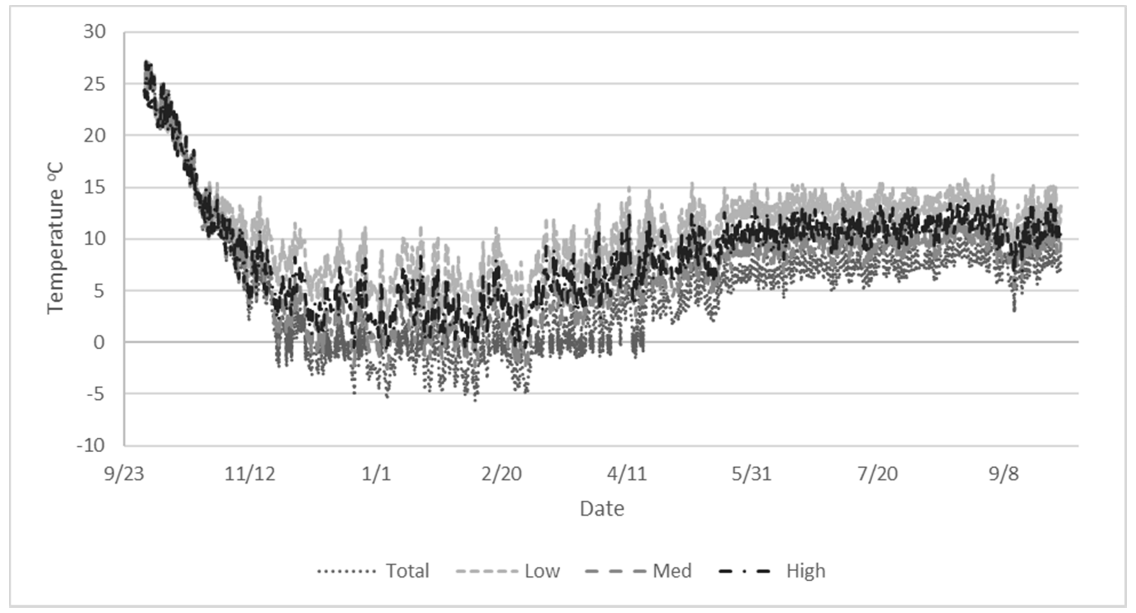
Figure 3 and
Figure 4 show the average temperatures over time predicted for the sensors of the three cable configurations for the one-year aerated storage period. It is important to note that the predicted values are for the same aeration simulation (i.e., fan controlled based on the temperature of the center cable mid-point sensor), and that the observed differences are due to the difference in the number and placement of the sensors within the grain mass. For the low sensor distribution (i.e., one temperature cable in the center), the overall average temperature for the one-year period was −5.3 °C (8.56 °C SD). For the medium sensor distribution, the one-year average temperature was −0.6 °C (7.84 °C SD), and for the high sensor distribution, it was −1.3 °C (8.01 °C SD). The average temperature for the numerical solution that takes into account all 2940 nodes was 6.1 °C (5.34 °C SD).
As is evident in the figures, the medium and high sensor distributions had similar results for most of the simulated period. The low sensor distribution shows a similar pattern but reported average temperature is consistently cooler throughout the year. The pattern for the average temperature of the numerical solution (“total”) shows much larger daily variability due to the grain temperature in the periphery as influenced by the daily weather pattern. As a result, the numerical solution showed consistently warmer temperatures than the three cable configurations ranging from 5–10 °C for the medium and high sensor distributions and 7.5–12.5 °C for the low sensor distribution during the January through September storage period.
In order to further compare the predicted temperature patterns and mitigate periphery and center effects, the high sensor distribution results were recalculated by eliminating the center cable sensors (
Table 1). This increased the average temperature by 0.64 °C and resulted in close to the same average temperature as for the medium sensor distribution. During the winter months (December–February), the medium sensor distribution, with sensors 1/3 of the way from the center, had comparatively warmer values than those 2/3 of the way towards the wall. During spring (March–May), the sensors closer to the wall began to warm earlier, and the trend reversed, with the high sensor distribution less center cable configuration reporting warmer values than the medium sensor distribution. The break-even point occurred in mid-May. When the temperatures of the medium and modified high sensor densities were combined, the average temperature of −0.67 °C was essentially the same as the high sensor distribution less center cable configuration.
In order to understand the size of the periphery effect, data reported from only one temperature cable near the silo wall was considered. A cable 0.52 m from the wall (6.78 m from the center) reported an overall average temperature of 17.6 °C, a cable at 0.82 m from the wall reported 21.8 °C, and a cable at 1.0 m reported 22.0 °C, and a cable at 1.15 m reported 19.5 °C. This result indicates that after the first meter, temperatures begin to drop and the periphery effect is minimized. The higher temperatures in the periphery are somewhat offset by temperatures near the wall during the cold winter period. However, it appears that highly elevated average temperatures persist for the first 1 m into the grain mass from the sidewall. This result is significant, as more than 25% of the volume in this silo is within 1 m of the wall.
The above simulation results did not take into account how a stored grain manager may make decisions based on all temperature data available to turn on and off aeration fans. In
Figure 5 and
Figure 6, results are shown for aeration fans turned on whenever ambient air is cooler than the average of the sensors for a given cable configuration, and the average of those sensors was above 0 °C.
Figure 5 shows average temperatures during the one-year aerated storage period as the stored grain manager would see them reported by the sensors of the three cable configurations and used by the controller to turn on and off aeration fans. As can be seen, there was little difference in what the stored grain manager would see in terms of average temperatures. The average temperatures over the one-year aerated storage period were 3.6 °C, 3.7 °C, and 4.1 °C for the low, medium, and high sensor distributions, respectively. Most of the observed differences occurred during the initial fall cooling period (October through mid-November). Once the grain mass reached around 0 °C, a stored grain manager would observe little difference between the average grain temperatures. However, the sensors used here do not reveal the whole story, and the stored grain manager should not conclude that number and placement of temperature sensors do not matter when deciding to turn on or off aeration fans to maintain grain quality.
Figure 6 shows average temperatures calculated for the entire grain mass based on the aeration simulation results of the three cable configurations. As can be seen, the results show much warmer temperatures overall when compared to the results showing only sensor values, because they include the highly variable periphery values. The average temperatures over the one-year aerated storage period were 10.8 °C, 7.2 °C, 8.5 °C, 10.7 °C, and 8.5 °C for the low, medium, high, and modified high and high plus medium sensor distributions, respectively, and 4.9 °C for the numerical solution.
The trends for each cable configuration and the numerical solution for all nodes over the one-year storage period were consistent, as demonstrated in
Table 2. The numerical solution resulted in the coolest grain, with an overall average temperature 2.3 °C lower than the medium sensor distribution, which resulted in the coolest grain among the cable configurations tested. The medium sensor distribution resulted in slightly lower temperatures (by 1.25 °C) than the high and modified sensor distributions despite employing fewer sensors (18 vs. 36, 42 and 54). With the center cable removed, the modified high sensor distribution resulted in warmer grain on average than the medium case (by 3.45 °C), and even warmer than the original high sensor distribution (by 2.2 °C). The medium plus modified high sensor distribution resulted in grain with an average grain temperature equal to the high sensor distribution over the one-year storage and with the same variability. In comparison, the medium sensor distribution with fewer cables (and sensors) resulted in a larger variability, with the highest standard deviation of any of the sensor cable simulations except for the numerical solution. The low sensor distribution resulted in the highest average temperature and least variability, which was primarily caused by the core of the grain mass cooling relatively quickly in October and not being further affected by the rewarming of the periphery grain during non-fan operating periods.
In order to compare the results for a conventional temperature cable system to those of a new system using wireless technology, the same aeration strategy was used with 10 replicates for randomizing horizontal sensor locations. The results are shown in
Table 3. A similar trend was seen for the overall average temperatures. The low number of sensors resulted in slightly warmer grain, and the medium number of sensors in slightly cooler grain. The average temperature values were within 0.11 °C for the three sensor distributions likely due to the averaging effect of ten replicates each. The standard deviations and the largest differences (between the maximum and minimum average temperatures) observed between the ten replicates show a clear improvement in the reliability of results as more sensors are included to make aeration decisions. The standard deviation decreased from 0.61 °C for the low number of sensors (one randomly located sensor at each sensor depth) to 0.40 °C for the medium number of sensors (three sensors randomly located at each sensor depth) to 0.33 °C for the high number of sensors (seven sensors randomly located at each sensor depth), i.e., almost by half. Similarly, the average difference between the maximum and minimum average temperature values reduced almost by half. However, fewer cables (and sensors) that result in acceptable stored grain conditions would reduce fixed and variable costs for stored gain managers, and would thus favor randomly placed wireless over fixed-placed cable sensors. The fan-run hours were similar for the three sensor distributions, and less variable with more sensors. They were consistent with those for the medium and high distribution of fixed-placed sensors and resulted in 30% fan run time during the 5-month cool-down and winter holding period.
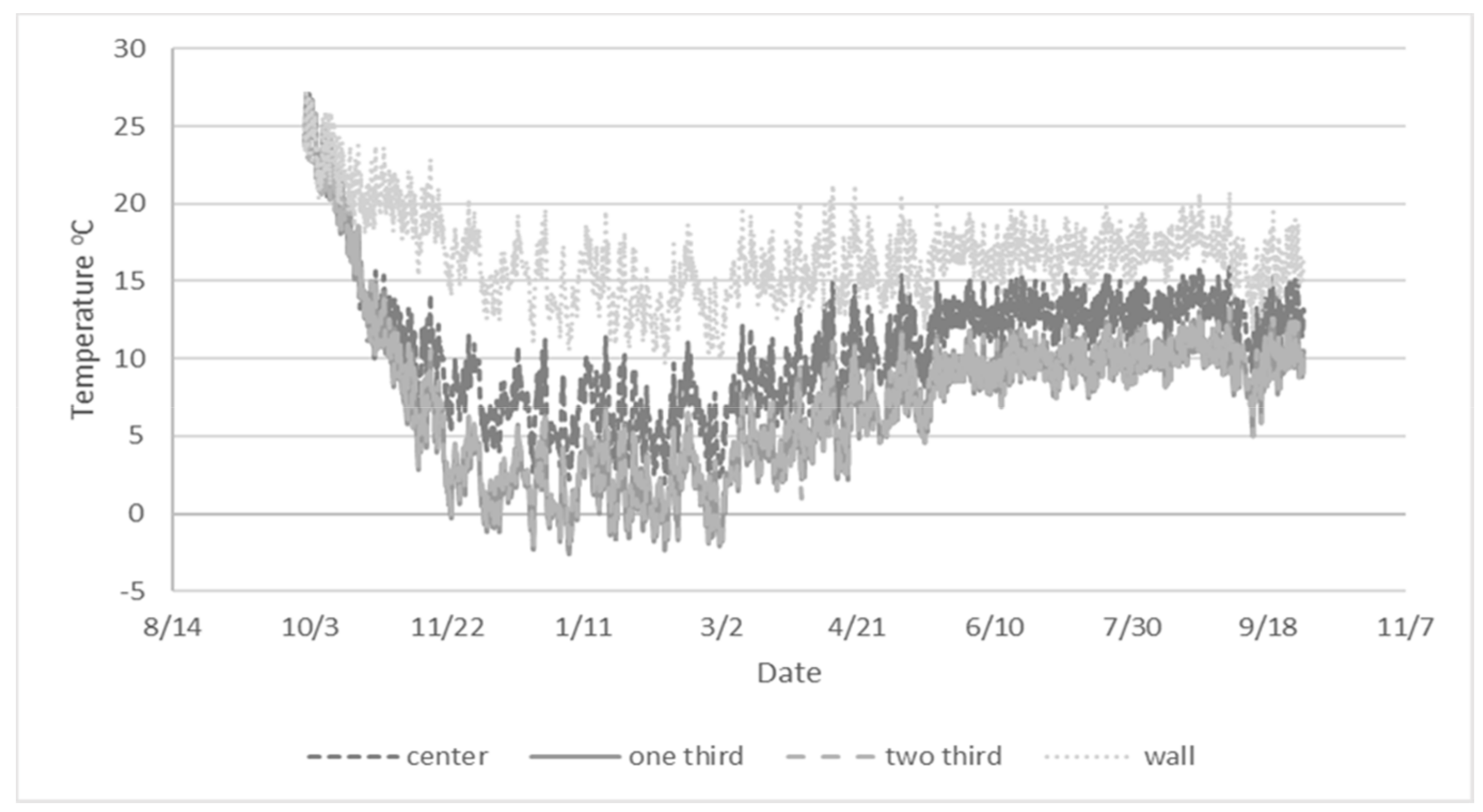
In the final analysis, the effectiveness of aeration cooling was evaluated by turning aeration fans on and off based on the average temperature of six sensors on a single cable placed at four different locations in the grain mass. The single temperature cable located at the wall resulted in the warmest grain mass as the average temperature of all 2940 nodes remained above 15 °C until 21 March (
Figure 7). The sensors in the periphery reported cool conditions during the winter resulting in no need for additional aeration despite the grain bulk remaining warmer.
When placed in the center, the single temperature cable was the second-worst option, reducing the average grain temperature of the grain mass below 15 °C as fast as the one-third and two-thirds location placements, but maintaining a higher average temperature for the remainder of the storage period. The average temperature of the grain mass when the single temperature cable was placed one-third of the distance to the silo wall was about the same (within 0.08 °C) as the one placed two-thirds of the way, and the patterns essentially overlapped during the aeration cool-down and storage periods.
The average grain temperatures for the center and periphery simulations were higher (by 3–9 °C) than the previous scenarios, while the 1/3 and 2/3 scenarios were similar. Results were consistent in that neither the center nor the periphery of the grain mass was ideal for placing a single cable as neither location represents the grain volume at-large. Temperature sensors placed about one-third of the way between the regions that are most (periphery) and least (core) affected by weather conditions appear to be the most representative for monitoring grain conditions with a single cable (or set of wireless sensors) for the silo size evaluated. It will result in rapid and maximum cooling of the grain mass during the all-important fall aeration period. The fan-run hours for the center, one-third, two-thirds, and periphery simulations were 741, 1019, 1044, and 889 h, respectively, and consistent with previous results. However, these results need to be further investigated for different silo sizes.
4. Discussion
These results are of importance to stored grain managers because they demonstrate that they essentially have no control in terms of temperature management over the periphery layer of a grain mass. Additionally, temperature values they rely on to make informed aeration control and inventory management decisions heavily depend on the sensor numbers and placement in the rest of the grain mass. Depending on the temperature cable configuration, the average grain temperature reported may be off by several degrees (e.g., 6–12 °C in these examples) from the overall temperature average in the grain mass. A key reason for this discrepancy is the fact that grain temperatures in the periphery are lowest during winter and highest during summer but are generally not captured because of the lack of cables placed near the silo wall. The silo wall (and thus a 1 m layer of grain closest to the wall) experiences the greatest temperature fluctuations during a one-year storage period. This result highlights one of the problems of temperature cables which are fixed in place and generally not close to the wall.
This result also demonstrates that it is important to select the sensors used to decide when fans are turned on and off. In this case, only the center sensor was used to make that control decision. The core of the grain mass is not influenced by the weather effects on the periphery, and once cooled during the all-important fall harvest period, the core remains cooler throughout the remainder of the storage period. This could mislead a stored grain manager into thinking that the grain mass has cooled to a sufficiently low temperature during the fall cool-down phase and is as cool as it could get when the rest of the grain mass is still at a higher temperature and not yet sufficiently cooled to mitigate rewarming of grain during the spring and summer storage phase. As a matter of fact, a 4.7 °C difference in the average temperature was observed between the low and medium sensor distributions even though the actual conditions were identical across all cases. Activating the aeration fans and operating them to achieve the maximum cooling effect is critical for maintaining stored grain quality and avoiding mold spoilage and insect infestation during the storage period. Thus, relying on the center cable alone is not advisable.
Adding more temperature cables (and sensors) did not provide more useful information than was expected to make informed stored grain management decisions except when temperature readings from the cable in the core of the grain mass was eliminated. The high sensor distribution less the center the cable required six cables and 36 sensors while the medium-plus modified high sensor distribution required nine cables and 54 sensors. For this silo size these additional temperature readings did not provide more useful information for controlling the aeration fan and achieving a lower average temperature than the medium sensor distribution, which utilized only three cables and 18 sensors.
An additional consideration is the number of hours that aeration fans are operated by the automatic controller, which affects cost as a result of electricity consumption. The low sensor distribution had the fewest runtime hours operating for about 20% of the time during the 5-month cool-down and winter holding period (i.e., 741 h out of 3624 h) as shown in
Table 2. In comparison, the medium, high, and modified high sensor distributions operated for about 30% of the time, which would be 50% more costly. The modified high plus medium distribution operated the fan for slightly more than a third of the time, and the average temperature of all nodes called for nearly 50% run time which would be 2.5 times costlier than the low sensor distribution. For this U.S. Midwestern Maize Belt location, the recommended fan operating practice consists of three cycles of 150 h during the October through December cool-down period, which results in a fan run time of 20.4% (i.e., 450 h out of 2208 h) [
19]. Interestingly, only the low sensor distribution matched the recommended practice relatively over time. However, by allowing fans to operate whenever ambient air was cooler than the average temperature reported by the sensors and the average was above 0 °C, fans operated 65–264% more hours (and costlier) than would supposedly be needed based on recommended practice. These findings need to be investigated further in order to refine current aeration decision strategies, especially with regard to the progress of aeration fronts through the grain mass from bottom to top and minimizing fan operating hours and associated electricity costs, which are not considered in this analysis.
In terms of temperatures, these results in
Table 3 do not seem to agree closely with those predicted for the three cable-based fixed sensor configurations. For each comparison, the temperature cable results were more than one standard deviation outside the average temperature results for randomized sensor placement. For the low number of sensors case, temperature cable results were more than 4.5 standard deviations (and 2.76 °C) above the average temperature for randomized placement. The medium number of sensors case showed the temperature cables were 1.75 standard deviations (and 0.71 °C) lower than for randomized placement. For the high number of sensors case, temperature cable results were 1.49 standard deviations (and 0.44 °C) above those for randomized placement. The medium distribution case seems to further confirm that excluding sensors placed in the center when deciding whether to turn on or off an aeration fan based on average grain temperature gives the stored grain manager more reliable information to make an aeration control decision than when they are included.
Randomized placement of wireless sensors increases the likelihood that sensors are not placed in the center and that sensors are placed throughout the bulk of the grain mass. This mitigates the core effect by accounting for warmer conditions in the bulk and more variable conditions in the periphery of the grain mass. Randomized placement would result during the filling of a silo assuming wireless sensors are added to the grain stream. Once they hit the grain surface, they will slide or roll at the angle of repose before coming to rest at a location outside the core of the grain mass and sufficient distance away from the silo wall. One disadvantage, however, for not having sensors in the core of the grain mass is that generally stored grain managers do not core the grain mass and remove peaked grain during the harvest season to maximize available storage capacity in a silo. Cooling peaked grain occurs at a much slower rate than the rest of the grain mass due to non-uniform airflow rates. Airflow rates have shown to be almost three times lower through the core of peaked grain than the airflow through the periphery [
20].


