Article

Using Channel and Network Layer Pruning Based on Deep Learning for Real-Time Detection of Ginger Images

1
Shandong Academy of Agricultural Machinery Sciences, Jinan 250100, China
2
College of Mechanical & Electronic Engineering, Shandong Agricultural University, Tai’an 271018, China
3
Shandong Agricultural Equipment Intelligent Engineering Laboratory, Tai’an 271018, China
*
Author to whom correspondence should be addressed.
Agriculture 2021, 11(12), 1190; https://doi.org/10.3390/agriculture11121190
Submission received: 12 October 2021 / Revised: 16 November 2021 / Accepted: 23 November 2021 / Published: 25 November 2021
(This article belongs to the Special Issue Applications of Sensor Technology to Agri-Food Systems)

Abstract

:
Consistent ginger shoot orientation helps to ensure consistent ginger emergence and meet shading requirements. YOLO v3 is used to recognize ginger images in response to the current ginger seeder’s difficulty in meeting the above agronomic problems. However, it is not suitable for direct application on edge computing devices due to its high computational cost. To make the network more compact and to address the problems of low detection accuracy and long inference time, this study proposes an improved YOLO v3 model, in which some redundant channels and network layers are pruned to achieve real-time determination of ginger shoots and seeds. The test results showed that the pruned model reduced its model size by 87.2% and improved the detection speed by 85%. Meanwhile, its mean average precision (mAP) reached 98.0% for ginger shoots and seeds, only 0.1% lower than the model before pruning. Moreover, after deploying the model to the Jetson Nano, the test results showed that its mAP was 97.94%, the recognition accuracy could reach 96.7%, and detection speed could reach 20 frames·s−1. The results showed that the proposed method was feasible for real-time and accurate detection of ginger images, providing a solid foundation for automatic and accurate ginger seeding.

1. Introduction

Ginger is a warmth-loving crop. However, it is susceptible to high temperatures. It is now widely planted in tropical, subtropical, and temperate regions, and China has the highest yield globally [1]. As shown in Figure 1, it is necessary to cut ginger into small pieces before planting and then use it for seeding after accelerating the germination. Generally, there are 1–2 ginger shoots left on each ginger. The adjustment of ginger shoot orientation is a critical part of the ginger sowing, and its planting agronomy requires that the ginger shoots face the same direction and are southwest [2]. This practice is conducive to the accumulation of heat in the young shoots to grow strong seedlings and play a role in shading the newborn seedlings during the main stem grows. Currently, on large farms in Europe and the United States, ginger is planted mechanically without regard to the orientation of the ginger shoots. However, planting is mainly done in small plots by manual work in China, and ginger seeds should be placed flat in the planting ditch according to the requirements of keeping the ginger shoots orientation consistent during sowing. The development of the ginger industry is seriously hampered by many factors, such as high labor intensity and low efficiency in the manual sowing process. Existing ginger seeders cannot automatically adjust the orientation of ginger shoot to meet the consistency of its orientation, so they cannot be popularized on a large scale. The rapid identification of ginger shoots and seeds through edge computing devices (ECD) are essential to promote the automation of ginger sowing machines and improve ginger yield and the economic efficiency of ginger farmers.
In recent years, with the rapid development of deep learning technology, object detection has been widely used in the biosystems engineering domain [2,3,4,5,6,7]. It overcomes the insufficient representation capability of traditional machine vision and automatically extracts image feature information by building deep convolutional neural networks (CNN) [8]. For example, Xiong et al. [9] adopted the YOLO v2 (you only look once v2) network to estimate the number of mangos. Moreover, YOLO v3 had been widely used for the recognition of lychee fruits and stems [10], weeds [11], tea shoots [12], coffee fruits [13], and cows [14,15,16]. The above findings showed that the YOLO [17,18,19] series network had achieved good results when processing images in the biosystems engineering domain, which reduces manual pre-processing and post-processing steps. However, the computational cost of the model was significant, and it is hard to apply the model onto the ECD with limited functions. Therefore, our goal was to make the network more compact for automatic ginger seeding using the ECD [20]. The common methods of network thinning are classified into the following four types according to the pruning object: fine-grained pruning [21], vector-level pruning [22], kernel-level pruning [23], and filter pruning [24,25]. Among them, the first three approaches strike a balance between the number of parameters and the model performance, but the network’s topology is changed, requiring a specific network framework or even specialized hardware support, and it is known as unstructured pruning. The last approach only changes the number of filters and feature channels and does not require a specific framework and hardware support, so it is called structured pruning [26]. The above research on the basic theory of pruning provides a reference for the application of pruning. In the field of agriculture, many scholars have proposed different methods for different networks in order to achieve network slimming [27], including network pruning [28], knowledge distillation [29], and model quantification [30], among which network pruning is a simple and effective compression method [31], which can obtain a pruned model simply by trimming the number of channels and network layers.
By adding constraints to the channels and evaluating their importance during network training, it is possible to remove some non-critical channels without significant performance degradation. In ginger recognition, to address the problems of low detection accuracy and long inference time, and effectively compress the model size, this work proposes a YOLO v3-based channel and network layer pruning method to detect ginger images in real-time. Firstly, this method uses a comprehensive and sizeable YOLO v3 model as the input model, and after fine-tuning the model, ginger detection is achieved. On this basis, channel pruning, and network layer pruning algorithms are used to prune the trained model, and the structure and parameters of the model are simplified with guaranteed accuracy, resulting in a thin and compact model. The above research provides a solid foundation for deploying the model to the ECD and ginger’s automatic and accurate seeding. In future field experiments, we try to install the imaging system on the ginger seed delivery channel of the planter for real-time image acquisition and deploy the model to the ECD for ginger grasping and ginger shoot direction adjustment using an end-effector device. The rest of the paper is organized as follows: Section 1 presents the creation of the dataset and the channel and network layer pruning model based on the YOLO v3 network; Section 2 describes the tuning of the model parameters and the experimental validation of the proposed method; Section 3 discusses transfer learning, the shape of the bounding box, the causes of incorrect identification, and the practical requirements of the model; Section 4 describes the conclusions.

2. Materials and Methods

2.1. Image Acquisition System

In this study, “Baby Ginger” from Anqiu, Shandong, China, is chosen as the experimental subject with ginger shoots of 0.5–2.0 cm in length. The ginger images are taken from 20 to 27 April 2020, and the acquisition method is shown in Figure 2, and the imaging device included studio (1), CMOS (complementary metal oxide semiconductor) industrial camera (2), computer (3), fill light (4), and camera stand (5). The camera model is the Hikvision MV-CE200-10GC with a zoom lens, and the shooting distance is 25 cm. A total of 1400 images with a resolution of 5472 (horizontal) × 3672 (vertical) pixels are collected and saved in a “JPG” file format. The ginger images obtained by the imaging device are of high resolution, so the images are scaled to 416 × 416 pixels to reduce training time and memory usage by using bi-cubic linear interpolation. The specific process is as follows: the short edge is scaled by the same multiple after scaling the long edge to 416 pixels to prevent image distortion, and then the image is filled to 416 × 416 pixels using grey pixel dots [32]. In addition, as shown in Figure 2, this work uses the LabelImg (https://github.com/tzutalin/labelImg, accessed on 15 March 2021) plugin to label and annotate the ginger shoots and seeds in xml standard format to determine the orientation of the ginger shoots and ensures that the label box is tightly close to the target edge.
Before model training, the dataset is randomly divided into training, validation, and test (A) sets in the ratio of 70%, 20%, and 10%, with no duplication among each other. Meanwhile, this study uses data augmentation [33] to enrich the ginger dataset and improve the model generalization capability. Data enhancement methods include horizontal flip, vertical flip, mirror flip, adjustments to hue, saturation, brightness, image resizing, and adding Gaussian noise. Moreover, the test (B) set is obtained after data augmentation.

2.2. Overall Technical Route

As shown in Figure 3, to achieve real-time and accurate detection of ginger seeds and shoots in the model training, the technical solution proposed in this study is as follows: (1) Analysis and pre-processing of ginger images. Firstly, the images are annotated and divided into training, validation, test set. Secondly, the original training and test sets are enhanced to build the ginger dataset for the few ginger images taken. (2) CNN construction and training. This study constructs a ginger recognition network based on YOLO v3 and pre-trains the Darknet-53 model using the ImageNet [34] dataset. Then, its first 74 layers weights are used as the pre-training model to achieve transfer learning [35,36,37]. (3) Ginger recognition model optimization and pruning. This study obtains a model with excellent performance after continuously adjusting the learning rate, which means the model has a high mAP and faster detection speed to complete the basic training. Then, many redundant channels and network layers are pruned to reduce the model parameters, thus reducing the model parameters. (4) Model performance analysis and testing. This work analyses the number of channels and network layers pruning and verifies its performance using YOLO v3 for different backbone networks and YOLO v4. Finally, the pruned model is deployed onto an ECD for testing.

2.3. Network Structure for Ginger Recognition Based on YOLO v3

YOLO v3 is a new object detection algorithm proposed on the basis of YOLO v2. It uses the Darknet53 network, an idea based on residual learning. Compared to two-stage object detection networks, it transforms the detection problem into a regression problem, and it can directly regress to generate classification results and positions of the objects through the CNN, which significantly improves the detection speed. YOLO v3 works as follows: firstly, the input image is divided into S × S grid cells, each grid includes three a priori boxes, consisting of bounding box coordinates, confidence, and category, respectively. The anchor box is then used as the a priori bounding box to impose constraints on the prediction bounding box and is detected in each grid cell. Finally, the bounding box of the target is located using an independent logistic regression classifier.
As shown in Table 1, the overall structure of the ginger recognition network consists mainly of a series of 1 × 1 convolution and 3 × 3 convolution, with 107 layers in total. On the one hand, the first 74 layers of the network are a Darknet-53 network, without a fully connected layer (FC), for extracting ginger features, including n-CBL (convolution, batch normalization, Leaky-ReLU) modules and n-RES (Resnet) modules. Among them, the n-CBL module consists of n CBL modules, where the CBL module is composed of a convolution (Conv) layer, a batch normalization (BN) layer, and a Leaky-ReLU activation layer in turn; and the n-RES module consists of CBL module and n residual blocks that draws from the ResNet network and uses Shortcut connections to form a deeper network.
On the other hand, the last 33 layers of the ginger recognition network are the multi-scale feature fusion layer and the output layer, including the n-CBL module, the Route layer, the up-sample layer, and the YOLO layer. Among them, the Route network layer splices the deep feature map with the shallow feature map to improve model generalization capability by increasing the tensor dimension and fusing the features extracted from different network layers; and the up-sample layer deepens the network by implementing up-sampling on the feature maps; and the YOLO layer completes the classification and location regression of ginger shoots and ginger seeds.
Although YOLO v3 enables the detection of ginger, the number of parameters and structure of YOLO v3 is large, resulting in a large number of calculations. To reduce the complexity and parameters of the model and facilitate its application onto the ECD, the model needs to be pruned.

2.4. Sparse Training Based on Channel Importance Evaluation

In the ginger recognition network, the BN layer is located after the Conv layer and before the Leaky-ReLU activation layer and accelerates the training speed and prevents the gradient from disappearing or exploding by normalizing the output value of the Conv layer. The calculation formula of the BN layer is as follows:
y = γ · x E [ x ] V a r [ x ] + ε + β
where γ and β are neuron conditioning parameters for scaling and translating the normalized neurons to enhance the network expressive power and obtained through network training; and x is the output channel of the Conv layer, and y is the output of the BN layer; and E[·] and Var[·] are the mean and variance of x; and ε = 1 × 10⁻⁶ is to prevent the denominator from being 0.
The ginger recognition model contains a large number of redundant channels after basic training, and the number of channels varies significantly among different BN layers, with a minimum of 32 and a maximum of 1024, so this work uses sparse training to solve the pruning problem with significant differences in the number of channels. During sparse training, this study added the L- normalization term for the γ-values in the BN layer to the loss function, making a large number of γ-values converge to 0 during the gradient update. Thus γ-values become sparse. The L1-normalization is easy to eliminate the channels that do not provide helpful information for the final output. The L1-normalization of γ-values for each channel in the BN layer is calculated as follows:
γ 1 = i = 1 n γ i
where |γi| is the absolute value of the γ-value for the ith channel. The objective function of sparse training is as follows:
L oss = ( x , y ) l ( h θ ( x , θ ) , y ) + α γ 1
where the first term is the training loss of the network, x and y are the input and output of the training, respectively; θ is the trainable weight, and hθ is the output value of the forward propagation; l(·)denotes the training loss of the target; ||γ||1 is the L1-normalization of the γ-values; α is a constant coefficient used to tune the optimization objective function.

2.5. Channels and Network Layers Pruning Algorithms

Pruning of ginger recognition networks mainly includes channel pruning and network layer pruning. Channel pruning is essentially an algorithm that eliminates channels with a γ-values of 0 after sparse training, and it does not change the number of channels or the size of the feature map. Furthermore, the channel pruning algorithm reduces the model parameters while maintaining the network structure intact, and it does not require a specific network framework or hardware support, making it more convenient to deploy in mobile devices. Therefore, this study uses the channel pruning algorithm to prune the trained ginger recognition network.
As shown in Figure 4, the channel pruning for the ginger recognition model uses γ-values to evaluate the importance of its channel. Suppose the γ-values are close to 0 (as in the red line), the output of the activation layer is also close to 0, so the channels where the γ-values are located have little effect on the whole network and can be pruned. The redundant channels are pruned as follows: it is first necessary to find the index value of the BN layers to be pruned. Secondly, the absolute values of γ-values are extracted into a list and sorted from the minimum to the maximum value. Finally, a p-value is defined to control the pruning ratio in the BN layer, and a global threshold γ ^ is defined to determine the upper limit of γ-values to be pruned, whose size is the pth percentile of all γ-values in the list. This indicates that when the γ-value of a channel is less than γ ^ , it will be pruned. Thus, γ-value are obtained according to different channel pruning ratios, which enables the pruning of redundant channels. Furthermore, the largest γ-value in each channel is ranked, and its minimum value is used as the upper limit for γ-values pruning to avoid pruning all channels, which ensures the integrity of the network. If γ-values of the pruned channels are equal to 0, the performance of the pruned model is similar to the sparse training model that almost equals the basic training model.
When a channel is pruned, its γ-value is set to 0. Regardless of the output value from the Conv layer before the BN layer, it can be seen from Equation (1) that the output value of the BN layer is β that became β1 after the Leaky-ReLU activation function. The above description showed that the channel still has some influence on the subsequent modules. This study performs the following operations to compensate for the computational bias caused by β-values. (1) When the subsequent module is CBL, E[x] of the BN layer is subtracted by β1. (2) When the subsequent is a Conv layer, the β1 is added to the bias of the Conv layer. (3) When the subsequent is a Shortcut or up-sample layer, the β1 is passed until it meets the CBL or a Conv layer, and operation (1) or (2) is performed.
This study prunes the redundant residual blocks in the ginger feature extraction network after channel pruning. As shown in Figure 5, the residual block consists of two CBL modules and a Shortcut layer, and the features to be learned from the shallow lth layer to the deep Lth layer are as follows:
x l + 1 = h ( x l ) + i = 1 l F ( x i , W i )
where xl and xl+1 are the input and output of the lth residual block, respectively; and h(xl)=xl denotes the identity mapping; and L denotes the number of residual blocks; and F(·) is the residual function that represents the learned residual information; and Wi is the trainable weight of the residual function.
In pruning the redundant residual block, the study first ranks the mean of γ-values in the previous CBL of all Shortcut layers. If it is close to 0, then xl+1 = xl from Equation (4), which means that this residual block has not learned helpful information, then pruning it will not affect the network performance. As a result, the residual block with a smaller mean of γ-values will be pruned.
Since many γ-values converge to 0 after sparse training, the model’s redundant channels and network layers are pruned to reduce the parameters, size, and inference time of the model. However, the model performance decreases due to the pruning of many γ-values that are not equal to 0. Therefore, this study fine-tunes the pruned model to compensate for the decrease in model performance.

2.6. Experimental Devices and Model Testing

During the model training, the workstation configuration was Intel Core I9-9900K CPU 3.6 GHz, 64 GB running memory, 200 GB Solid State Drive, 11 GB Nvidia GTX 2080Ti GPU, CUDA version 10.1 parallel computing architecture, and CUDNN version 7.6 network acceleration library. The running environment was Ubuntu 18.04, Python 3.6.5, and Pytorch1.5.1, Numpy1.18.1, Opencv4.5.3, Tensorboard2.2.2, Scipy1.4.1, Pillow7.1.2. The model optimization method was SGD, the momentum is 0.95, the weight decay coefficient is 5 × 10⁻³, and the batch size was 16. The training strategy was set as follows: In order to obtain nine suitably sized clustering boxes before network training, the width and height of the labeled boxes in the dataset are clustered by K-means, which adopts an IoU-based distance measure with the objective function of minimizing the distance between the labeled boxes and the clustering centers, and ultimately, 9 clustering boxes are obtained, and the sizes are (24, 25), (33, 44), (41, 57), (49, 75), (212, 175), (280, 195), (236, 248), (308, 246), and (352, 342), which were applied to initialize the anchor boxes in the ginger recognition network. Besides, this study introduces the Distance Intersection over Union [38] bounding box regression loss function to improve the regression effect of the predicted box.
In the initial stage of network training, this paper proposed a new learning rate warm-up strategy to make the network converge to a better initial state, which uses 20 epochs to linearly increase the learning rate from 1 × 10⁻⁶ to 1 × 10⁻², and then adopts the conventional learning rate adjustment strategy to decay it to 1 × 10⁻³ and 1 × 10⁻⁴ at the stage of 0.7 and 0.9 of the total training epochs, respectively. This method allows the learning rate to gradually increase from small to large so that the model can reach a better initialization state. Furthermore, this study uses the training set to train single-stage object detection networks to validate the model performance, such as YOLO v3 with different backbone networks and YOLO v4, respectively. Then, the performance of the various detection networks is evaluated using ginger images from the test set to validate the advantages of the proposed pruning algorithm.

2.7. Performance Evaluation Metrics

The paper uses five metrics, Precision(P), Recall(R), F1-score, mean average precision (mAP), and detection speed, to evaluate the model performance. the calculation formula is as follows:
P r e c i s i o n = T P T P + F P × 100 %
R e c a l l = T P T P + F N × 100 %
F 1 - s c o r e = 2 P × R P + R × 100 %
m A P = 1 m A P = 1 m 0 1 P ( R ) d R × 100 %
where TP, FP, and FN are the number of true positives, false positives and false negatives respectively. m is the number to be classified, there are two categories, ginger shoots and seeds, in this study, so m = 2. When the model is tested, P, R, and F1-score cannot be used as constant model properties because they can be changed by adjusting the confidence threshold according to different task requirements. However, mAP, as the mean value of different classes of AP that is the mean value of all P with different R, can be used as a constant model property. Therefore, mAP can be used as the primary performance evaluation criterion [39] in this paper. The detection speed includes the recognition speed of a single ginger image on a high-performance computer and Jetson Nano device.

3. Results

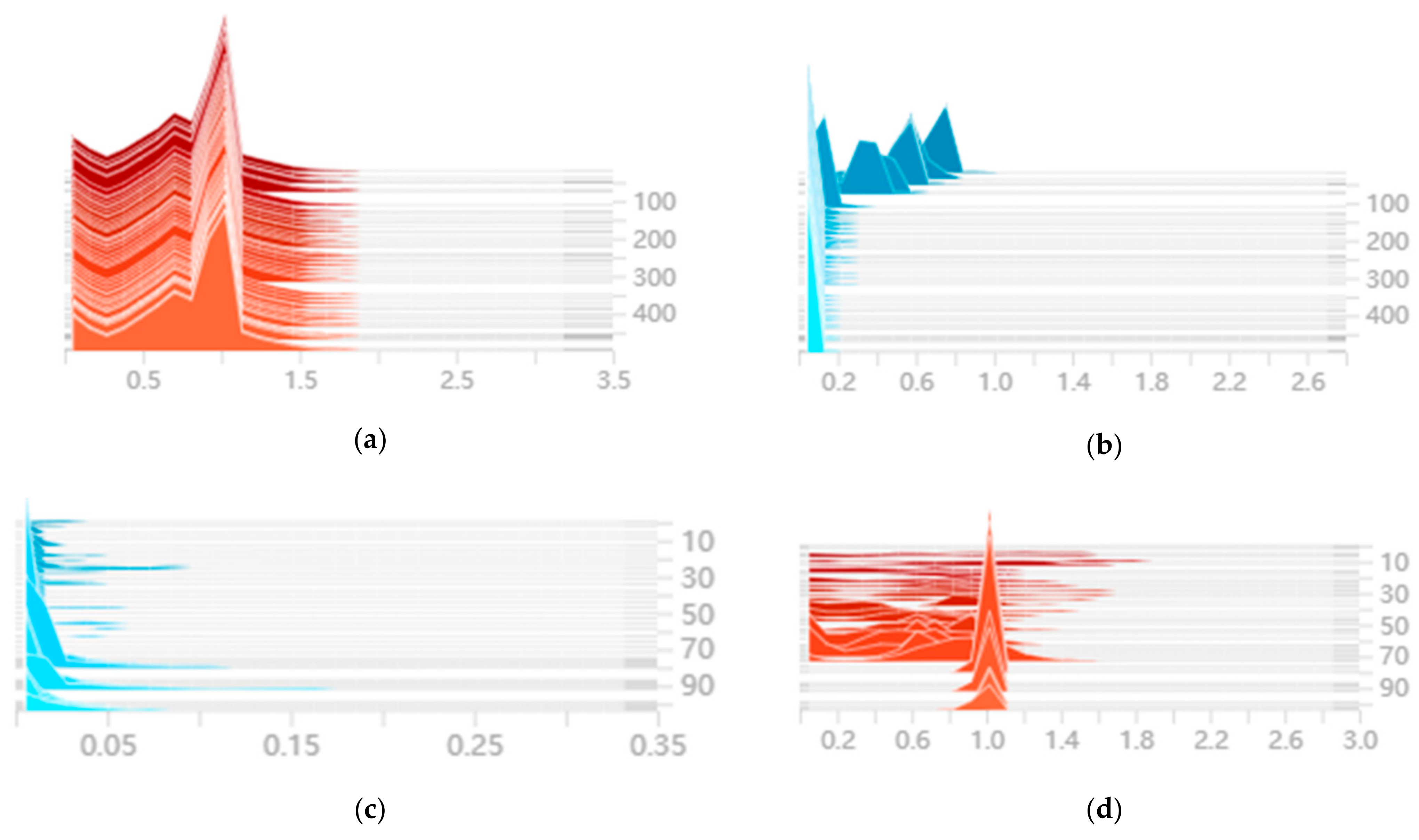
3.1. Parameter Selection for Sparse Training

The sparse training was achieved by adding the L1-normalization of γ-values for the BN layer into the loss function of the ginger recognition network, and the constant-coefficient α in the loss function was set to 5 × 10⁻⁴, 1 × 10⁻³, 5 × 10⁻³, respectively, to maintain high performance and high sparsity of the sparse model. As shown in Figure 6, when α was 1 × 10⁻³ after sparse training of 500 epochs, the ginger recognition network had a faster convergence speed, a better convergence effect.
During the sparse training, the γ-values and their frequencies of occurrence were recorded using the Histograms function in the Tensor-board module in real-time. Figure 7 shows the distribution of the scaling factor γ-values in the BN layer, where the x-axis indicates the distribution of γ-values, the y-axis in Figure 7a,b displays the training epochs, and the other y-axis shows the number of network layers. As shown in Figure 7a, after basic training of 500 epochs, the distribution of γ-values for the BN layer was close to a normal distribution with a mean value of 1. As shown in Figure 7b, after sparse training of 500 epochs, the mode of the γ-values for the BN layer decreased from the initial 0.753 to 0.0442, gradually approaching 0, but not all values decayed to 0. Furthermore, the sparsity of γ-values remained unchanged when epochs were 200, so reducing α to the original 100 times would help the model performance rebound. As shown in Figure 7c,d, the distribution of γ-values for each network layer before and after sparse training is shown, respectively, and the sparse training compressed γ-values of channels with lower importance to near 0, which was convenient for later pruning operations.

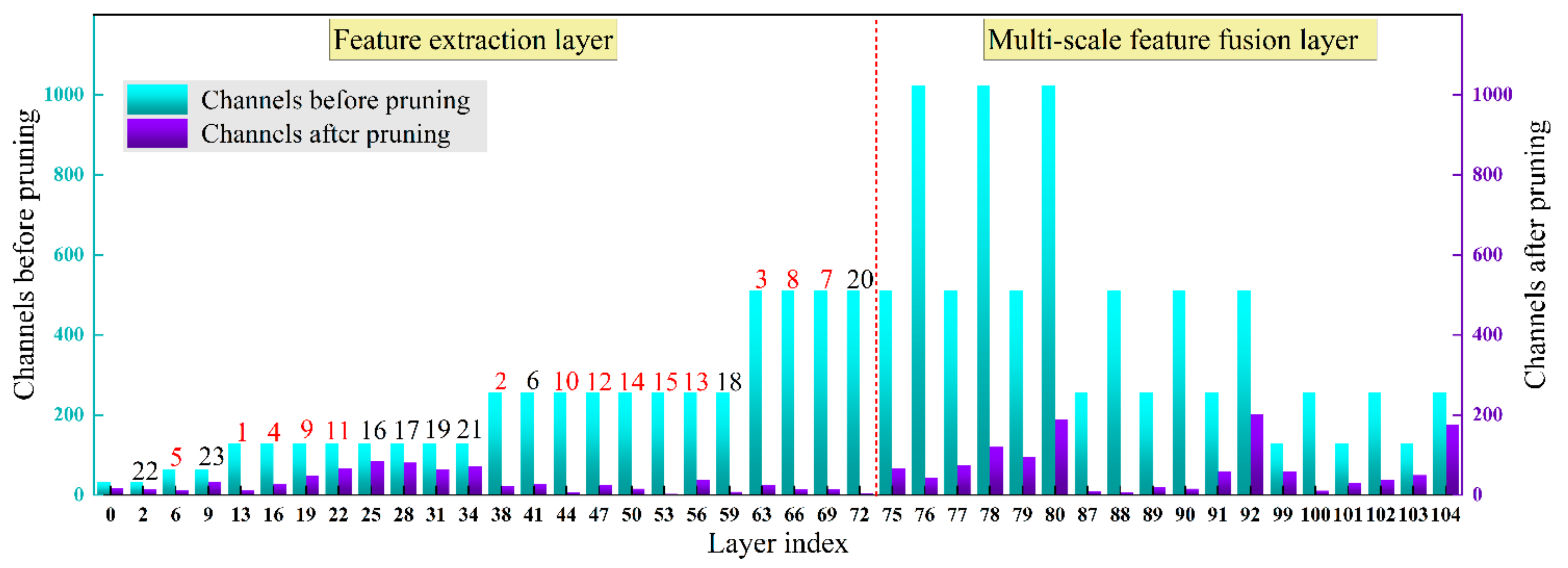
3.2. Parameter Selection for Pruning Process

The tradeoff curve of mAP and the number of parameters during pruning are shown in Figure 8, where the lower x-axis is the channel pruning rate, and the upper x-axis is the number of layers pruned, and four trade-off curves are obtained for direct channel pruning (purple dashed line), channel pruning + fine-tuning (solid green line), direct network layer pruning (yellow dashed line), and network layer pruning + fine-tuning (solid red line), respectively. It is commonly said that the more parameters were pruned within a specific range, the lower the model performance. Comparing the solid and dashed lines in Figure 8 shows that the role of fine-tuning was crucial. On the other hand, comparing the purple dashed line and the solid green line, when the channel pruning rate was less than or equal to 60%, the mAP was almost constant, and the number of parameters was reduced by 0.26 times without fine-tuning. When the channel pruning rate was greater than 70%, the mAP dropped rapidly to 0 without fine-tuning due to the pruning of many γ-values that were not truly equal to 0. Thus, the pruned model was fine-tuned by 200 epochs to recover the model performance. When the pruning rate was 85%, the fine-tuned model still maintained a high mAP of 98%. Moreover, comparing the yellow dashed line with the solid red line, the mAP gradually decreased as the number of residual blocks in the backbone network decreased when directly pruning the network layers. However, the performance of the fine-tuned model remained unchanged at less than 45 network layers, and mAP was stall around 98%.
The changes in the number of channels and network layers in the BN layer after model pruning are shown in Figure 9. The number of channels in each BN layer was significantly reduced in both the feature extraction and multi-scale feature fusion layers, with the total number reduced from 13,376 to 279. There were 23 residual blocks in the feature extraction layers, and a total of 69 network layers could be pruned. In the model with a channel pruning rate of 85%, the residual blocks were pruned sequentially according to the mean absolute value of the γ-values in the BN layer. As shown in the numbers above the bars chart in Figure 9, where the larger the number, the more critical the residual block where the BN layer was located. The red numbers represented the pruned residual blocks, and the number of network layers was reduced from 107 to 62 after pruning.

3.3. Analysis of mAP Curves during the Training of a Ginger Recognition Mode

The variation of the mAP curve with epochs during the acquisition of the ginger recognition model is shown in Figure 10, where the first 500 epochs is the basic training, 500–1000 epochs are sparse training, 1000 epochs is model pruning, and 1000–1200 epochs are model fine-tuning, and plots a, b, c, and d, respectively, show the distribution of γ-values at the above four stages, and the red curves are the normal distribution curve of γ-values. It can be seen from Figure 10 that the mAP curve stabilized after basic training of about 400 epochs, and the final mAP value was 98.1%. The total number of γ-values was 13,376 at this time, and their mean value was 0.907, the minimum value was 0.086, and the maximum value was 2.897. In the first 350 epochs of the sparse training stage, the gradient update of γ-values during backpropagation made a large number of γ-values converge to 0, which led to a sharp fluctuation of the mAP curve. After sparse training of about 350 epochs, the curve tended to stabilize, and the final mAP still remained at 98.0%. As shown in Figure 10b, the total number of γ-values was 13376, most of which were distributed between 0 and 0.1, with a minimum value of 0 and a maximum value of 1.167. As shown in Figure 10c, when the pruning rate was 85%, all γ-values less than 0.072 were set to 0, which resulted in the mAP of 0.0% as many channels with non-0 γ-values were pruned. The model performance was recovered, and mAP reached 98.0% after fine-tuning. As shown in Figure 10d, the distribution of γ-values approximated a normal distribution, with a mean value of 0.298, a minimum value of 0.001, and a maximum value of 1.177.

3.4. Parameter Selection for Sparse Training

The feature visualization of the ginger recognition network from shallow to deep layers helped to understand the recognition process, and the Jet color bars were used to reflect the importance of the features, with image features becoming more critical as the color transitions from blue to red. Figure 11a shows the mapping of the output features from the first convolutional layer of the pruned model, where the size of the feature map is 416 × 416 pixels, and their number is 18. It can be seen from the 18 feature maps that the convolution operation had an excellent smoothing filtering effect and maps the input image to different gray spaces, which effectively improves the anti-interference ability of the network under different lighting conditions. Moreover, the model effectively extracted the underlying features such as contours, textures, and edges.
As the network layers deepened, the output feature maps became more abstract, and the deep semantic information became more prosperous, which provides a better understanding of what the network focuses on. Figure 11b shows the output feature maps of the final YOLO layer, where there are 21 feature maps whose sizes are 52 × 52 pixels. After decoding the feature information of the network using the YOLO layer, it was found that the color of the ginger shoots and seeds were closer to red than other pixels, which indicated that the network had extracted their deeper features well, thus realizing their classification and location regression.

3.5. Comparison of Different Object Detection Algorithms

To verify the superiority of the proposed pruning method, six object detection algorithms were compared in this study, including YOLO v3 from different backbone networks (ShuffleNetv2 [40], MobileNetv3 [41], Ghost-Net [42], Darknet-19 [43], Darknet-53), and YOLO v4. The above six algorithms were trained with ginger recognition models using training and validation sets, respectively, and then the performance of different detection algorithms was evaluated using test sets.
As shown in Table 2, the test results showed that the mAP of the pruned model was only 0.1% lower than the original model, but it was higher than the other five algorithms and reached the detection speed of 185 frames·s−1 for a single image. In addition, the pruned model size was 12.2 MB larger than YOLO v3 with ShuffleNet-v2 as the backbone network, but the mAP was 2.4% higher. Compared with the YOLO v3 with MobileNet-v3, Ghost-Net and Darknet-19 as the backbone networks, and the YOLO v4, the pruned model outperformed them in terms of both mAP and model size. The above results showed that the mAP of the pruned YOLO v3 model was 98.0%, including the AP of 97.4% for ginger shoots and 98.6% for ginger seeds. Meanwhile, the pruned model was tested using the enhanced test set B, and its mAP and F1-score reached 97.2% and 93.8%, respectively, indicating that the pruned model had high noise immunity and robustness. With the acceleration of the Tensor RT inference optimizer, the mAP of the pruned model on the Jetson Nano device remained essentially unchanged, and the detection speed could reach 20 frames·s−1, which could perform the ginger detection task well.

4. Discussion

4.1. Analyzing Pre-Trained Network and the Shape of the Bounding Box

The ImageNet dataset has been widely used for transfer learning because it has enough images to help train pervasive models. In addition, these pre-trained networks show good generalization performance for pictures outside the ImageNet dataset. Therefore, this work takes the first 74 layers weights of the DarkNet-53 model trained on the ImageNet dataset as a pre-trained model to extract the feature of ginger shoots and ginger seeds in ginger images. Furthermore, suppose the similarity between the original job of the network and the new task is low according to Yosinski et al. [44]. In that case, the transfer learning will be less effective. The ImageNet dataset mainly consists of everyday items, such as flowers, animals, and plants, which are very different from ginger images. However, the experimental results show that transfer learning achieves good results, and mAP increases by 0.7% compared to training from scratch.
The traditional rectangular bounding box [45,46] is usually used for general object detection tasks to localize the target. In this study, since the detection targets are ginger shoots and ginger seeds, which have very irregular shapes, this work uses conventional rectangular bounding boxes to locate them. Moreover, this study retains only the largest prediction boxes for ginger with multiple ginger shoots and then determines the orientation of the ginger shoots by calculating the relative positions of the two types of prediction boxes, which can be achieved by a rectangular enclosing box.

4.2. Analyzing False Recognition Results

During the detection process of the ginger recognition model, there are many disturbing cases, and this study further improves the performance of the pruned model by analyzing the incorrect recognition results. As shown in Figure 12, the arrows point to the wrong identification boxes, and the reasons for misidentification at arrows 1–4 are as follows: the ginger produces some protrusions that resemble the shape of ginger shoots during germination, but they do not form true ginger shoots, so they are misidentified. The reasons at arrows 5–7 are as follows: the uneven illumination. Therefore, to further improve the model performance, it is necessary to ensure uniform and stable illumination, increase the number of samples, establish the dataset of difficult samples, and continue training the model.

4.3. Analysis of Practical Work Requirements

In model testing using an ECD, the inference of the model was implemented using Jetson Nano. The Jetson Nano is equipped with a quad-core 64-bit ARM CPU, a 128-core NVIDIA Maxwell @ 921MHz GPU delivering 472 GFLOPS (giga floating point operations per second), and includes 4 GB of LPDDR4 running memory. The Jetson Nano uses a 10 W power supply model with a 5V(volt) and 4A (ampere) DC (Direct Current) power supply for the experiments. The running environment is Ubuntu 18.04, CUDA Toolkit 10.0, cuDNN7.3, Python 3.6, Pytorch1.4, opencv3.3.1, Tensor RT (real time) 6.0. Tensor RT is a low latency, high-throughput inference optimizer for deep learning from NVIDIA [47]. It optimizes the network by combining network layers and optimizing kernel selection to reduce latency, throughput, energy efficiency, and memory consumption. What is more, this study first converts the pruned model into an open neural network exchange (ONNX) [48] model to speed up the model inference and then converts it into a Tensor RT inference engine. In addition, this study converts the model to floating-point 16 (FP16) to further speed up the model inference due to the Jetson Nano supporting FP16 inference. Finally, the detection speed of the model on a single ginger image is tested.
In this paper, we analyze the cultivation agronomy of ginger and the technical standards of the ginger seeder developed by us to verify whether the detection speed can meet the seeding requirements. It is understood that the plant spacing of ginger is generally 0.25 m, and the row spacing is 0.5 m. In addition, the seeder’s operating efficiency is 0.05–0.10 hm2·h−1, the rate of ginger shoots facing the same direction is more than 90%, and two rows can be sown at the same time. The formula for seeder efficiency is as follows:
η = 0.36 w h n t
where η is the sowing efficiency, w is the plant spacing (m), h is the row spacing (m), n is the number of rows, and t is the sowing time (s). After calculating Equation (9), the sowing time t is 0.9–1.8 s for single ginger. The test results using the Jetson Nano device show that the accuracy reaches 96.7%, and detection speed reaches 20 frames·s−1, and we can know that the pruned model can meet the working requirements of the seeder through the above analysis.
Due to the irregular shape of ginger and the fragile ginger shoots, we are designing ginger conveying channel and placing an imaging system on top of the channel. During operation, the ginger is manually placed at one end of the channel, and then the end-effector device is used to grasp the ginger and reorient the ginger shoots. In addition, this study will collect more field-captured ginger images in the future and use the current model as a pre-training model to continue optimizing the model.

5. Conclusions

To deploy a ginger recognition model on edge computing devices, this study proposes a channel and network layer pruning algorithm based on YOLO v3 to realize real-time and accurate detection of ginger shoots and seeds. The main findings are as follows:
  • Firstly, the ginger dataset is established, including image acquisition, data enhancement, and image annotation. Next, transfer learning and learning rate warm-up strategies are adopted to identify ginger shoots and seeds accurately. The experimental results reveal that the mAP and F1-score reach 98.1% and 95.4%, respectively, providing a reliable model compression basis.
  • This study prunes the ginger recognition model’s redundant channels and network layers to reduce model parameters and inference time. First, the γ-values in the batch normalization layer are used to evaluate the channel importance, and the unimportant channels are pruned to accomplish the channel pruning. Then, the γ-values of the CBL module before the Shortcut layer are taken to evaluate the significance of the residual blocks, and the insignificant residual blocks are pruned to realize the pruning of the network layer.
  • After channel and network layer pruning, the mAP and model size of the ginger recognition model reach 98.0% and 32.7 MB, respectively, which are reduced by 0.1% and 86.03% compared with the pre-pruning model. With the acceleration of the Tensor RT inference optimizer, the detection speed of a single 416 × 416 pixels ginger image on the Jetson Nano device can reach 20 frames·s−1. This study provides technical support for the future implementation of grasping ginger and adjusting the ginger shoot direction using end-effector devices.
  • The detection of ginger images is only the first step in automated ginger seeding. In the future, the use of detection results for ginger grasping and ginger shoot orientation adjustment will be a hot research topic. Furthermore, our proposed pruning algorithm is not only beneficial for ginger detection, but it can also be applied to other crop detection tasks where computational resources are limited. Future work will focus on more efficient pruning methods and the acquisition of more ginger images under real-world operating conditions to further improve the accuracy of ginger detection.

Author Contributions

All authors contributed to the research. Conceptualization, L.F. and Y.W.; methodology, L.F. and Y.W.; software, L.F.; validation, L.F. and Y.L.; formal analysis, L.F. and Y.W.; investigation, L.F., H.G., H.Z., X.W. and J.H.; resources, J.H. and Y.W.; data curation, L.F.; writing—original draft preparation, L.F. and J.H.; writing—review and editing, J.H. and R.X.; visualization, L.F.; supervision, J.H.; project administration, J.H.; funding acquisition, J.H. All authors have read and agreed to the published version of the manuscript.

Funding

This work was supported by the China Agriculture Research System of MOF and MARA (Grant numbers: CARS-24-D-01), the Shandong Agricultural Major Applied Technology Innovation Project (Grant numbers: SD2019NJ004), and the Shandong Modern Agricultural Industry Technology System Vegetable Industry Innovation Team Project (Grant numbers: SDAIT-05).

Data Availability Statement

Not applicable.

Conflicts of Interest

The authors declare no conflict of interest.

References

  1. Wang, L.; Xun, K.; Li, X. Research status on breeding of ginger germplasm resource and prospect. China Veget. 2013, 16, 1–6. [Google Scholar]
  2. Hou, J.L.; Fang, L.F.; Wu, Y.Q.; Li, Y.H.; Xi, R. Rapid recognition and orientation determination of ginger shoots with deep learning. Trans. Chin. Soc. Agric. Eng. 2021, 37, 213–222. [Google Scholar]
  3. Chen, C.-H.; Kung, H.-Y.; Hwang, F.-J. Deep Learning Techniques for Agronomy Applications. Agronomy 2019, 9, 142. [Google Scholar] [CrossRef] [Green Version]
  4. Wang, C.; Xiao, Z. Lychee Surface Defect Detection Based on Deep Convolutional Neural Networks with GAN-Based Data Augmentation. Agronomy 2021, 11, 1500. [Google Scholar] [CrossRef]
  5. Lu, C.-P.; Liaw, J.-J.; Wu, T.-C.; Hung, T.-F. Development of a Mushroom Growth Measurement System Applying Deep Learning for Image Recognition. Agronomy 2019, 9, 32. [Google Scholar] [CrossRef] [Green Version]
  6. Osman, Y.; Dennis, R.; Elgazzar, K. Yield Estimation and Visualization Solution for Precision Agriculture. Sensors 2021, 21, 6657. [Google Scholar] [CrossRef] [PubMed]
  7. Li, Z.B.; Guo, R.H.; Li, M.; Chen, Y.; Li, G.Y. A review of computer vision technologies for plant phenotyping. Comput. Electron. Agric. 2020, 176, 105672. [Google Scholar] [CrossRef]
  8. Zhu, S.; Zhuo, J.; Huang, H.; Li, G. Wheat grain integrity image detection system based on CNN. Trans. Chin. Soc. Agric. Mach. 2020, 51, 36–42. [Google Scholar]
  9. Xiong, J.; Liu, Z.; Chen, S.; Liu, B.; Peng, H. Visual detection of green mangoes by an unmanned aerial vehicle in orchards based on a deep learning method. Biosyst. Eng. 2020, 194, 261–272. [Google Scholar] [CrossRef]
  10. Liang, C.; Xiong, J.; Zheng, Z.; Zhong, Z.; Li, Z. A visual detection method for nighttime litchi fruits and fruiting stems. Comput. Electron. Agric. 2020, 169, 105192. [Google Scholar] [CrossRef]
  11. Ahmad, A.; Saraswat, D.; Aggarwal, V.; Etienne, A.; Hancock, B. Performance of deep learning models for classifying and detecting common weeds in corn and soybean production systems. Comput. Electron. Agric. 2021, 184, 106081. [Google Scholar] [CrossRef]
  12. Yang, H.; Chen, L.; Chen, M.; Ma, Z.; Deng, F.; Li, M. Tender tea shoots recognition and positioning for picking robot using improved YOLO-v3 model. IEEE Access 2019, 7, 180998–181011. [Google Scholar] [CrossRef]
  13. Bazame, H.C.; Molin, J.P.; Althoff, D.; Martello, M. Detection, classification, and mapping of coffee fruits during harvest with computer vision. Comput. Electron. Agric. 2021, 183, 106066. [Google Scholar] [CrossRef]
  14. Hu, H.; Dai, B.; Shen, W.; Wei, X.; Sun, J.; Li, R.; Zhang, Y. Cow identification based on fusion of deep parts Features. Biosyst. Eng. 2020, 192, 245–256. [Google Scholar] [CrossRef]
  15. Shen, W.; Hu, H.; Dai, B.; Wei, X.; Sun, Y. Individual identification of dairy cows based on convolutional neural networks. Multimed. Tools Appl. 2020, 79, 14711–14724. [Google Scholar] [CrossRef]
  16. Wu, D.; Wu, Q.; Yin, X.; Jiang, B.; Song, H. Lameness detection of dairy cows based on the YOLOv3 deep learning algorithm and a relative step size characteristic vector. Biosyst. Eng. 2020, 189, 150–163. [Google Scholar] [CrossRef]
  17. Redmon, J.; Divvala, S.; Girshick, R.; Farhadi, A. You only look once: Unified, real-Time object detection. In Proceedings of the 2016 IEEE Conference on Computer Vision and Pattern Recognition (CVPR), Las Vegas, NV, USA, 27–30 June 2016; pp. 779–788. [Google Scholar]
  18. Kuznetsova, A.; Maleva, T.; Soloviev, V. Using YOLOv3 Algorithm with Pre-and Post-Processing for Apple Detection in Fruit-Harvesting Robot. Agronomy 2020, 10, 1016. [Google Scholar] [CrossRef]
  19. Koirala, A.; Walsh, K.B.; Wang, Z.; Anderson, N. Deep Learning for Mango (Mangifera indica) Panicle Stage Classification. Agronomy 2020, 10, 143. [Google Scholar] [CrossRef] [Green Version]
  20. Qi, C.; Nyalala, I.; Chen, K. Detecting the Early Flowering Stage of Tea Chrysanthemum Using the F-YOLO Model. Agronomy 2021, 11, 834. [Google Scholar] [CrossRef]
  21. Han, S.; Pool, J.; Tran, J.; Dally, W. Learning both weights and connections for efficient neural networks. In Proceedings of the 2015 Twenty-Ninth Conference on Neural Information Processing Systems (NIPS), Montreal, QC, Canada, 7–12 December 2015; pp. 1135–1143. [Google Scholar]
  22. Anwar, S.; Hwang, K.; Sung, W. Structured pruning of deep convolutional neural networks. ACM J. Emerg. Technol. Comput. Syst. 2015, 13, 1–18. [Google Scholar] [CrossRef] [Green Version]
  23. Li, Y.; Iida, M.; Suyama, T.; Suguri, M.; Masuda, R. Implementation of deep-Learning algorithm for obstacle detection and collision avoidance for robotic harvester. Comput. Electron. Agric. 2020, 174, 105499. [Google Scholar] [CrossRef]
  24. Liu, Z.; Li, J.; Shen, Z.; Huang, G.; Yan, S.; Zhang, C. Learning efficient convolutional networks through network slimming. In Proceedings of the 2017 IEEE International Conference on Computer Vision (ICCV), Venice, Italy, 22–29 October 2017; pp. 2755–2763. [Google Scholar]
  25. Prakosa, S.W.; Leu, J.S.; Chen, Z. Improving the accuracy of pruned network using knowledge distillation. Pattern Anal. Appl. 2020, 4, 1–12. [Google Scholar] [CrossRef]
  26. Wen, W.; Wu, C.; Wang, Y.; Chen, Y.; Li, H. Learning structured sparsity in deep neural networks. In Proceedings of the 2016 Thirtieth Conference and Workshop on Neural Information Processing Systems (NIPS), Barcelona, Spain, 5–10 December 2016; pp. 2074–2082. [Google Scholar]
  27. Wu, D.; Lyu, S.; Jiang, M.; Song, H. Using channel pruning-based YOLO v4 deep learning algorithm for the real-time and accurate detection of apple flowers in natural environments. Comput. Electron. Agric. 2020, 178, 105742. [Google Scholar] [CrossRef]
  28. Shi, R.; Li, T.; Yamaguchi, Y. An attribution-based pruning method for real-time mango detection with YOLO network. Comput. Electron. Agric. 2020, 169, 105214. [Google Scholar] [CrossRef]
  29. Ni, J.; Li, J.; Deng, L.; Han, Z. Intelligent detection of appearance quality of carrot grade using knowledge distillation. Trans. Chin. Soc. Agric. Eng. 2020, 36, 181–187. [Google Scholar]
  30. Cao, S.; Zhao, D.; Liu, X.; Sun, Y. Real-time robust detector for underwater live crabs based on deep learning. Comput. Electron. Agric. 2020, 172, 105339. [Google Scholar] [CrossRef]
  31. Jordao, A.; Lie, M.; Schwartz, W.R. Discriminative layer pruning for convolutional neural networks. IEEE J. Sel. Top. Signal. Process. 2020, 14, 828–837. [Google Scholar] [CrossRef]
  32. Girshick, R.; Donahue, J.; Darrell, T.; Malik, J. Rich feature hierarchies for accurate object detection and semantic segmentation. In Proceedings of the 2014 IEEE Conference on Computer Vision and Pattern Recognition (CVPR), Columbus, OH, USA, 23–28 June 2014; pp. 580–587. [Google Scholar]
  33. Buslaev, A.; Parinov, A.; Khvedchenya, E.; Iglovikov, V.I.; Kalinin, A.A. Albumentations: Fast and flexible image augmentations. Information 2020, 11, 125. [Google Scholar] [CrossRef] [Green Version]
  34. Feng, A.; Zhou, J.; Vories, E.; Sudduth, K.A. Evaluation of cotton emergence using UAV-based imagery and deep learning. Comput. Electron. Agric. 2020, 177, 105711. [Google Scholar] [CrossRef]
  35. Kaya, A.; Keceli, A.S.; Catal, C.; Yalic, H.Y.; Temucin, H.; Tekinerdogan, B. Analysis of transfer learning for deep neural network based plant classification models. Comput. Electron. Agric. 2019, 158, 20–29. [Google Scholar] [CrossRef]
  36. Wen, L.; Gao, L.; Dong, Y.; Zhu, Z. A negative correlation ensemble transfer learning method for fault diagnosis based on convolutional neural network. Math. Biosci. Eng. 2019, 16, 3311–3330. [Google Scholar] [CrossRef] [PubMed]
  37. Cao, S.; Song, B. Visual attentional-Driven deep learning method for flower recognition. Biosci. Eng. 2021, 18, 1981–1991. [Google Scholar] [CrossRef]
  38. Zheng, Z.; Wang, P.; Liu, W.; Li, J.; Ye, R.; Ren, D. Distance-IoU Loss: Faster and better learning for bounding box regression. In Proceedings of the 35th AAAI Conference on Artificial Intelligence (AAAI) 2020, New York, NY, USA, 7–12 February 2020; pp. 12993–13000. [Google Scholar]
  39. Zheng, C.; Yang, X.; Zhu, X.; Chen, C.; Wang, L.; Tu, S.; Yang, A.; Xue, Y. Automatic posture change analysis of lactating sows by action localisation and tube optimisation from untrimmed depth videos. Biosyst. Eng. 2020, 194, 227–250. [Google Scholar] [CrossRef]
  40. Ma, N.; Zhang, X.; Zheng, H.; Sun, J. Shufflenet v2: Practical guidelines for efficient CNN architecture design. In Proceedings of the 14th European Conference on Computer Vision (ECCV), Munich, Germany, 8–14 September 2018; pp. 122–138. [Google Scholar]
  41. Howard, A.; Sandler, M.; Chu, G.; Chen, L.C.; Chen, B.; Tan, M.; Wang, W.; Zhu, Y.; Pang, R.; Vasudevan, V.; et al. Searching for MobilenetV3. In Proceedings of the 2019 International Conference on Computer Vision (ICCV), Seoul, Korea, 27 October–2 November 2019; pp. 1314–1324. [Google Scholar]
  42. Han, K.; Wang, Y.; Tian, Q.; Guo, J.; Xu, C.; Xu, C. GhostNet: More features from cheap operations. In Proceedings of the 2020 IEEE/CVF Conference on Computer Vision and Pattern Recognition (CVPR), Seattle, WA, USA, 13–19 June 2020; pp. 1577–1586. [Google Scholar]
  43. Elgendy, M.; Sik-Lanyi, C.; Kelemen, A. A novel marker detection system for people with visual impairment using the improved tiny-yolov3 model. Comput. Meth. Programs Biomed. 2021, 205, 106112. [Google Scholar] [CrossRef]
  44. Yosinski, J.; Clune, J.; Bengio, Y.; Lipson, H. How transferable are features in deep neural networks? In Proceedings of the 28th Conference on Neural Information Processing Systems (ICONIP), Montreal, QC, Canada, 8–13 December 2014; pp. 3320–3328. [Google Scholar]
  45. He, Z.; Xiong, J.; Chen, S.; Li, Z.; Chen, S.; Zhong, Z.; Yang, Z. A method of green citrus detection based on a deep bounding box regression forest. Biosyst. Eng. 2020, 193, 206–215. [Google Scholar] [CrossRef]
  46. Liu, G.; Nouaze, J.C.; Touko Mbouembe, P.L.; Kim, J.H. YOLO-Tomato: A Robust Algorithm for Tomato Detection Based on YOLOv3. Sensors 2020, 20, 2145. [Google Scholar] [CrossRef] [Green Version]
  47. Zhao, G.; Quan, L.; Li, H.; Feng, H.; Li, S.; Zhang, S.; Liu, R. Real-Time recognition system of soybean seed full-Surface defects based on deep learning. Comput. Electron. Agric. 2021, 187, 106230. [Google Scholar] [CrossRef]
  48. Amin, J.; Sharif, M.A.; Anjum, M.; Siddiqa, A.; Kadry, S.; Nam, Y.; Raza, M. 3d semantic deep learning networks for leukemia detection. CMC-Comput. Mat. Contin. 2021, 69, 785–799. [Google Scholar] [CrossRef]
Figure 1. Ginger growing process. (a) ginger, (b) ginger after sprouting, (c) artificial ginger planting, (d) mechanical ginger planting.
Agriculture 11 01190 g001
Figure 2. Schematic diagram of the images acquisition and annotation process.
Agriculture 11 01190 g002
Figure 3. Overall process of proposed method.
Agriculture 11 01190 g003
Figure 4. Schematic diagram of channel pruning algorithm.
Agriculture 11 01190 g004
Figure 5. Building blocks of residual learning module.
Agriculture 11 01190 g005
Figure 6. Training loss curve of sparse training with different constant coefficient-α.
Agriculture 11 01190 g006
Figure 7. Histogram statistics of scaling factors in all BN layers. (a) γ-values for each epoch after base training, (b) γ-values for each epoch after sparse training, (c) γ-values for each network layer after base training, (d) γ-values for each network layer after sparse training.
Agriculture 11 01190 g007
Figure 8. Trade-off curve of mAP and parameters reduction.
Agriculture 11 01190 g008
Figure 9. Channels and network layers change before and after pruning.
Agriculture 11 01190 g009
Figure 10. The mAP curve during the acquisition of ginger recognition model. (a) the distribution of γ-values after basic training, (b) the distribution of γ-values after sparse training, (c) the distribution of γ-values after model pruning, (d) the distribution of γ-values after model fine-tuning.
Agriculture 11 01190 g010
Figure 11. Visualization of convolutional neural networks. (a) feature map of the first convolution layer, (b) feature map of the final YOLO layer.
Agriculture 11 01190 g011
Figure 12. Wrong recognition results of ginger.
Agriculture 11 01190 g012
Table 1. Network Structure of ginger recognition.
YOLO v3Number of Network LayersTypeInput Size
Darknet-53 without FC layer0CBL416 × 416 × 3
1~4Res416 × 416 × 32
5~112Res208 × 208 × 64
12~368Res104 × 104 × 128
37~618Res52 × 52 × 256
62~744Res26 × 26 × 512
Feature fusion layer and output layer75~806CBL13 × 13 × 521
81~82Conv + YOLO13 × 13 × 1024
83Route13 × 13 × 521
84CBL13 × 13 × 521
85Up-sample13 × 13 × 256
86Route26 × 26 × (256 + 512)
87~926CBL26 × 26 × 768
93~94Conv + YOLO26 × 26 × 512
95Route26 × 26 × 256
96CBL26 × 26 × 256
97Up-sample13 × 13 × 128
98Route52 × 52 × (128 + 256)
99~1046CBL52 × 52 × 384
105~106Conv + YOLO52 × 52 × 128
Table 2. Detection results of ginger using different single-stage detection algorithms.
AlgorithmsBackboneP/%R/%mAP/%F1-Score/%Model Size/MBDetection Speed/ Frame·s−1
YOLO v3ShuffleNetv283.398.095.989.420.5176
MobileNetv385.197.696.990.495.4200
Ghost-Net85.197.797.090.594.183
Darknet-1988.896.397.392.369.4231
Darknet-5393.797.398.195.4234100
YOLO v4CSP-Darknet87.997.697.292.2256.274
Our model (test set A)90.898.298.094.232.7185
Publisher’s Note: MDPI stays neutral with regard to jurisdictional claims in published maps and institutional affiliations.

