High-Resolution 3D Crop Reconstruction and Automatic Analysis of Phenotyping Index Using Machine Learning

Abstract

Beyond the use of 2D images, the analysis of 3D images is also necessary for analyzing the phenomics of crop plants. In this study, we configured a system and implemented an algorithm for the 3D image reconstruction of red pepper plant (Capsicum annuum L.), as well as its automatic analysis. A Kinect v2 with a depth sensor and a high-resolution RGB camera were used to obtain more accurate reconstructed 3D images. The reconstructed 3D images were compared with conventional reconstructed images, and the data of the reconstructed images were analyzed with respect to their directly measured features and accuracy, such as leaf number, width, and plant height. Several algorithms for image extraction and segmentation were applied for automatic analysis. The results showed that the proposed method showed an error of about 5 mm or less when reconstructing and analyzing 3D images, and was suitable for phenotypic analysis. The images and analysis algorithms obtained by the 3D reconstruction method are expected to be applied to various image processing studies.

1. Introduction

Recently, research on convergence studies based on information and communication technology (ICT) has been actively conducted in order to improve the competitiveness of agriculture and to solve the rapidly developing problem of climate change. With the development of fusion technology for crop analysis, the importance of plant phenomics that observes and analyzes the entire phenotype, including crop shape and biochemical characteristics, is emerging [1]. Plant phenotyping to express complex crop characteristics extends the accuracy of the analysis and the range of applications by using a variety of sensor techniques such as visible light, thermal imaging, hyperspectral, and depth cameras [2].

In addition to sensor technology, a variety of algorithms, especially machine learning, have enabled a variety of analyzes of plant phenotypes. Leaf area and nutrient concentration have been identified through the use of plant images and pattern recognition methods [3,4]. These studies were developed for the purpose of automation. Using deep learning, one of the machine learning algorithms, observations are being made in real fields by analyzing growth status and environmental information [5], and research applied to identification of features and location is in progress [6]. In terms of data collection, several machine learning algorithms are being used for automated analysis such as disease severity, lodging assessment, and growth monitoring for a large area of crops using an Unmanned Aerial Vehicle (UAV) [7,8,9].

One important factor for determining plant phenotype is the shape of crops, referred to as morphology. The shape includes the crop height, leaf area, fruit volume, weight, and direction of growth [10]. These factors reflect both environmental factors such as temperature, humidity, and soil, and the trait elements of the crop itself [11]. Crops may grow toward the light, or environmental stress may cause a lower fruit yield or smaller fruits than the natural size due to genetic factors. Two-dimensional (2D) images have been used to anlyze these various crop shapes. However, observing three-dimensional (3D) objects as 2D cross-section images is difficult, and there are limitations to the analysis due to the portion covered by leaves.

To overcome this problem, crop analysis using 3D images has been attempted, and various studies are underway. Three-dimensional images are created through a process called 3D reconstruction, methods of which can be divided into passive and active methods. Passive methods are slower than active ones, but data acquisition is easier and high-resolution analysis is possible. Meanwhile, active methods have a lower resolution than passive ones, but real-time analysis can be performed as a result of the acquisition of accurate depth information.

The passive type is an image-based 3D modeling method using only images acquired by a normal RGB camera without a distance measuring sensor. Typically, the structure from motion (SfM) method is used, and there are various methods to achieve this, such as shape from silhouettes and shape from shading. Snavely et al. [12] encountered many issues when working with photo tourism, restoring images of historic locations that people had photographed under various conditions using the SfM method. Li et al. [13] briefly introduced and summarized an algorithm for multi-image 3D reconstruction. Remondino et al. [14] compared the results of dense image matching algorithms (SURE, Micmac, PMVS, Photoscan) with various data sets captured using a DSLR camera. Some studies have applied such algorithms to crops. Lou et al. [15] estimated camera poses using several feature-matching algorithms with images taken with DSLR and performed point cloud generation using the Multi-View Stereo (MVS) method. Similarly, Lou et al. [16] determined that a 3D laser/LiDAR or structured-light scanner is not suitable for plants and compared their algorithms using SfM, stereo matching, depth optimization and merging with Patch-based Multi-View Stereo (PMVS) and CMPMVS [17] algorithms. Ni et al. [18] performed 3D reconstruction using software called visualSfM and tried to use voxels to obtain the volume. Nguyen et al. [19] photographed sunflowers using a stereo camera in an outdoor environment and performed 3D reconstruction using the SfM method. The results were compared with other algorithms in terms of error.

The active type is a depth-based 3D modeling method that uses expensive equipment employing sensors capable of distance measurement. Structured-light, laser scanning, and time-of-flight (TOF) cameras have been used, and many studies have been carried out as a result of the development of inexpensive RGB with depth (RGB-D) sensors. Q. Yang et al. [20] introduced an algorithm that can apply depth image upsampling, mentioning that the passive stereo method fails in the non-textured featureless portion. Zhu et al. [21] and Lee and Ho [22] increased the accuracy of the depth map and created a multi-view video sequence and a depth map using a combination of a TOF range sensor and a stereo sensor. Paulus et al. [23] measured sugar beet using relatively inexpensive equipment such as the DAVID laser scanning system and showed that it can substitute expensive equipment through comparison with reference values. Wasenmüller and Stricker [24] and Yang et al. [25] analyzed the accuracy and precision of a Kinect sensor, a type of RGB-D camera, for temperature effect, color, and depth value. Lachat et al. [26] performed the 3D reconstruction of a small object using a Kinect v2 and compared this result with that of Kinect v1 and the photogrammetry method using a DSLR. Gai et al. [27] and Gai et al. [28] attempted plant detection and the localization of crops such as broccoli and lettuce using a Kinect sensor for weed management. Several clustering and classification algorithms were used to perform plant localization and discrimination for different crop growth stages. In addition, this type of sensor was used for research to acquire various plant growth-related information [29,30,31].

In this study, several steps were performed to obtain more accurate 3D crop reconstruction images in the laboratory, and various methods were applied for automatic analysis. After acquiring depth information using a Kinect v2, which is an RGB-D sensor, we attempted to assist the 3D reconstruction process by performing matching with a high-resolution RGB image. To be able to use the color image and the depth image together, a color image is matched to a depth image with a relatively small resolution. In this case, a lot of information in the color image is discarded, and it is difficult to perform precise analysis. Accordingly, an algorithm that increases the resolution of the depth image was used to reduce the amount of discarded color information. With respect to obtaining an image, a process to increase the accuracy of 3D reconstruction was also added. The results were compared with those of existing 3D reconstruction algorithms, and model accuracy analysis was performed on the ground-truth data of the directly measured crops for morphology characteristics. Similar to the component that creates the 3D image, the process of automatic analysis is an important aspect. 2D image analysis has been automated in various areas, but in the case of 3D images, there is no sufficient analysis technology. Accordingly, an automated analysis algorithm process for the reconstructed 3D crop image was also developed. Through the classification and segmentation of the image, the desired crop part was identified and divided based on a specific part. Automatic analysis was performed on major crop factors, including crop growth direction, number of leaves, leaf length, width, area, and crop height. Through this, it was possible to reconstruct 3D images using various types of images and to perform accuracy analysis on the model. In addition, for automatic analysis, an extraction algorithm suitable for 3D crop images was selected and various attempts at segmentation were made. This study contributes to broadening the scope of analysis by presenting various plant characteristics and the applicability of sensors and algorithms for 3D information in plant phenotypic analysis.

2. Materials and Methods

2.1. Crop and Experimental Environment

The crops used in the experiment were the common and Cheongyang red pepper (Capsicum annuum L.), which is one of the spiciest varieties of red pepper cultivated in the Republic of Korea. Seedlings were 17–25 cm. Red pepper was selected as the target crop because it responds quickly to artificial effects and the differentiation of leaves from stems is relatively clear. Images of a specific period were acquired, and 3D images were created and used for analysis.

Figure 1 shows the photography environment. A turntable was placed in a space made of a particular color background and the experimental crop was rotated. There are several advantages to rotating crops in this way rather than the cameras. Taking pictures takes up less space, and configuring the experimental environment is cheap and easy. Although the rotating crop may shake due to the direct crop rotation, this method was adopted because it can reduce swing through the stable rotation of the turntable and small shaking does not significantly affect the actual image analysis. It takes about 47 s for a crop to complete one full rotation on the turntable and the Kinect and high-resolution RGB camera took images simultaneously at regular intervals while the crop rotated. Each camera acquired 60 images per crop, and shot from two different angles—a side view and a diagonal top view—to improve accuracy. At the time of photographing, an attempt was made to increase the accuracy of restoration by adding objects with features along with crops. Two types of backgrounds were used to examine the effect of background on 3D crop reconstruction: white and black.

2.2. Image Sensor

For 3D reconstruction, a sensor capable of acquiring depth information and a sensor capable of capturing high-resolution images were used. A Kinect v2 sensor (Microsoft Corp., Redmond, WA, USA) was used to acquire depth information. The Kinect v2 is a low-cost RGB-D camera developed by Microsoft that allows users to acquire RGB information and depth/infrared (IR) images. The Kinect v2 has greatly increased color resolution compared to the Kinect v1 and a different depth measurement method. The Kinect v1 uses a structured light method called light coding that acquires depth information through pattern changes in the projected pattern while the Kinect v2 gets the depth value using the TOF method that calculates the distance by measuring the return time for the projected light [25]. In addition to the new measurement method, the Kinect v2 has better depth fidelity (3×) and accuracy than the Kinect v1 in the color images [32]. These Kinect sensors are being used for research in many fields because of their low cost and easy sensor recognition and development through the Kinect SDK provided by Microsoft.

Table 1. Kinect v2 specifications [33].

Color	Resolution	1920 × 1080 pixels
	Field of view	84 × 54°
Depth/Infrared	Resolution	512 × 424 pixels
	Field of view	70 × 60°
Frame rate		30 Hz
Depth measurement		Time of flight
Range of depth		0.5~4.5 m
Dimension (length × width × height)		24.9 × 6.6 × 6.7 cm
Weight		Approximately 1.4 kg

shows the specifications of the Kinect v2. Although each Kinect includes a color sensor, a smartphone camera (iPhone 6 Plus, Apple Inc., Cupertino, CA, USA) was used to acquire additional high-resolution images for more accurate 3D reconstruction. The camera’s image resolution is 3264 × 2448 pixels, and it has features such as ƒ/2.2 image, hybrid IR filter, optical image stabilization, and exposure control.

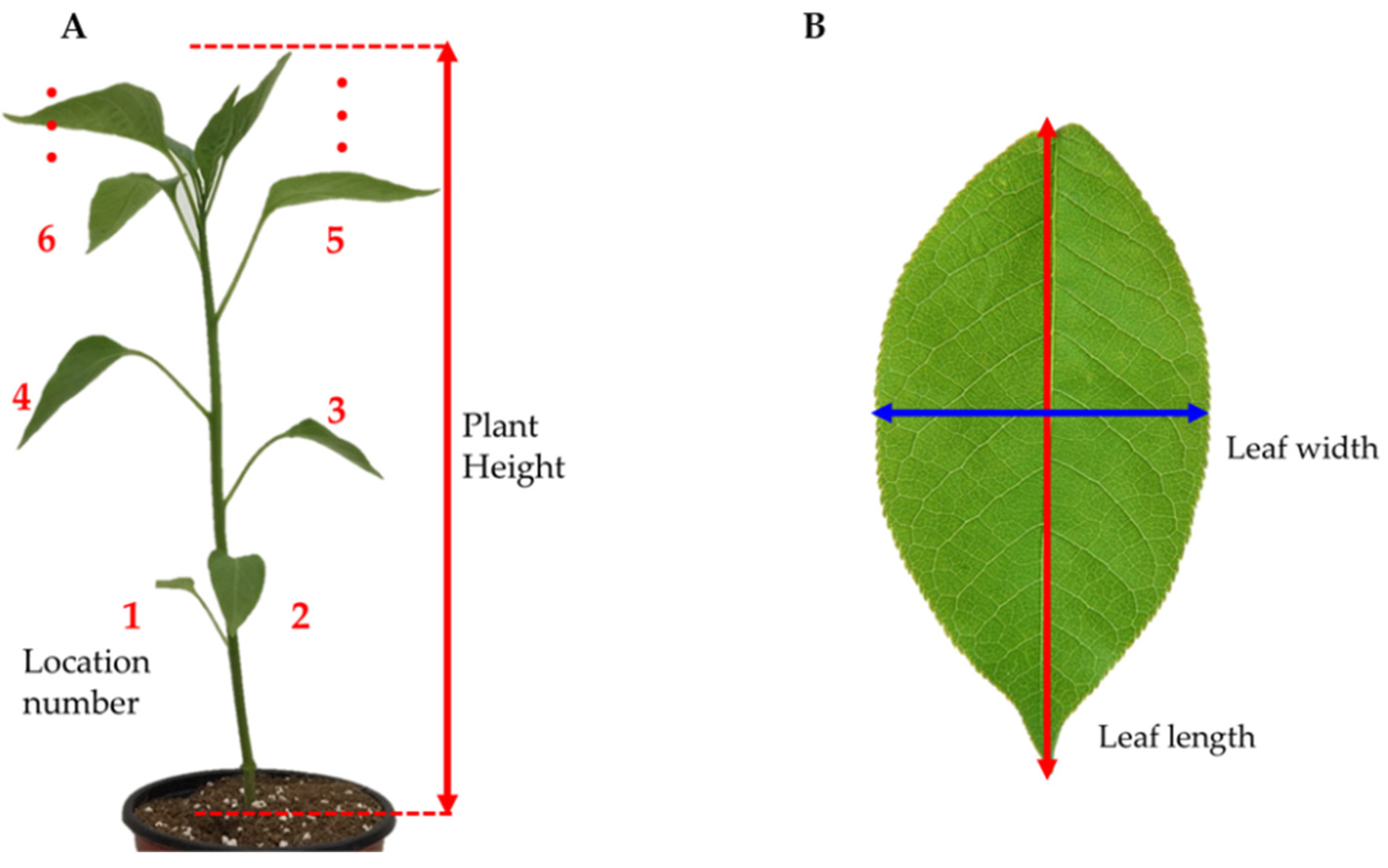
2.3. Measurement Method and Application Software

To examine the model accuracy of the reconstructed 3D image, the height of seedlings and the length and width of all leaves were analyzed. Since the height of crops is related to growth and the size of leaves plays an important role in the photosynthetic process, it was used as an index of plant quality. The crop height was the distance from the pot to the highest part of the seedling and the length and width of the leaves were measured (Figure 2). Each leaf was assigned a number from the bottom and used for analysis. This was called a ‘location number’. When measuring the leaf width, the maximum straight-line distance was measured if the leaf was curved.

The size of each 3D image was analyzed using MeshLab software [34]. The artificially segmented image was measured using MeshLab measurement tool and corrected values were compared with actual measured values. Kinect software development kit, C++, OpenCV library, GMLC++ camera calibration toolbox, and 3D restoration commercial software were used for 3D reconstruction. In addition, Python and MATLAB were used for the segmentation and measurement parts related to automatic analysis of 3D images.

2.4. Algorithm for High-Resolution 3D Reconstruction

Agisoft Photoscan (Agisoft LLC, St.Petersburg, Russia) [35] and visualSfM [36] are representative 3D reconstruction software packages. However, when the target crop was rotated in this experiment, modeling was often performed improperly. Several algorithms were investigated to overcome this problem and obtain high-resolution 3D model data.

Figure 3 shows the flowchart for image acquisition, 3D reconstruction, and analysis. First, depth images and high-resolution RGB images are acquired using the Kinect and an additional smartphone camera mentioned above. Since the acquired depth image has a low resolution, upsampling was performed to overcome this. The resultant upsampled images were matched by camera calibration and image registration with high-resolution images. Matched depth images and color images were used to acquire 3D point cloud data by 3D reconstruction. The 3D crop image data was segmented for each height and leaf manually and the model’s accuracy was analyzed using the actual measured data.

The Kinect’s depth image is very low resolution. This low-resolution image can cause problems such as data loss and inaccurate model generation in subsequent analysis. Image upsampling was performed to overcome this problem. The obtained Kinect depth image was subjected to upsampling using Anisotropic Total Generalized Variation [37]. This algorithm formulated a convex optimization problem using higher order regularization for depth image upsampling. In the optimization process, an anisotropic diffusion tensor calculated from a high-resolution intensity image was used. During the upsampling process, it showed better results than other algorithms with respect to data loss and inappropriate expansion. Excessive image enlargement through upsampling shows the disadvantage of producing inaccurate information rather than the advantage of resolution. Therefore, only twice magnification was used for the width and height.

The RGB, IR sensor of the Kinect and the high-resolution RGB camera cannot be used to photograph from exactly the same position, so the image information does not match. Even if the picture was taken from the same location, the part that is distorted due to the characteristics of the sensor should be considered. Solving this problem requires camera calibration and image registration to be performed. Camera calibration is a method of obtaining camera parameters, and the image registration process helps express different coordinate systems in one coordinate system [38,39]. Camera parameters consist of intrinsic parameters indicating the camera’s internal structure and extrinsic parameters indicating camera direction and position. The intrinsic parameters include the focal length of the lens, the pixel size of the sensor, and the radial distortion factor. A size-aware checkerboard and GML C++ Camera Calibration toolbox were used to obtain these camera parameters. The checkerboard was repeatedly photographed at various angles to extract matching points, thereby deriving the camera parameter values. Several unique points are automatically extracted from each camera image, and knowing the distance between the points makes it possible to estimate internal and external parameters. In general, when there are many images, the estimation is improved, but usually about 20 images is sufficient for the purposes of calibration.

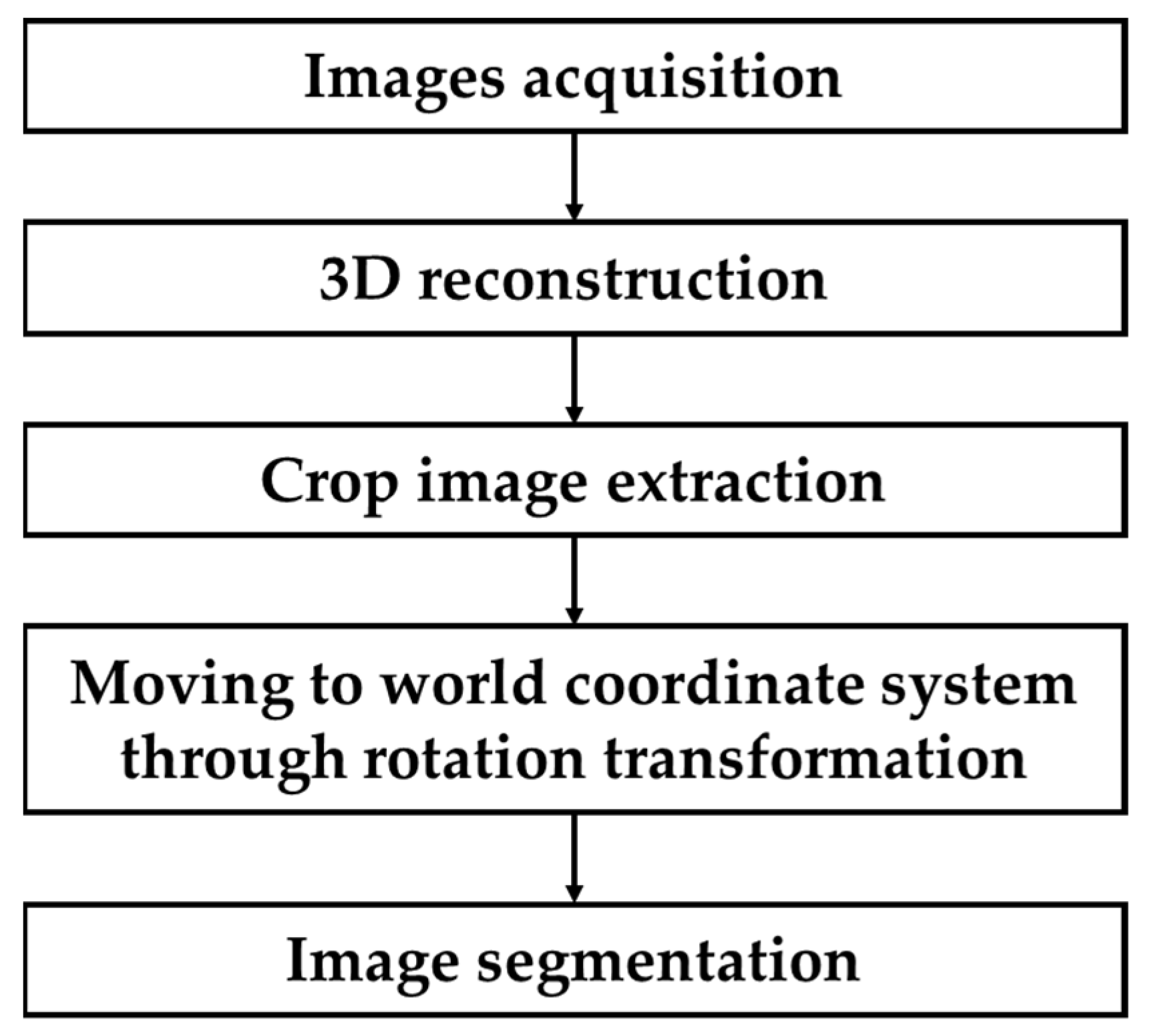
2.5. Machine Learning-Based Crop Extraction and Segmentation Algorithm

2.5.1. 3D Crop Extraction

In order to acquire a 3D image of the crop using the 3D reconstruction algorithm, an attempt was made to develop an automated analysis technique to eliminate errors in the artificial part resulting from human intervention and to increase the reproducibility of the analysis. An algorithm suitable for the reconstructed image was applied for image extraction, which is the process of acquiring the desired part of the image, and image segmentation for dividing it into specific parts. Figure 4 shows the overall flow of the 3D reconstruction process and the further analysis of the 3D image. In Figure 3, all processes after ‘3D image’ were performed manually, but in this section, automatic analysis was performed through the application of various algorithms.

As a result of performing 3D reconstruction of the crop using the above algorithm, a point cloud with 3D coordinates could be obtained. Each point contains coordinate values and color information in 3D space. The reconstructed 3D image contains a small amount of noise information generated during the reconstruction process. It contains background information that is not the target crop, or it might be reconstructed in the wrong location. These parts correspond to various sources of noise that interfere with the analysis and should be removed. In addition, although it cannot be seen as noise, it is necessary to separate out parts that are not related to the morphology of the crop, such as potted plants and soil. In addition, when several 3D-reconstructed crop images are drawn in one coordinate system, they are expressed in various positions and sizes. That is, since the coordinate system and the image scale of the image appear differently depending on the reconstruction process, a correction needs to be performed.

Image extraction to remove parts other than crops, which is the part to be analyzed, started by identifying the characteristics of the data. The 3D point cloud data contains only coordinate and color information, as previously discussed. With this data, it is not possible to distinguish which points correspond to the crop. That is, since the label, which is the explicit correct answer for the 3D image, is not known, the unsupervised learning technique was mainly performed. After applying several machine learning methods, k-means clustering was found to be simple but suitable, and additionally, Otsu’s threshold and vegetation index were used together.

K-means clustering is an algorithm that divides a given data set into k groups, and this group is called a cluster [40]. Because it groups similar types of data together, it is mainly used to discover hidden structures or features in data. The k centroids are assigned to a random location for data on a 2D plane, and a cluster of data is determined according to various distance measurement methods. The centroids are updated using the data belonging to each cluster and repeated until there is no change. Through this process, data can be divided into any number of groups according to the initially specified k. In the 3D crop point cloud, it was used to perform a classification according to color information.

Otsu’s thresholding technique is widely used to process image thresholds [41]. Binarization is the simplest case for separating objects to get information from images. As for what criteria to separate, Otsu provides criteria for setting thresholds using statistical methods. The vegetation index is an index indicating the vitality and growth status of plants, and is used to emphasize vegetation characteristic information. By using this, it can be used as an index that can easily distinguish between crop parts and non-crop parts. The data that can use the vegetation index in the 3D crop image contains information in the visible light band as color values. Accordingly, excess green index (ExG), an index mainly used for analysis through RGB images, was used [42]. As in Equation (1), R, G, and B color channels are used, and the normalized value of each channel divided by the maximum value ($R_m$, $G_m$, $B_m$) is used. At this time, weight is given to green.

$$\begin{gathered} ExG=2g-r-b \\ r=\frac{R^{*}}{R^{*}+G^{*}+B^{*}}, g=\frac{G^{*}}{R^{*}+G^{*}+B^{*}}, b=\frac{B^{*}}{R^{*}+G^{*}+B^{*}} \\ {R}^{*}=\frac{R}{R_m}, G^{*}=\frac{G}{G_m}, B^{*}=\frac{B}{B_m} \end{gathered}$$

(1)

2.5.2. 3D Crop Segmentation and Automatic Analysis

Various algorithms for correction and automatic analysis were applied to the 3D image of the crop part separated through the image extraction algorithm. First, work was carried out to match the coordinate system of several 3D crop images. Coordinate transformation was performed considering the direction of each crop. In the case of scale, it is assumed that there is a certain error in the entire 3D image, and correction was performed using a reference object, the size of which was known. The main algorithms used for this were Principal Component Analysis (PCA) and Euler Angle Transformation.

PCA is an algorithm that finds components that are judged to explain the given data well [43]. The data to be analyzed have many features. The large number of features means that there are many data dimensions, and an increase in the dimensions slows down the learning process, increasing the likelihood of poor performance. Additionally, features include elements that are important to the analysis, as well as elements that are not. Accordingly, it is necessary to reduce the dimensions, and the representative algorithm for this is PCA. PCA performs an algorithm that maximizes data variance. If the PCA algorithm is performed on the given two-dimensional data, PC1, which is judged to be the most important, and PC2, which is the next, can be obtained. In addition to PCA, there are dimensional reduction algorithms such as Linear Discriminant Analysis (LDA) and Independent Component Analysis (ICA), and algorithms are used according to the target direction.

Euler Angle Transformation through Euler Angles and Rotation Matrix can be performed to perform the rotation of objects [44]. The rotation matrix is obtained by using the direction cosine formed by each axis of the reference coordinate system and the rotation coordinate system, and this is multiplied by the coordinate matrix. The conversion equation is as shown in Equation (2), and can be configured by using the rotation angle for each axis

$$\begin{gathered} {\mathrm{A}}^{\prime }=R·A=R_z\left(\alpha \right)R_y\left(\beta \right)R_x\left(\gamma \right) A \\ =\left[\begin{array}{c}c\alpha \\ s\alpha \\ 0\end{array} \begin{array}{c}-s\alpha \\ c\alpha \\ 0\end{array} \begin{array}{c}0\\ 0\\ 1\end{array}\right]\left[\begin{array}{c}c\beta \\ 0\\ -s\beta \end{array}\begin{array}{c}0\\ 1\\ 0\end{array}\begin{array}{c}s\beta \\ 0\\ c\beta \end{array}\right]\left[\begin{array}{c}1\\ 0\\ 0\end{array}\begin{array}{c}0\\ c\gamma \\ s\gamma \end{array}\begin{array}{c}0\\ -s\gamma \\ c\gamma \end{array}\right]·A \\ =\left[\begin{array}{c}c\alpha c\beta \\ s\alpha c\beta \\ -s\beta \end{array}\begin{array}{c}c\alpha s\beta s\gamma -s\alpha c\gamma \\ s\alpha s\beta s\gamma +c\alpha c\gamma \\ c\beta c\gamma \end{array}\begin{array}{c}c\alpha s\beta c\gamma +s\alpha s\gamma \\ s\alpha s\beta c\gamma -c\alpha s\gamma \\ c\beta c\gamma \end{array}\right]·A \end{gathered}$$

(2)

where $R$ is rotation matrix, $s\theta =sin\theta$ and $c\theta =cos\theta$.

Next, to analyze the characteristics of the crop, the 3D crop image should be divided into stems and leaves. The partitioning was attempted using a clustering algorithm. Appropriate parameters were set according to the characteristics of the target stem and leaf, and analysis was performed on a satisfactory individual. In addition to automatic measurement of crop height, automatic calculation of leaf length and width, which are phenotyping features related to leaves, was performed on the image, where stems and leaves were segmented. The measurement criteria were implemented in the same manner as in the 3D image reconstruction accuracy.

As the crop coordinate transformation is performed, the height of crop can be measured as the maximum value of the image z-axis coordinate. Compared to heights where simple measurements are possible, values for leaves require additional processing. The crop coordinate transformation algorithm was additionally performed for the divided leaves. The leaves that performed the PCA algorithm were transformed on the basis of an axis similar to the length vector and an axis similar to the width vector. The length of the leaf was measured by the length of two points with maximum Euclidean distance. The width is measured as the Euclidean distance between the minimum and maximum point coordinates of the axis corresponding to the width. The calculation for each part is as shown in Equation (3).

$$\begin{gathered} h_{crop}=\max \left(\mathit{z}\right) \\ {l}_{leaf}=\max \left\{\left|\stackrel{\rightharpoonup }{p_i-p_j}\right|\right\} \\ {w}_{leaf}=\max \left\{\left|\stackrel{\rightharpoonup }{p_l-p_r}\right|\right\} \end{gathered}$$

(3)

where $\mathit{z}$ is z-axis coordinate value, $p_i$ is i-th point, $p_l$ and $p_r$ are maximum (right) and minimum (left) coordinates on the same axis.

3. Results

3.1. High-Resolution 3D Reconstruction Results

Figure 5 shows the results of performing 3D reconstruction. With respect to the method by which images were obtained in this study, the program using the existing SfM method did not show the 3D reconstruction results; therefore, the results could not be included as comparison images. The Kinect Fusion Explorer on the Kinect SDK provided the overall appearance, but did not seem to display the proper 3D objects. Only the large leaves and potted plants were implemented in 3D form, while the rest were either distorted or appeared in 2D. While it was possible to acquire more accurate 3D objects with low-resolution Kinect color images than with the Kinect Fusion Explorer, it is difficult to perform this analysis. Many leaves were not fully shaped, and were heavily influenced by noise. Finally, using high-resolution RGB images showed that the 3D reconstruction demonstrated good performance overall, except for small parts.

The accuracy of the 3D model was analyzed using the high-resolution 3D reconstruction result image. The number of leaves, the crop height, and the size of leaves were compared with the ground-truth data.

Table 2. Comparison of the number of leaves used in the experiment and the number of leaves that failed to reconstruct.

	Crop
	A	B	C	D
No. of total leaves	30	24	24	26
No. of leaves that failed	2	3	4	4
Successful rate (%)	93.3	87.5	83.3	84.6

shows a comparison of the true values with the reconstructed 3D image. Four seedlings were photographed twice to obtain eight 3D models. In each image, about two leaves have not been reconstructed whatsoever, and few of the very small leaves are depicted.

Table 3. Absolute error, percentage error, and standard deviation between the ground-truth data and the measured values in 3D reconstruction models.

	Crop	Error (cm)	Percentage Error (%)	Standard Deviation	Total Error (cm)	Total Percentage Error (%)	Total Standard Deviation
Leaf length	A	0.139	4.24	0.111	0.183	5.49	0.200
	B	0.233	8.89	0.265
	C	0.189	4.63	0.197
	D	0.187	4.63	0.221
Leaf width	A	0.101	6.30	0.0677	0.124	8.63	0.127
	B	0.149	15.4	0.173
	C	0.173	8.90	0.162
	D	0.084	4.92	0.0805
Crop height	A	0.068	0.313	-	0.344	1.53	0.259
	B	0.314	0.670
	C	0.693	2.74
	D	0.300	1.21

shows the degree of error between the ground-truth data and the measured values in each plant’s 3D reconstruction models. In total, 104 leaves were used for the analysis of the eight 3D models obtained from the four seedlings. The was analyses were divided into whole data and each sample. The error for each seedling was at a similar level, which was attributed to the seedlings being at similar growth stages. Absolute errors were high with respect to leaf width, leaf length, and plant height, depending on the size. The percentage error was the highest for leaf width, which is presumed to have caused several errors due to the method of measuring the straight-line distance of bent leaves.

Overall, the absolute error was low but the characteristics that appeared according to the position or size of the object were further analyzed. Therefore, to understand the underlying cause of errors, an analysis was performed with respect to the location of leaves. The total percentage error value was used to compare the length and width of leaves together. Then, percentage errors were compared for leaves with the same location number (Figure 6). Each plant has a different number of leaves. The red pepper used in the experiment had at least 12~15 leaves. If the location number were greater than 13, the number of data points would be different, and the same location analysis would be difficult. Therefore, analysis was only performed until the 12th leaf. On the graph, each location number should contain eight data points corresponding to four red peppers and two backgrounds. However, since the leaves that did not have a complete 3D shape were excluded, fewer actual points were displayed. The percentage errors were high at the top and bottom of the plant, particularly at the top.

On the basis of the results of the analysis of location number, it was deemed necessary to analyze leaf size. The length, width, and relative areas of leaves were used as indices for leaf size. Since the relative area is composed of a simple product, it is different from the actual leaf area, and the calculation formula for this is as shown in Equation (4):

Relative area = Leaf length × Leaf width

(4)

Figure 7 and Figure 8 show the percentage error for the relative area, length, and width of leaves; the smaller the relative area, the greater the percentage error in both length and width. Similar results were obtained when the length and width were lower, respectively. This means that the smaller the leaves, the more likely it is that reconstruction will fail or that the modeling results will be less complete.

3.2. Crop Image Extraction and Segmentation Results

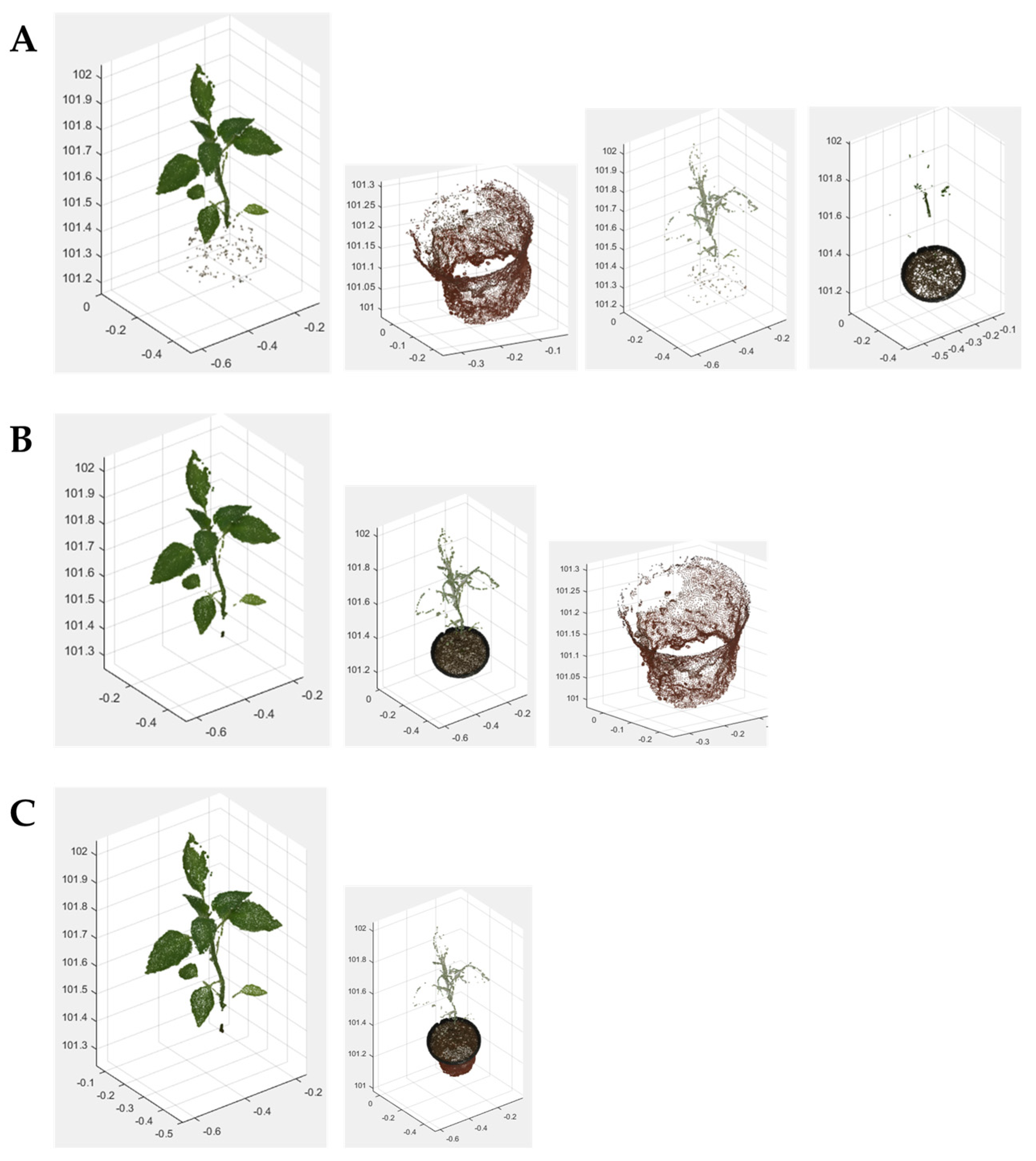
3.2.1. 3D Crop Extraction and Coordinate Transformation

Image extraction was performed by combining several algorithms for the given 3D crop image. Several clustering algorithms were used as unsupervised learning techniques for image extraction. Mean-shift clustering, density-based spatial clustering of applications with noise (DBSCAN), and k-means clustering with differences in k values were compared. In the case of mean-shift clustering, the size of the radius had to be determined, but there was a difficulty in automatic analysis, because it needed to be changed in consideration of the size of the crop. In the case of DBSCAN, there was an advantage in that there were no parameters to be determined in advance, but the extraction itself was not performed properly in many cases. Finally, for k-means clustering, it was necessary to determine the number of classes, k, and although random elements were included in the extraction, the performance was superior to other algorithms. Because it was extraction rather than image segmentation, it was found that the number of classes could be easily pre-determined for both the target crop part and the other parts, and as a result, fewer random elements appeared. Therefore, in subsequent analysis, k-means clustering was used, as it exhibited the best performance. When performing image extraction by combining several additional algorithms, this was confirmed, as shown in Figure 9. When only the color information of the 3D point cloud and k-means clustering were used, the extraction was not performed properly (Figure 9A). Various extractions were possible, depending on the number of clusters, but four—classified into crops, pot, sand, and noise—showed the most optimal results. Nevertheless, various sources of noise remained in the crop part, and various data confirmed that other clusters had not been clearly separated. In addition, because the algorithm contained a random element, we confirmed the instability, with the result being different each time the algorithm was executed. To solve this problem, k-means clustering was performed using the vegetation index value rather than the simple color of the 3D point cloud as shown in Figure 9B. Here, it was performed with three clusters corresponding to the crop, pot, and the rest. Compared to the results of performing only clustering, the crop part was clearly segmented, and other parts were also separated depending on purpose. In the case of configuring the four clusters, the data with respect to the pot and the soil are incomplete, but it can be confirmed that the data were distinguished. Figure 9C shows how to not use clustering. Color information was applied to Otsu’s thresholds. The method employed simple color values and vegetation index for color information. Since the part to be extracted was a crop, it was found that the performance was better when the vegetation index was applied. Accordingly, the vegetation index of ExG was applied to Otsu’s thresholds and analyzed. Because it was a process of binarization, it was divided into crop and non-crop parts. Using this method, it is also possible to extract the crop by properly excluding noise and other parts. Both algorithms using the vegetation index succeeded in extracting crops. There was no significant difference in crop extraction performance. However, when using clustering, since parts other than crops can be further divided, it is expected that additional analysis will be possible compared to the algorithm using the threshold value.

A coordinate system matching process was performed through coordinate transformation of a 3D image of a crop extracted using a combination of algorithms. Figure 10B shows the results of applying the PCA algorithm to the extracted 3D crop image. Components (pc₁, pc₂, …, pc_n) acquired through the PCA sequentially acquire vertical elements on the basis of the first component. On the basis of pc1 (red line), it can be seen that the vertical components are displayed as blue and green lines. Since the pepper used in the experiment is a height-growing crop, pc₁ was found to coincide with the stem direction. Accordingly, Euler Angle Transformation was performed by considering pc1 to be the axis of the crop. Coordinate transformation was performed using pc1 acquired through PCA as the z-axis of the common coordinate system (Figure 10C). The converted image has the bottom of the crop stem as the origin. Through this, the height of the crop can be easily measured, and the degree and direction of differentiation of leaves from the stem can be measured. It also makes it easier to implement segmentation and automatic measurement algorithms. As a result, it was possible to obtain a standardized 3D crop image in a desired format at a constant scale within the same coordinate system.

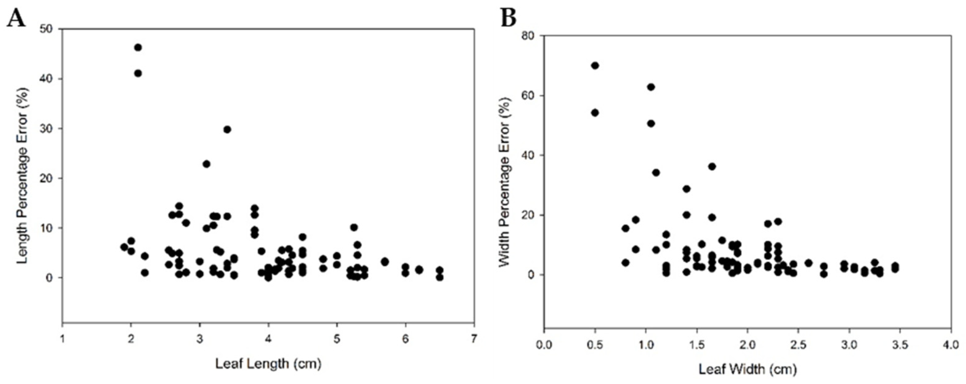
3.2.2. 3D Crop Image Segmentation and Automatic Measurement

The segmentation results for leaves and stems through the clustering algorithm are shown in Figure 11. Regions were divided for the entire 3D crop image, and it was possible to perform independent analysis of each leaf and stem. However, there was no perfect segmentation. While some individuals had properly separated leaves and stems, some parts were not divided, and stems were divided according to specific sizes (Figure 12). If the leaf was too small, or if several individuals were attached very close together, or contained parts that had not been properly restored, proper division could not be achieved.

The data for point cloud leaves that had been successfully segmented were saved separately. The preprocessing carried out in order to apply the automatic measurement algorithm for length and width is shown in Figure 13. When the transformation was performed on the 3D leaf image obtained through the segmentation algorithm, it was possible to obtain results aligned with each of the z- and y-axes for the length and width of the leaf. Since the shape of the leaf is curved rather than flat, differences arise with respect to the actual length and width of the leaf, but there were no problems with the measurement of length and width for the purpose of analysis.

The divided leaves were automatically measured according to the devised length and width measurement method (Figure 14). Distance values were measured for the length (red line) and width (blue line) of the leaves, and compared with actual data using the scale correction value. When looking at the results of the automatic measurement itself before comparing it with the ground truth data, it was found that the desired measurement was made in most cases for the length. However, in the case of the width of the leaves, depending on the degree of restoration, the length of the crooked part, rather than the desired part, was measured and returned as the width, so a high degree of error was expected.

The height, leaf length, and leaf width values obtained via automatic measurement were compared with the actual measured ground true values. Since this is performed using the same sample as that used in the 3D reconstruction accuracy measurement, eight heights for eight 3D crop images and about 50 properly segmented leaves were compared.

The accuracy of the crop height estimations as measured by the error was 4.9 mm, and the total percentage error was 2.2%. This was a little lower than the manually measure results, but there was only a minor difference. As for the results of automatic leaf length measurement in comparison with the ground truth value, the error and total percent error were 2.1 mm and 4.65%, respectively. This error was greater than that for crop height and, moreover, it was greater than the manually measured results. In the case of Figure 15A, the graph of the ground truth value and the manually measured value is shown on the basis of the divided leaves only not the whole leaves, and R² = 0.9584, thus showing better results than using whole leaves. Figure 15B presents a graph of the ground truth value and the automatically measured value, confirming R² = 0.904.

Finally, the leaf width was measured with an error of 4.1 mm and a total percentage error of 18.6%. It was worse than the length of the leaf, and the percentage error, considering its relative size, was very high. Figure 16 presents a graph comparison in the same way as that provided for the leaf length analysis, and it can be seen that the automatically measured leaf width R² was relatively low.

4. Discussion

4.1. 3D Reconstruction

The background being composed of black and white did not appear to affect the results, because the 3D reconstruction process was not significantly affected by lighting [45]. Accordingly, the subsequent results proceeded without considering the background. In addition, images acquired from two directions with respect to the angle of the rotating crop were acquired from all directions with respect to the crop, and this presented no difficulties in recreating the 3D image [18].

The analysis of the error in the reconstructed 3D image was as follows. In the case of small-sized leaves, there were cases in which reconstruction was unsuccessful. Even when reconstructed, the leaves could not be analyzed, because, for example, only part of the leaf was modeled, or it was modeled overlapping with peripheral leaves. A relatively large error appeared at the top and bottom of the crop, which was attributed to the relatively small shooting angles and leaf sizes, in the case of the bottom of the crop. In the upper part of the plant, the leaves were often overlapping or small. With respect to unmodeled leaves, the error is judged to be higher. In addition to the size and position of the leaves, there are other factors to be considered as error. Since the process of collecting data from the turntable to construct the 3D model and that of measuring the actual length were not carried out simultaneously, changes in the curve of the leaf may have occurred due to time change or movement. Since the length of the straight line, rather than the curved length of the leaf, was measured, this was presumed to exert a lot of influence [46].

The results of the 3D reconstruction were analyzed as having a low degree of error, however, there are limitations with respect to the manual measurement of leaf count, length, and width from reconstructed 3D images. Since people are able to count and measure incomplete 3D reconstruction leaves, the error result is judged as being fairly accurate [18]. In addition, the process of manually removing outliers when performing the 3D reconstruction process may have contributed to a reduction in the error. Automation algorithms need to be developed for these processes, and it was found that the accuracy when applying them was lower than that of human measurements. In addition, it is necessary to consider bending when measuring the width of leaves to obtain accurate leaf areas.

4.2. 3D Crop Image Automatic Analysis

In the case of leaves, the degree of inclusion of the node was not constant, making analysis difficult. Since the clustering algorithm used for partitioning contained random elements [47], it seems that a slightly more complete segmentation would be possible only with the addition of other mathematical algorithms.

It was found that the automatic measurement of the segmented part showed better performance than previous studies using a single sensor [48,49]. Because the coordinate transformation exhibited good performance, it was found that the coordinates selected to measure the crop height did not significantly affect the measurement error. The leaves showed a relatively high error compared to the height of the crop. This inferiority in accuracy was attributed to the algorithm not being able to accurately segment the leaves, while there were also differences in the locations to be measured. However, because the small leaves, which were found to cause a large error, were not properly segmented, they were excluded from the analysis, and therefore did not result in a higher degree of error. Basically, the widths of the leaves have smaller values than those of the height of the crop or the length of the leaf; therefore, it is regarded as being a larger error, even with similar values of error. As shown with respect to accuracy of reconstruction, the smaller the size, the greater the influence of the unrestored portion. In addition, as seen in the data analysis performed on the basis of the image, if the point cloud on the side of the leaf is not properly displayed, the value in the diagonal direction, rather than the width in the horizontal direction, will be recognized as the width, inevitably resulting in an increase in error.

5. Conclusions

In this study, the crop image was acquired through 3D reconstruction, and the process of automatically measuring specific information of the crop was performed using the proposed image extraction and segmentation process. The 3D reconstruction system using plant rotation was developed in a laboratory environment. To compensate for the existing reconstruction method, several attempts were made to utilize Kinect depth images and high-resolution color images. As a result, successfully obtaining a high-resolution 3D reconstruction result was possible. However, there is a limitation with respect to the incomplete modeling of small objects and the need to manually process the analysis. To compensate for the manual analysis part, using machine learning algorithms and coordinate transformation, crop images were extracted and segmented, and a reference coordinate system was set. Various algorithms were used to enable the extraction methods to meet the needs of the analysis, and coordinate transformation was performed to ensure consistent analysis. We attempted to segment the extracted image in a simple manner, and the analysis was performed using the designed automatic measurement method, and errors were confirmed. It was found that 3D crop images present large errors for small objects in most cases. The height of the crop and the length of the leaves showed coefficients of determination of 0.9 or higher for the manual measurement, but leaf width was confirmed to be a low value. Accordingly, it is expected that an additional process for elaborate segmentation and automatic measurement is required. Additionally, if a phenotypic analysis experiment is actually conducted using these algorithms, unlike in this paper, it will be necessary to obtain more samples in order to increase the explanatory power. These results confirmed the applicability to various 3D image analyses for high-throughput phenotyping.

References

1. Furbank, R.T.; Tester, M. Phenomics–technologies to relieve the phenotyping bottleneck. Trends Plant Sci. 2011, 16, 635–644. [Google Scholar] [CrossRef]
2. Fahlgren, N.; Gehan, M.A.; Baxter, I. Lights, camera, action: High-throughput plant phenotyping is ready for a close-up. Curr. Opin. Plant Biol. 2015, 24, 93–99. [Google Scholar] [CrossRef] [PubMed] [Green Version]
3. De Fátima da Silva, F.; Luz, P.H.C.; Romualdo, L.M.; Marin, M.A.; Zúñiga, A.M.G.; Herling, V.R.; Bruno, O.M. A diagnostic tool for magnesium nutrition in maize based on image analysis of different leaf sections. Crop Sci. 2014, 54, 738–745. [Google Scholar] [CrossRef]
4. Li, C.; Adhikari, R.; Yao, Y.; Miller, A.G.; Kalbaugh, K.; Li, D.; Nemali, K. Measuring plant growth characteristics using smartphone based image analysis technique in controlled environment agriculture. Comput. Electron. Agric. 2020, 168, 105123. [Google Scholar] [CrossRef]
5. Yahata, S.; Onishi, T.; Yamaguchi, K.; Ozawa, S.; Kitazono, J.; Ohkawa, T.; Yoshida, T.; Murakami, N.; Tsuji, H. A hybrid machine learning approach to automatic plant phenotyping for smart agriculture. In Proceedings of the 2017 International Joint Conference on Neural Networks (IJCNN), Anchorage, AK, USA, 14–19 May 2017; pp. 1787–1793. [Google Scholar]
6. Pound, M.P.; Atkinson, J.A.; Townsend, A.J.; Wilson, M.H.; Griffiths, M.; Jackson, A.S.; Bulat, A.; Tzimiropoulos, G.; Wells, D.M.; Murchie, E.H. Deep machine learning provides state-of-the-art performance in image-based plant phenotyping. Gigascience 2017, 6, gix083. [Google Scholar] [CrossRef]
7. Koh, J.C.; Spangenberg, G.; Kant, S. Automated Machine Learning for High-Throughput Image-Based Plant Phenotyping. Remote Sens. 2021, 13, 858. [Google Scholar] [CrossRef]
8. Sugiura, R.; Tsuda, S.; Tamiya, S.; Itoh, A.; Nishiwaki, K.; Murakami, N.; Shibuya, Y.; Hirafuji, M.; Nuske, S. Field phenotyping system for the assessment of potato late blight resistance using RGB imagery from an unmanned aerial vehicle. Biosyst. Eng. 2016, 148, 1–10. [Google Scholar] [CrossRef]
9. Zheng, J.; Fu, H.; Li, W.; Wu, W.; Yu, L.; Yuan, S.; Tao, W.Y.W.; Pang, T.K.; Kanniah, K.D. Growing status observation for oil palm trees using Unmanned Aerial Vehicle (UAV) images. ISPRS J. Photogramm. Remote Sens. 2021, 173, 95–121. [Google Scholar] [CrossRef]
10. Qiu, R.; Wei, S.; Zhang, M.; Li, H.; Sun, H.; Liu, G.; Li, M. Sensors for measuring plant phenotyping: A review. Int. J. Agric. Biol. Eng. 2018, 11, 1–17. [Google Scholar] [CrossRef] [Green Version]
11. Fourcaud, T.; Zhang, X.; Stokes, A.; Lambers, H.; Körner, C. Plant growth modelling and applications: The increasing importance of plant architecture in growth models. Ann. Bot. 2008, 101, 1053–1063. [Google Scholar] [CrossRef] [Green Version]
12. Snavely, N.; Seitz, S.M.; Szeliski, R. Photo tourism: Exploring photo collections in 3D. ACM Trans. Graph. 2006, 25, 835–849. [Google Scholar] [CrossRef]
13. Li, M.; Zheng, D.; Zhang, R.; Yin, J.; Tian, X. Overview of 3d reconstruction methods based on multi-view. In Proceedings of the 2015 7th International Conference on Intelligent Human-Machine Systems and Cybernetics, Hangzhou, China, 26–27 August 2015; pp. 145–148. [Google Scholar]
14. Remondino, F.; Spera, M.G.; Nocerino, E.; Menna, F.; Nex, F.; Gonizzi-Barsanti, S. Dense image matching: Comparisons and analyses. In Proceedings of the 2013 Digital Heritage International Congress (DigitalHeritage), Marseille, France, 28 October–1 November 2013; pp. 47–54. [Google Scholar]
15. Lou, L.; Liu, Y.; Han, J.; Doonan, J.H. Accurate multi-view stereo 3D reconstruction for cost-effective plant phenotyping. In Proceedings of the International Conference Image Analysis and Recognition, Vilamoura, Portugal, 22–24 October 2014; pp. 349–356. [Google Scholar]
16. Lou, L.; Liu, Y.; Sheng, M.; Han, J.; Doonan, J.H. A cost-effective automatic 3D reconstruction pipeline for plants using multi-view images. In Proceedings of the Conference Towards Autonomous Robotic Systems, Birmingham, UK, 1–3 September 2014; pp. 221–230. [Google Scholar]
17. Jancosek, M.; Pajdla, T. Multi-view reconstruction preserving weakly-supported surfaces. In Proceedings of the CVPR 2011, Colorado Springs, CO, USA, 20–25 June 2011; pp. 3121–3128. [Google Scholar]
18. Ni, Z.; Burks, T.F.; Lee, W.S. 3D reconstruction of small plant from multiple views. In Proceedings of the 2014 Montreal, Quebec, QC, Canada, 13–16 July 2014; p. 1. [Google Scholar]
19. Nguyen, T.T.; Slaughter, D.C.; Townsley, B.; Carriedo, L.; Julin, N.; Sinha, N. Comparison of structure-from-motion and stereo vision techniques for full in-field 3d reconstruction and phenotyping of plants: An investigation in sunflower. In Proceedings of the 2016 ASABE Annual International Meeting, Orlando, FL, USA, 17–20 July 2016; p. 1. [Google Scholar]
20. Yang, Q.; Tan, K.-H.; Culbertson, B.; Apostolopoulos, J. Fusion of active and passive sensors for fast 3d capture. In Proceedings of the 2010 IEEE International Workshop on Multimedia Signal Processing, Saint Malo, France, 4–6 October 2010; pp. 69–74. [Google Scholar]
21. Zhu, J.; Wang, L.; Yang, R.; Davis, J. Fusion of time-of-flight depth and stereo for high accuracy depth maps. In Proceedings of the 2008 IEEE Conference on Computer Vision and Pattern Recognition, Anchorage, AK, USA, 24–26 June 2008; pp. 1–8. [Google Scholar]
22. Lee, E.-K.; Ho, Y.-S. Generation of high-quality depth maps using hybrid camera system for 3-D video. J. Vis. Commun. Image Represent. 2011, 22, 73–84. [Google Scholar] [CrossRef]
23. Paulus, S.; Behmann, J.; Mahlein, A.-K.; Plümer, L.; Kuhlmann, H. Low-cost 3D systems: Suitable tools for plant phenotyping. Sensors 2014, 14, 3001–3018. [Google Scholar] [CrossRef] [PubMed] [Green Version]
24. Wasenmüller, O.; Stricker, D. Comparison of kinect v1 and v2 depth images in terms of accuracy and precision. In Proceedings of the Asian Conference on Computer Vision, Taipei, Taiwan, 20–24 November 2016; pp. 34–45. [Google Scholar]
25. Yang, L.; Zhang, L.; Dong, H.; Alelaiwi, A.; El Saddik, A. Evaluating and improving the depth accuracy of Kinect for Windows v2. IEEE Sens. J. 2015, 15, 4275–4285. [Google Scholar] [CrossRef]
26. Lachat, E.; Macher, H.; Landes, T.; Grussenmeyer, P. Assessment and calibration of a RGB-D camera (Kinect v2 Sensor) towards a potential use for close-range 3D modeling. Remote Sens. 2015, 7, 13070–13097. [Google Scholar] [CrossRef] [Green Version]
27. Gai, J.; Tang, L.; Steward, B. Plant recognition through the fusion of 2D and 3D images for robotic weeding. In Proceedings of the 2015 ASABE Annual International Meeting, New Orleans, LA, USA, 26–29 July 2015; p. 1. [Google Scholar]
28. Gai, J.; Tang, L.; Steward, B. Plant localization and discrimination using 2D + 3D computer vision for robotic intra-row weed control. In Proceedings of the 2016 ASABE Annual International Meeting, Orlando, FL, USA, 17–20 July 2016; p. 1. [Google Scholar]
29. Shah, D.; Tang, L.; Gai, J.; Putta-Venkata, R. Development of a mobile robotic phenotyping system for growth chamber-based studies of genotype x environment interactions. IFAC-PapersOnLine 2016, 49, 248–253. [Google Scholar] [CrossRef]
30. Sun, G.; Wang, X. Three-dimensional point cloud reconstruction and morphology measurement method for greenhouse plants based on the kinect sensor self-calibration. Agronomy 2019, 9, 596. [Google Scholar] [CrossRef] [Green Version]
31. Vázquez-Arellano, M.; Reiser, D.; Paraforos, D.S.; Garrido-Izard, M.; Burce, M.E.C.; Griepentrog, H.W. 3-D reconstruction of maize plants using a time-of-flight camera. Comput. Electron. Agric. 2018, 145, 235–247. [Google Scholar] [CrossRef]
32. Microsoft. Available online: https://developer.microsoft.com/en-us/windows/kinect/hardware (accessed on 14 September 2017).
33. Microsoft. Available online: https://msdn.microsoft.com/en-us/library/dn782025.aspx (accessed on 20 October 2017).
34. Cignoni, P.; Callieri, M.; Corsini, M.; Dellepiane, M.; Ganovelli, F.; Ranzuglia, G. Meshlab: An open-source mesh processing tool. In Proceedings of the Eurographics Italian Chapter Conference, Salerno, Italy, 2–4 July 2008; pp. 129–136. [Google Scholar]
35. PhotoScan. Available online: http://www.agisoft.com/ (accessed on 14 September 2017).
36. Wu, C. VisualSFM: A Visual Structure from Motion System. Available online: http://ccwu.me/vsfm/doc.html (accessed on 14 September 2017).
37. Ferstl, D.; Reinbacher, C.; Ranftl, R.; Rüther, M.; Bischof, H. Image guided depth upsampling using anisotropic total generalized variation. In Proceedings of the IEEE International Conference on Computer Vision, Sydney, Australia, 1–8 December 2013; pp. 993–1000. [Google Scholar]
38. Tsai, R. A versatile camera calibration technique for high-accuracy 3D machine vision metrology using off-the-shelf TV cameras and lenses. IEEE Robot. Autom. 1987, 3, 323–344. [Google Scholar] [CrossRef] [Green Version]
39. Hamzah, R.A.; Salim, S.I.M. Software calibration for stereo camera on stereo vision mobile robot using Tsai’s method. Int. J. Comput. Theory Eng. 2010, 2, 390. [Google Scholar] [CrossRef] [Green Version]
40. Hartigan, J.A.; Wong, M.A. Algorithm AS 136: A k-means clustering algorithm. J. R. Stat. Soc. Ser. C Appl. Stat. 1979, 28, 100–108. [Google Scholar] [CrossRef]
41. Otsu, N. A threshold selection method from gray-level histograms. IEEE Trans. Syst. Man Cybern. Syst. 1979, 9, 62–66. [Google Scholar] [CrossRef] [Green Version]
42. Woebbecke, D.; Meyer, G.; Von Bargen, K.; Mortensen, D. Shape features for identifying young weeds using image analysis. Trans. ASABE 1995, 38, 271–281. [Google Scholar] [CrossRef]
43. Wold, S.; Esbensen, K.; Geladi, P. Principal component analysis. Chemom. Intell. Lab. Syst. 1987, 2, 37–52. [Google Scholar] [CrossRef]
44. Pio, R. Euler angle transformations. IEEE Trans. Automat. Contr. 1966, 11, 707–715. [Google Scholar] [CrossRef]
45. Yemez, Y.; Schmitt, F. 3D reconstruction of real objects with high resolution shape and texture. Image Vis. Comput. 2004, 22, 1137–1153. [Google Scholar] [CrossRef]
46. Golbach, F.; Kootstra, G.; Damjanovic, S.; Otten, G.; van de Zedde, R. Validation of plant part measurements using a 3D reconstruction method suitable for high-throughput seedling phenotyping. Mach. Vis. Appl. 2016, 27, 663–680. [Google Scholar] [CrossRef] [Green Version]
47. Krioukov, D. Clustering implies geometry in networks. Phys. Rev. Lett. 2016, 116, 208302. [Google Scholar] [CrossRef] [PubMed]
48. McCormick, R.F.; Truong, S.K.; Mullet, J.E. 3D sorghum reconstructions from depth images identify QTL regulating shoot architecture. Plant Physiol. 2016, 172, 823–834. [Google Scholar] [CrossRef] [PubMed] [Green Version]
49. Paproki, A.; Sirault, X.; Berry, S.; Furbank, R.; Fripp, J. A novel mesh processing based technique for 3D plant analysis. BMC Plant Biol. 2012, 12, 63. [Google Scholar] [CrossRef] [PubMed] [Green Version]
50. Yang, M.; Cui, J.; Jeong, E.S.; Cho, S.I. Development of High-resolution 3D Phenotyping System Using Depth Camera and RGB Camera. In Proceedings of the 2017 ASABE Annual International Meeting, Spokane, WA, USA, 16–19 July 2017; p. 1. [Google Scholar]
Figure 1. Experimental environment in which various angle images of crops are acquired.
Agriculture 11 01010 g001
Figure 2. Measurement method for the crop and leaves: (A) plant, (B) leaf.
Agriculture 11 01010 g002
Figure 3. Flowchart for image acquisition, 3D reconstruction, and analysis.
Agriculture 11 01010 g003
Figure 4. Flow chart for 3D image acquisition and analysis algorithm.
Agriculture 11 01010 g004
Figure 5. 3D reconstruction results. (A) Kinect fusion explorer, (B) Kinect low-resolution color image, and (C) high-resolution RGB images.
Agriculture 11 01010 g005
Figure 6. Percentage error by leaf position: (A) leaf length and (B) leaf width.
Agriculture 11 01010 g006
Figure 7. Percentage error by leaf relative area; (A) leaf length and (B) leaf width.
Agriculture 11 01010 g007
Figure 8. Percentage error by leaf size: (A) leaf length and (B) leaf width.
Agriculture 11 01010 g008
Figure 9. 3D crop extraction result through combination of several algorithms: (A) k-means clustering (k = 4); (B) ExG + k-means clustering; and (C) ExG + Otsu’s threshold.
Agriculture 11 01010 g009
Figure 10. Coordinate transformation: (A) Original 3D image; (B) PCA performed on a 3D crop image; and (C) standardization of coordinate system through Euler angle transformation.
Agriculture 11 01010 g010
Figure 11. The results of leaf segmentation using the clustering algorithm.
Agriculture 11 01010 g011
Figure 12. 3D point cloud that is divided: (A) leaves, (B) stem, internode, nodes; and (C) elements that failed to segment.
Agriculture 11 01010 g012
Figure 13. Application of transformation algorithm for automatic measurement: (A) basic point cloud of leaves; (B) point cloud of the leaf that has undergone coordinate transformation.
Agriculture 11 01010 g013
Figure 14. Automatic measurement of length and width for segmented leaves.
Agriculture 11 01010 g014
Figure 15. Comparison of automatically measured leaf length with ground truth data: (A) manual measurement and (B) segmentation and automatic measurement.
Agriculture 11 01010 g015
Figure 16. Comparison of automatically measured leaf width with ground truth data: (A) manual measurement and (B) segmentation and automatic measurement.
Agriculture 11 01010 g016