Spatial Distribution of Soil Nutrients in Farmland in a Hilly Region of the Pearl River Delta in China Based on Geostatistics and the Inverse Distance Weighting Method

Abstract

Soil nutrients are essential factors that reflect farmland quality. Nitrogen, phosphorus, and potassium are essential elements for plants, while silicon is considered a “quasi-essential” element. This study investigated the spatial distribution of plant nutrients in soil in a hilly region of the Pearl River Delta in China. A total of 201 soil samples were collected from farmland topsoil (0–20 cm) for the analysis of total nitrogen (TN), available phosphorus (AP), available potassium (AK), and available silicon (ASi). The coefficients of variation ranged from 47.88% to 76.91%. The NSRs of TN, AP, AK, and ASi were 0.15, 0. 07, 0.12, and 0.13, respectively. The NSRs varied from 0.02 to 0.20. All variables exhibited weak spatial dependence (R² < 0.5), except for TN (R² = 0.701). After comparing the prediction accuracy of the different methods, we used the inverse distance weighting method to analyze the spatial distribution of plant nutrients in soil. The uniform spatial distribution of AK, TN overall showed a trend of increasing from northeast to southwest, and the overall spatial distribution of AP and ASi showed that the northeast was higher than the southwest. This study provides support for the delimitation of basic farmland protection areas, the formulation of land use spatial planning, and the formulation of accurate farmland protection policies.

1. Introduction

Soil nutrients are important indicators of cultivated land quality, which is determined by two aspects: soil fertility and spatial location [1]. Soil fertility, which is closely related to the concentrations of soil nutrient elements, is the foundation of soil productivity [2]. Soil nutrient elements can be classified into essential, beneficial, and toxic elements. Essential elements are critical for all plants under all growth conditions, and can be divided into two categories on the basis of their essentiality: (1) macro elements that are required in high amounts, e.g., nitrogen (N), phosphorus (P), and potassium (K), and (2) micro elements that are required in lower amounts, e.g., zinc, manganese, copper, and nickel [3]. Beneficial elements, which usually include sodium, silicon (Si), and cobalt, are vital for some specific plant species growing under certain environmental conditions [4]. A sufficient supply of soil nutrients allows plants to grow and develop normally, and the abundance and chemical form of nutrients directly determines whether the soil is fertile [5]. Therefore, it is essential to measure the concentrations of soil nutrient elements to estimate farmland quality.

Geostatistical methods as a predictive tool have been extensively utilized [6]. There have been many studies of soil nutrient properties in recent years. For example, some studies have assessed soil nutrient conditions in the northeast region of India [2], and predicted their spatial distribution in farmland in Croatia [7]. Similar studies have been conducted in China in Yunnan Province [8], Beijing [9,10], and Shanxi Province [11], as well as in hilly areas of Guangdong [12], Sichuan [13], and Hebei Province [14]. Some researchers have attempted to analyze the spatial variability of soil nutrient properties in farmland in New Zealand [15] and India [16], or in a sandy loam soil in Croatia [17]. In these studies, although different factors were chosen for the evaluations to address different research purposes, the indexes generally included soil organic matter, mineral nutrient elements, and other soil properties, such as pH. Among the mineral nutrient elements, macronutrients have been studied more than micronutrients, especially the essential elements N, P, and K, which are among the most important indicators commonly used to analyze soil fertility.

Silicon is the second most plentiful element in the Earth’s crust, accounting for nearly 29% of the total content of the crust [18]. Generally, Si plays an important role in soil. In aquatic ecosystems, Si along with N and P are the main biogenic elements that maintain net primary productivity (NPP) [19]. Silicon also has a great impact on the growth and development of plants in natural ecosystems due to its unique function of alleviating the deleterious effects of abiotic and biotic stresses in plants [3]. In modern agriculture, Si is recognized as a functional nutrient for rice, sugar cane, etc., and plays an especially important role in the growth and development of Gramineae crops [20]. Within the Poaceae family, rice is the staple food for more than half of the world’s population. Rice plants are Si accumulators and are a high Si demanding crop, usually absorbing Si in greater quantity than essential nutrients such as N, P, K, and Ca [21]. The relationship between increasing rice yield and Si depletion has attracted increasing attention from agricultural scientists [18]. The area studied in the present research has a rich rice yield but is relatively lacking in soil nutrients, partially due to the effects of acid rain, and the absence of Si and various macronutrients (N, P, and K) may limit the rice yield [22].

Soil nutrient properties can vary spatially due to many factors, such as pedogenic processes, climate, parent material, topography, and human influences [15]. When the soil nutrient content exhibits high spatial variability, it is difficult to estimate soil nutrient status among regions based directly on the different geographical features [23]. This study tries to use geostatistics and inverse distance weighting (IDW) methods to explore the problem of soil high spatial. Geostatistics have been widely used to explore spatial uncertainty in recent decades [24]. They can be used to describe the spatial distribution of a variable and to predict its value between sampling points [25]. The IDW method is also commonly used to predict the spatial distribution of soil nutrients. It is a moving weighted-average method that has its optimum effect under conditions in which the sampling points are evenly distributed and not clustered in the sampling area.

In this study, we analyzed the spatial distribution of soil N, P, K, and Si in farmland in Conghua District, Guangzhou, China, using geostatistics and the IDW method. The main objectives of the study were to (i) measure the total nitrogen (TN), available phosphorus (AP), available potassium (AK), and available silicon (ASi); (ii) determine the optimal model fitted and its parameters; and (iii) assess the spatial variability of the selected soil nutrient elements and analyze their spatial distribution.

2. Materials and Methods

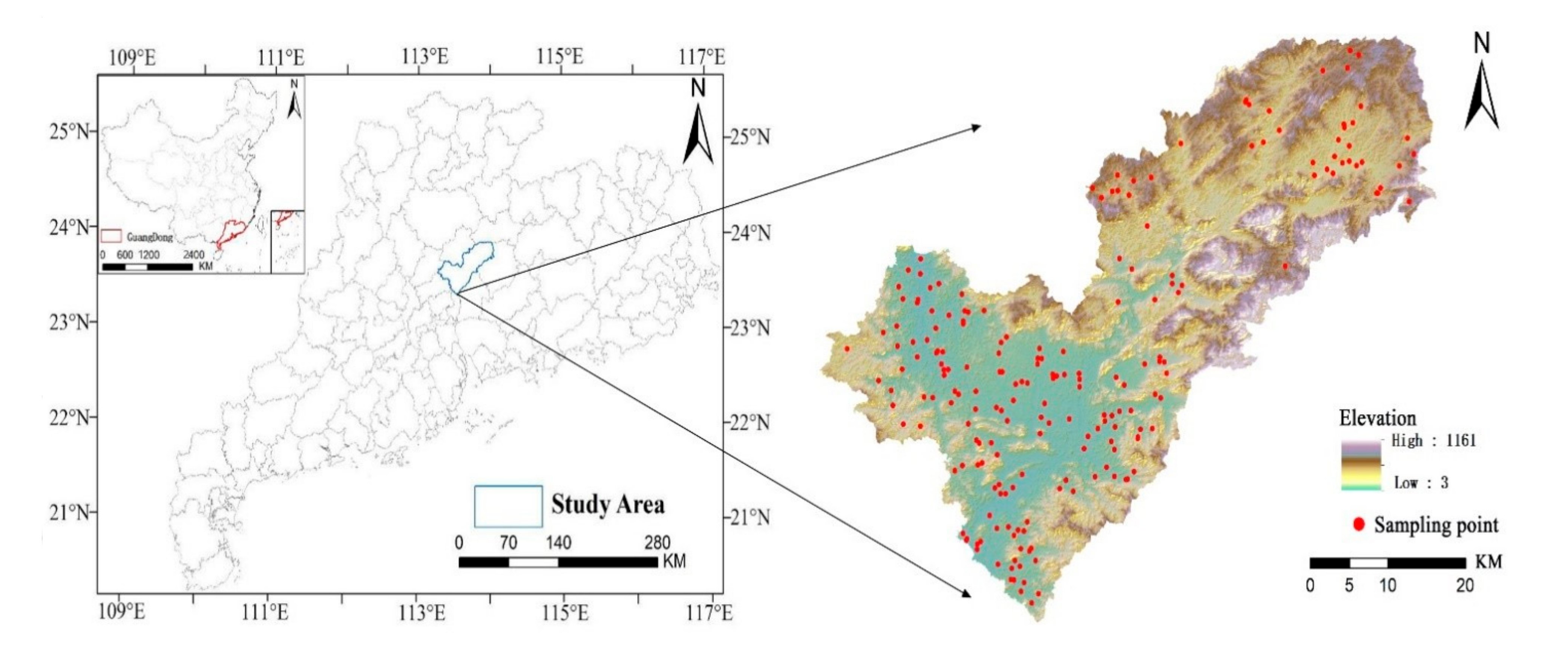
2.1. Study Area, Soil Sampling, and Analysis

The study area was located in the northeast of Guangzhou, in the transition zone from the Pearl River Delta to the mountainous area of northern Guangdong Province, South China (Figure 1). The terrain is tilted from north to south, and the total area of the study area is 1985.3 km². The climate of the study area is Subtropical Monsoon Climate. The mean annual temperature ranges from −1.6 °C in winter to 36.7 °C in summer, and mean annual precipitation is 1930.8 mm. Generally, the soil types can be divided into sandy soil, clayey soil and loam. The United States Department of Agriculture (USDA) Textural Triangle has 12 classes according to the proportion of sand content, viscosity and loam. The study area is located in the plain area of the Pearl River Delta, where the soil has less sediment content, fine particles, slow water seepage rate and general aeration performance. Therefore, the soil types are mainly clay and loam. Due to the cropping system of three crops a year, frequent tillage and high intensity development and utilization activities, the overall situation of soil nutrients in this region is not optimistic.

A total of 201 topsoil samples (0–20 cm) were collected from farmland in the study area for the analysis of their soil nutrient properties. In the sampling: (i) select a large area of farmland; (ii) the sampling point is more than 100 m away from the highway and railway; (iii) avoid the composting edge, irrigation mouth and other places that affect the soil properties [26]. The sample locations were selected according to topography and land use. The sampling density was approximately one sample per 1.07 km² cultivated land. After the weeds and plant roots in the soil had been removed, the topsoil was collected with a small wooden shovel. At each site, five small sub-samples were evenly mixed to create one large composite sample. Finally, the composite sample was placed into a plastic bag, and the condition of the surrounding environment, vegetation, and geographical position was recorded. All specimens were transported to a laboratory for the analysis of soil properties.

The samples were air dried and sieved through a 2-mm sieve for the analysis of soil nutrient elements. The indicators tested included TN, AP, AK, and ASi. TN was determined using the semi-micro Kjeldahl method, AP was extracted with the sodium bicarbonate extraction/molybdenum antimony colorimetric method (Olsen), AK was estimated via ammonium acetate extraction/flame photometry, and ASi was analyzed using a colorimetric method [10].

2.2. Statistical Analysis

Descriptive statistics, including the mean, minimum, maximum, coefficient of variation (CV), and standard deviation, were calculated using SPSS 20.0 [27]. The distribution of the data was tested for normality using the Kolmogorov–Smirnov test, kurtosis, skewness, and percentile–percentile plots. The correlations among the variables were determined based on Pearson’s coefficients, and the CV was used to describe the degree of variation of soil nutrients. A CV of less than 10% indicated weak variability, a CV between 10% and 100% indicated moderate variability, and a CV of more than 100% indicated strong variability [28].

2.3. Geostatistics

Geostatistics were used to analyze the spatial variability of plant nutrients in soil. The approach consists of two stages: the calculation of an experimental variogram from the data and model fitting, and predictions at unsampled locations [24]. A semivariogram is used to measure the spatial variation of regionalized variables [25,29], and is expressed as:

$$\gamma (h)=\frac{1}{2N\left(h\right)}{\displaystyle \sum }_{i=1}^{N\left(h\right)}{[Z\left(xi\right)-Z\left(xi+h\right)]}^2$$

(1)

In Equation (1), γ(h) is the semivariance at a given distance h; Z(xi) is the value of the variable Z at location xi, and N(h) is the number of pairs of sample points separated by the distance h. The variogram plot was fitted with a theorical model, i.e., spherical, exponential, linear, or Gaussian models. The fitted model was selected based on it having both the largest R² and the smallest residual [30], and it could provide information about the spatial structure and the input parameters for the kriging interpolation.

The kriging interpolation method is widely used to research spatial structure and provide estimates of variation at unsampled locations [31]. It includes the concepts of ordinary, simple, universal, probability, indicator, and disjunctive kriging, but the ordinary kriging (OK) method is regarded as the best technique and is known as the linear unbiased estimator.

2.4. The Inverse Distance Weighting Method

The IDW method assumes that a value of an attribute at an unsampled location is a weighted average of known data points, within a local neighborhood surrounding the unsampled location [32]. It is expressed as:

$$\widehat{z}\left(x_0\right)=\frac{{{\displaystyle \sum }}_{i=1}^{n}z\left(xi\right)di{j}^{-r}}{{{\displaystyle \sum }}_{i=1}^{n}di{j}^{-r}}$$

(2)

In Equation (2), $\hat{\mathrm{Z}}$ is estimate value of x₀, which is the estimation point and xi are the data points within a chosen neighborhood. The weights (r) are related to distance by dij, which is the distance between the estimation point and the data points. Higher weights indicate more influence points close to x₀.

2.5. Accuracy Assessment

Cross-verify the accuracy of kriging interpolation using the hold-out method [33] and to help determine the best parameters for the IDW test [31]. The indexes included root-mean-square error (RMSE) and mean-absolute error (MAE), which are be calculated as follows [11]:

$$MAE=\frac{{\displaystyle \sum _{i=1}^N}\left|y\left(xi\right)-y*\left(xi\right)\right|}{N}$$

(3)

$$RMSE=\sqrt{\frac{{\displaystyle \sum _{i=1}^N}{\{y\left(xi\right)-y*\left(xi\right)\}}^2}{N}}$$

(4)

where y(xi) is the measured value, y * (xi) is the predicted value, and N is the number of samples. The best prediction model was obtained when the RMSE and MAE had the smallest value.

3. Results

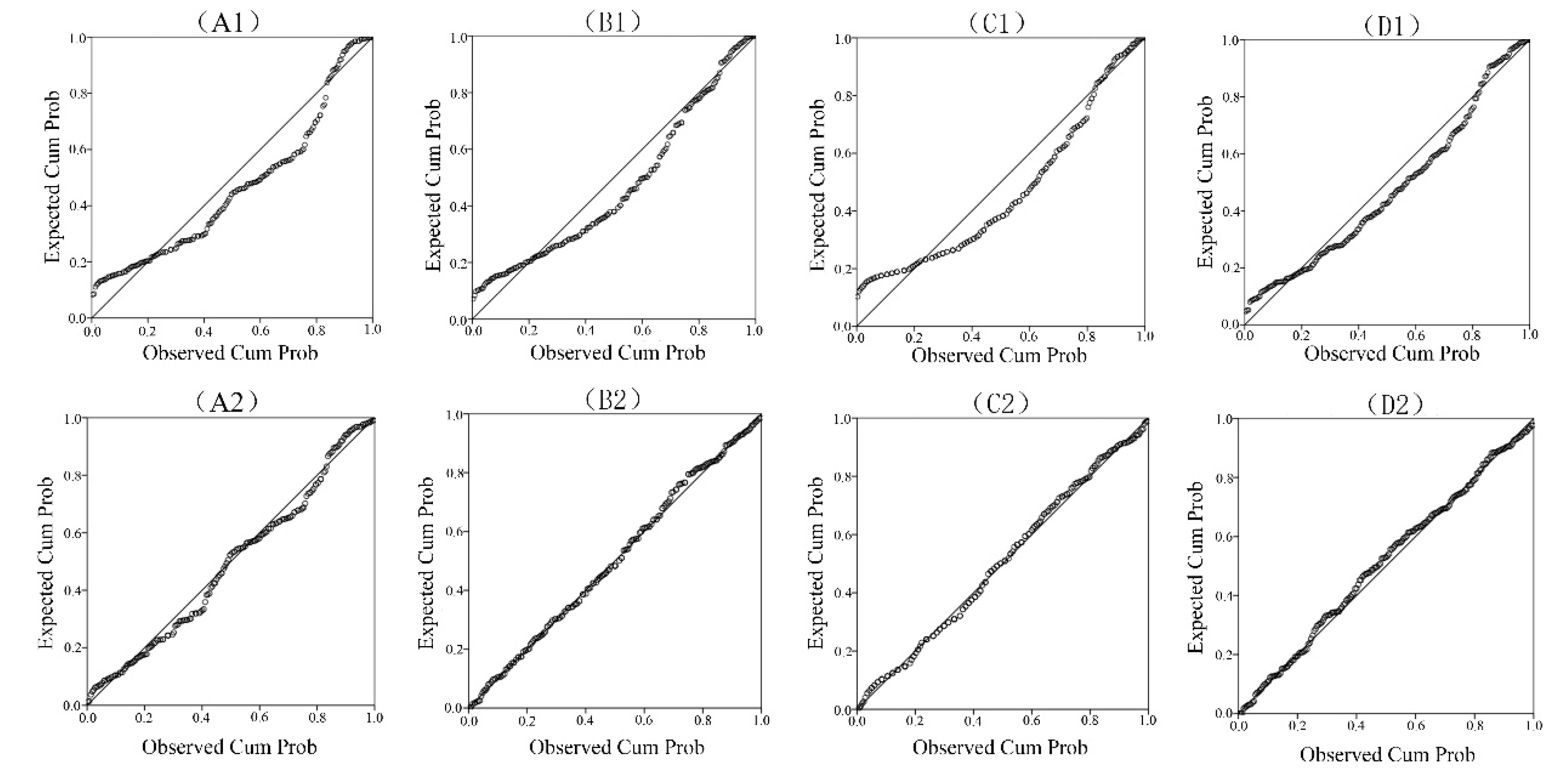
3.1. Descriptive Statistics

As shown in

Table 1. Descriptive statistics of N, P, K and Si in soils.

Variable	Median	Max	Mini	Mean	Std. Dev	Skewnss	Kurtosis	CV %
TN (mg kg−1)	782.00	2140.00	284.00	842.48	403.38	1.28	1.13	47.88
AP (mg kg−1)	35.30	140.80	4.60	43.41	26.48	1.20355	1.36355	60.99
AK (mg kg−1)	60.00	350.00	2.00	77.80	59.84	1.64	3.55	76.91
ASi (mg kg−1)	57.61	170.58	7.55	63.85	33.61	0.90	0.45	52.64

TN, total nitrogen; AP, available phosphorus; AK, available potassium; ASi, available silicon; Max, maximum; Mini, minimum; Std. Dev, standard deviation.

, the average values of TN, AP, AK, and ASi were 842.48 ± 403.38, 43.41 ± 26.48, 77.80 ± 59.84, and 63.85 ± 33.61 mg kg⁻¹, respectively. The CV of TN, AP, AK, and ASi ranged from 47.88% to 76.91%, which indicated a moderate variability for all variables in the study area. The CV values followed the order AK > AP > ASi > TN. TN, AP, and AK displayed moderate variability similar to that found in Hebei [14], Yunnan Province [8], and India [17]. The gradually decreasing trend in the CV among TN, AP, and AK in the study area was similar to that reported in farmland of India [17].

The skewness values of TN, AP, AK, and ASi were 1.28, 1.20, 1.64, and 0.90, respectively. The percentile–percentile plots showed that ASi(D1) was normally distributed, whereas TN(A1), AP(B1), and AK(C1) were non-normally distributed. The Kolmogorov–Smirnov tests demonstrated that all variables followed a normal distribution after logarithmic transformation (Figure 2). There were no significant correlations among TN, AP, AK, and ASi based on the Pearson coefficients.

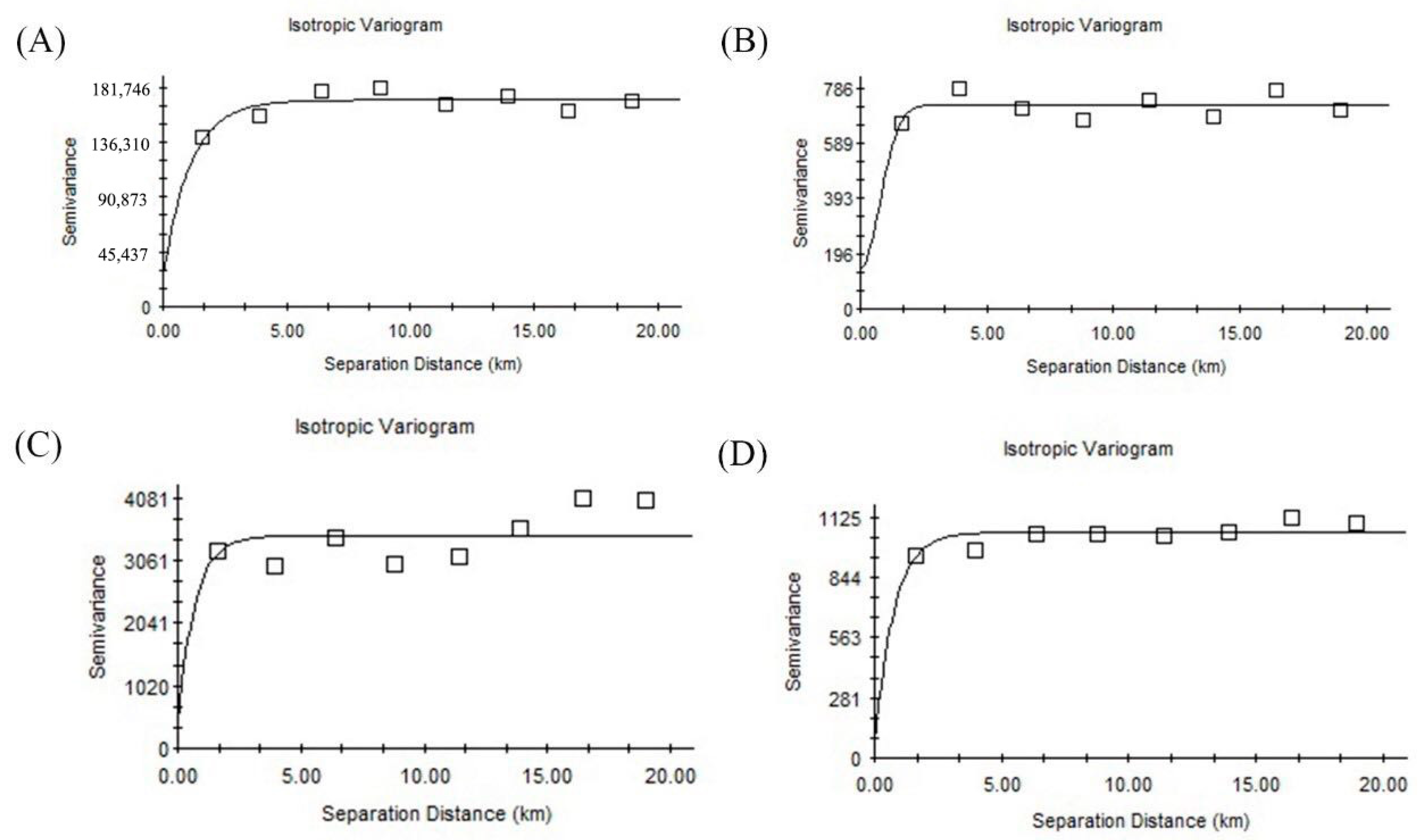
3.2. Ordinary Kriging Results

As shown in

Table 2. Geostatistical analysis of N, P, K and Si in soils.

Variable	Optimal Model	Range (m)	Nugget (C0)	Partial Sill (C)	Sill (C0 + C)	NSR(%)	R2	Residual	Spatial Dependence
TN	Sph	2620	12,200	158,100	170,300	0.08	0.641	4.56E + 08
	Exp *	3300	24,900	146,300	171,200	0.15	0.701	3.81E + 08	weak
	Gau	2269	30,200	140,100	170,300	0.20	0.642	4.55E + 08
AP	Sph *	2190	59	666	725	0.07	0.220	12,154	weak
	Exp	2040	101	623	725	0.13	0.205	12,408
	Gau	1871	144	581	724	0.19	0.221	12,154
AK	Sph	5877	644	2978	3622	0.06	0.095	2,683,579
	Exp *	5530	403	3061	3464	0.12	0.115	2,091,059	weak
	Gau	2934	407	3050	3457	0.15	0.089	2,260,214
ASi	Sph	2270	113	939	1052	0.02	0.410	14,746
	Exp *	2400	140	915	1055	0.13	0.446	13,809	weak
	Gau	1890	103	965	1052	0.10	0.405	14,745

TN, total nitrogen; AP, available phosphorus; AK, available potassium; ASi, available silicon. Sph, spherical model; Exp, exponential model; Gau, Gaussian model; R², R-squared; NSR, nugget to Sill ratio [13,37]. * represents the best fitted model.

, the optimal models were selected based on having the smallest residual and largest R² values. For TN, AK, and ASi, the R² values are 0.701, 0.115 and 0.446, they are both larger than other models, so an exponential model was considered the optimal model, whereas a spherical model was selected as the optimal model for AP (Figure 3).

The ranges of the variograms for AK, ASi, TN, and AP were 5530, 2400, 3300, and 2190 m respectively, which were lower than those reported previously on a similar regional scale [10,11]. Based on the notion that the sampling interval should be less than half the range of the variogram [34] and the principle that sample numbers are usually a compromise between the accuracy required and the resources available for investigation, these results indicated that the sampling design was adequate for determining the spatial variability of soil nutrients in the study area [30].

The nugget (C₀) and sill (C₀ + C) values were used to reflect spatial heterogeneity. C₀ ranged from 59 to 24,900 mg kg⁻¹, whereas C₀ + C varied from 724 to 171,200 mg kg⁻¹. All semivariograms were generally well structured with a small nugget effect, except for TN, indicating that the sampling density was suitable for revealing spatial structures [35]. High C₀ values tend to hide the spatial variation of soil structure [36], but the high nugget effect for TN revealed an irregular distribution of spatial variability.

The nugget-to-sill ratio (NSR) describes the degree of spatial correlation [37]. An NSR less than or equal to 0.25 indicates a weak spatial correlation; an NSR between 0.25 and 0.75 indicates a moderate spatial correlation; and an NSR greater than 0.75 indicates a strong spatial correlation. However, a variable was still considered to have a weak spatial correlation when NSR ≤ 0.25. As shown in Table 2, the NSRs of TN, AP, AK, and ASi were 0.15, 0. 07, 0.12, and 0.13, respectively. All variables had an R² < 0.5, except for TN (R² = 0.701), therefore, they were considered to have weak spatial dependence. These results were similar to previous findings. For example, the spatial correlations of TN and AP in this study area were similar to those reported in a wastewater irrigation area of Beijing and a hilly area of Santai County [10,13].

Spatial variation is generally divided into intrinsic variation and extrinsic variation. Internal changes are caused by structural factors, while external changes are caused by random factors [6,10,33]. The structural factors of internal change include soil texture, soil particle, soil bulk density, etc. The spatial heterogeneity of soil organic matter, total nitrogen, total phosphorus and total potassium was studied by geostatistics method, and it was found that soil structural factors had great influence on soil organic matter, total nitrogen and total potassium, and were simultaneously affected by structural and random factors [13,38]. In general, variables with strong variability are mainly affected by structural factors, while variables with weak variability are affected by random factors. The driving factors of randomness are mainly human factors, such as agricultural irrigation, fertilizer use, tillage measures, etc. In studying the influence of land use change on spatial heterogeneity of soil nutrients in forests in southern Appalachia, Fraterrigo et al. found that land use had a persistent influence on spatial heterogeneity of soil nutrients [33]. All variables in this study belong to moderate variation. Spatial variation of soil nutrients is influenced by both structural and random factors, and has different characteristics in different regions.

3.3. Inverse Distance Weighting Results

In the inverse distance weighting method, root mean squared error (RMSE) indicates that the smaller the values, the better the model prediction. The minimum RMSE was observed when p = 1, and the maximum when p = 3 (

Table 3. Inverse distance weight analysis of N, P, K and Si in soils.

Indicator	Model	TN	AP	AK	ASi
RMSE	p = 1	404.51	26.85	58.63	31.50
	p = 2	419.06	27.60	61.38	32.26
	p = 3	440.41	28.63	64.30	33.51

TN, total nitrogen; AP, available phosphorus; AK, available potassium; ASi, available silicon. RMSE, root mean squared error. p = 1, 2, 3, represent different expectations.

). When p = 1, the RMSEs of TN, AP, AK, and ASi were 404.51, 26.85, 58.63 and 31.50, and when p = 3 the RMSEs of TN, AP, AK, and ASi ranged from 28.63 to 440.41, respectively. The RMSE values followed the order TN > AK > ASi > AP.

3.4. Evaluation of Prediction Methods

Cross-validation was used to validate the accuracy of spatial interpolation. The best prediction models for the variables were selected based having the lowest RMSE and MAE values (

Table 4. Modeling precision of OK and IDW methods for N, P, K and Si in soils.

Variable	Method	Model	ME	MAE	RMSE
TN	OK	Sph	−0.01	163.90	15.49
		Exp *	0.57	154.47	14.64
		Gau	−0.20	175.67	16.57
	IDW	p = 1 *	−0.68	9.21	4.25
		p = 2	−1.49	16.76	4.37
		p = 3	−3.87	91.72	9.33
AP	OK	Sph *	0.23	10.96	14.30
		Expl	0.25	12.25	15.99
		Gau	0.26	12.17	15.90
	IDW	p = 1 *	0.00	0.45	0.15
		p = 2	0.01	1.08	0.18
		p = 3	0.04	6.70	0.65
AK	OK	Sph	−1.35	25.31	32.70
		Exp *	−1.19	21.71	28.18
		Gau	——	——	——
	IDW	p = 1 *	0.01	1.03	0.34
		p = 2	0.12	2. 42	0.40
		p = 3	0.31	13.96	1.41
ASi	OK	Sph	−0.86	18.30	23.52
		Exp *	−0.57	13.87	17.98
		Gau	−0.90	18.96	24.35
	IDW	p = 1 *	0.15	0.44	0.18
		p = 2	0.15	1.22	0.23
		p = 3	−0.02	7.68	0.77

TN, total nitrogen; AP, available phosphorus; AK, available potassium; ASi, available silicon. Sph, spherical model; Exp, exponential model; Gau, Gaussian model; * represent the best predicted model; ME, mean error; MAE, mean absolute error; RMSE, root-mean-square error; OK, ordinary kriging; IDW, inverse distance weighting.

). Thus, the exponential model was selected for TN, AK, and ASi, whereas the spherical model was selected for AP. The mean errors of TN, AP, AK, and ASi were 0.57, 0.23, −1.19, and −0.57, respectively; the negative values indicated that the predicted values of AK and ASi were less than the experimental values. Based on their having the lowest RMSE and MAE, the best prediction models were selected when p = 1 using IDW. The mean errors of TN, AP, AK, and ASi were −0.68, 0, 0.01, and 0.15, respectively; the negative value indicated that the predicted value of TN was less than the experimental value.

The estimation of soil properties is one of the most challenging problems in geoscience [39]. Studies have found that using the RMSE as an indicator can have disadvantages, especially in the process of verifying the models generated by different interpolation methods [40]. In this study, we selected the RMSE and MAE as indicators to assess the interpolation accuracy when the same method was applied to the data, e.g., OK or IDW, and used the indicators of optimal accuracy (IOA) and imprecision (IP) to evaluate the predicted accuracy when different interpolation methods were applied to the same data [41]; the formulas are as follows:

$$IOA=\left|\frac{{\displaystyle \sum _{i=1}^n}{(Zi-\widehat{Z}i)}^2}{{\displaystyle \sum _{i=1}^n}\left(\left|Zi-\overline{X}\right|+\left|Zi-\overline{Y}\right|\right)}\right|$$

(5)

$$IP\left(x0\right)=RMS{E}^2\left(x_0\right)-M{E}^2\left(x_0\right)$$

(6)

As shown in

Table 5. Comparison of interpolated accuracy of different interpolation methods.

Methods	Indicator	TN	AP	AK	ASi
IDW	IOA	6.07	0.11	0.26	0.13
	IP	17.56	0.02	0.12	0.01
OK	IOA	87.74	6.27	10.79	7.67
	IP	214.13	0.96	2.54	1.29

TN, total nitrogen; AP, available phosphorus; AK, available potassium; ASi, available silicon; IP, imprecision; IOA, index of optimal accuracy; IDW, inverse distance weight; OK, ordinary kriging.

, the IOAs of TN, AP, AK, and ASi obtained from IDW were 6.07, 0.11, 0.26, and 0.13, respectively. The IOAs of TN, AP, AK, and ASi obtained from IDW were less than those obtained from OK, indicating that the predicted accuracies of IDW were higher than those of OK. The IPs of TN, AP, AK, and ASi obtained from OK were 214.13, 0.96, 2.54, and 1.29, respectively. The IP values of TN AP, AK, and ASi obtained from OK were larger than those obtained from IDW, indicating that the predicted accuracies of IDW were higher than those of OK. Therefore, we concluded that the prediction accuracy of TN, AP, AK, and ASi obtained from IDW was higher than that obtained from OK. Therefore, we used IDW to analyze the spatial distribution of soil nutrient elements.

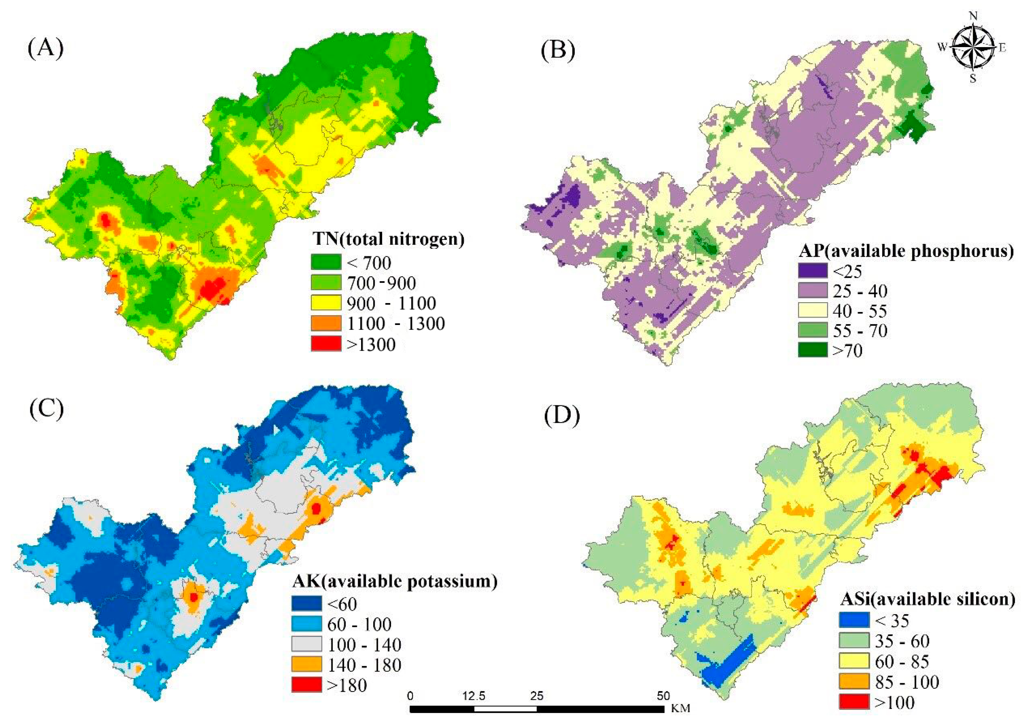
3.5. Spatial Distribution of Soil Nutrient Elements

The spatial distributions of TN, AP, AK and ASi were plotted using the ArcGIS 10.2 software, and the results are shown in Figure 4. TN displayed an overall increasing trend from the northeast to southwest in the range of 493.28 to 1529.56 mg kg⁻¹. The TN content was generally low (<700 mg kg⁻¹) to moderate (700–1100 mg kg⁻¹) in most areas, and it was only high (>1100 mg kg⁻¹) in some scattered locations that represented 6.65% of the total area. It may be due to the influence of topographic factors. In northeast China, most areas are mountainous with high altitude and steep slope, while in southwest China, there are plain areas with low altitude. The AP content was low (25–40 mg kg⁻¹) to moderate (40–55 mg kg⁻¹) in most regions, and was generally higher in the northeast than the southwest. This is because areas with high total nitrogen content are located around urban areas, and the use of human factors on land is significantly higher than other areas. The AK content exhibited an even distribution across the study area, with no significant regional features. The AK content varied from 21.30 to 244.26 mg kg⁻¹, and was very low (<108 mg kg⁻¹) in 99.66% of the total area. ASi exhibited a similar spatial distribution as AP. The ASi content was moderate (60–85 mg kg⁻¹) to low (35–60 mg kg⁻¹) in most regions, and most soils in the study area showed ASi deficiency. The overall low content of AK and ASi may be due to the fact that frequent human land use activities have destroyed the soil cultivation layer, resulting in the lack of soil nutrients, especially in the urbanized areas of the southwest, where the more intense land development and utilization activities, the more obvious.

4. Discussion

The purpose of this paper was mainly to discuss the spatial distribution features of soil nutrients at the county scale, so that to understand the spatial variation of soil nutrients and master the influencing factors in the evolution process, to provide a scientific proof for formulating reasonable plan of land use management and a technical support for precision agriculture.

In this paper, kriging and inverse distance weight interpolation methods were used to analyze the spatial distribution features of plant nutrients in soil, and the optimal model and the optimal parameters of different methods were obtained in the study area. Based on these, a series of quantitative indicators were used to discuss the forecast results of different models. That was an innovative attempt in the thinking of plant nutrients in soil analysis because of many studies focus only on one method in the past [6,9,10,13]. The results showed that TN is moderately enriched and AP is deficient in the study area, which was consistent with the geochemical survey results. Secondly, in the selection of research objects, there are few studies on discussing ASi together with AN, AP and AK. In this study [42], the spatial distribution features of these soil nutrients were discussed according to the characteristics of regional natural geography and crop planting in the studied area, which was helpful to fully understand the soil nutrients and make a measure for precision agriculture [3,6].

Plant nutrients content in soil is caused by both natural and human factors. Most researches showed that parent material has the most significant effect on soil formation and soil nutrient content, and soil nutrient content is also closely related to climate, rainfall, vegetation, land use types and agricultural production measures [43]. It is well known that soil parent materials are the material carriers and there are differences in soil nutrients for the difference of parent materials [2,19,43]. It commonly existed a significant correlation between parent material and soil nutrients, that is, the higher the mineral element content of soil parent material, the higher the content of plant nutrients in soil in the corresponding area. Soil types are mainly caused by different parent materials. The influences of human activities on soil nutrients are mainly showed in agricultural production, the spatial distribution of soil nutrients will be affected by different fertilization methods and land use types.

The study area is located in the hilly area of Southeast China, granite is the main soil parent material, and the soil types are mainly clay and loam [44]. Many paddy fields are planted with rice, and dry lands are planted with dry crops such as peanuts. Located in the edge of Pearl River Delta urban agglomeration, land value is very high and land use is frequent, so that the spatial variability of plant nutrients in soil were simultaneously affected by structural and random factors [13,37]. In this paper, the soil sampling was selected according to topography, land use types and vegetation conditions, and the sampling points covered the main soil types. The analyzed conclusions were consistent with the geochemical survey results.

5. Conclusions

Results showed that the overall content of the spatial distribution of TN, AP, AK, ASi in the study area is relatively low. In addition to the uniform spatial distribution of AK, TN overall showed a trend of increasing from northeast to southwest, and the overall spatial distribution of AP and ASi showed that the northeast was higher than the southwest. Therefore, measures should be taken to increase the content of TN, AP, AK, ASi in the soil of the study area. According to the requirements of different crops for the content of TN, AP, AK, and ASi, it can be planted in districts according to local conditions. Thus, understanding of the spatial distribution characteristics of soil nutrient content in the study area can not only adapt to local conditions and promote the development of agricultural production, but also provide guidance for the delineation of basic farmland protection areas, land use spatial planning and the formulation of accurate farmland protection policies.

References

1. Zhao, D.H.; Guo, C. The thinking of problems of cultivated land appraisal. China Land 1997, 11, 18–19. [Google Scholar]
2. Padua, S.; Chattopadhyay, T.; Bandyopadhyay, S.; Ramchandran, S.; Jena, R.K.; Ray, P.; Roy, P.D.; Baruah, U.; Sah, K.D.; Singh, S.K.; et al. A simplified soil nutrient information system: Study from the north east region of india. Curr. Sci. 2018, 114, 1241–1249. [Google Scholar] [CrossRef]
3. Imtiaz, M.; Rizwan, M.S.; Mushtaq, M.A.; Ashraf, M.; Shahzad, S.M.; Yousaf, B.; Saeed, D.A.; Rizwan, M.; Nawaz, M.A.; Mehmood, S.; et al. Silicon occurrence, uptake, transport and mechanisms of heavy metals, minerals and salinity enhanced tolerance in plants with future prospects: A review. J. Environ. Manag. 2016, 183, 521–529. [Google Scholar] [CrossRef] [PubMed] [Green Version]
4. Bakhat, H.F.; Bibi, N.; Zia, Z.; Abbas, S.; Hammad, H.M.; Fahad, S.; Ashraf, M.R.; Shah, G.M.; Rabbani, F.; Saeed, S. Silicon mitigates biotic stresses in crop plants: A review. Crop Prot. 2018, 104, 21–34. [Google Scholar] [CrossRef]
5. Huang, C.Y. Soil Science; China Agriculture Press: Beijing, China, 2000. [Google Scholar]
6. Kingsley, J.; Lawani, S.O.; Esther, A.O.; Ndiye, K.M.; Sunday, O.J.; Penížek, V. Predictive Mapping of Soil Properties for Precision Agriculture Using Geographic Information System (GIS) Based Geostatistics Models. Mod. Appl. Sci. 2019, 10, 60–77. [Google Scholar] [CrossRef] [Green Version]
7. Bogunovic, I.; Pereira, P.; Brevik, E.C. Spatial distribution of soil chemical properties in an organic farm in Croatia. Sci. Total Environ. 2017, 584–585, 535–545. [Google Scholar] [CrossRef] [Green Version]
8. Li, C.; Li, W.F.; Observatory, Y.M. Study on the relations between the spatial distribution of plateau cultivated soil nutrients and impact factors. Chin. J. Soil Sci. 2014, 45, 1113–1118. [Google Scholar]
9. Wu, Q.; Zou, G.Y.; Shi, Z.P.; Bi, X.Q.; Du, L.F. Soil nutrient status and spatial distribution characteristics of farmland in Beijing east-south suburb. North. Hortic. 2015, 23, 173–178. [Google Scholar]
10. Bao, Z.; Wu, W.; Liu, H.; Yin, S.; Chen, H. Geostatistical analyses of spatial distribution and origin of soil nutrients in long-term wastewater-irrigated area in Beijing, China. Acta Agric. Scand. Sect. B-Soil Plant Sci. 2014, 64, 235–243. [Google Scholar] [CrossRef]
11. Yang, Y.C.; Yang, L.A.; Wang, J.; Wang, A.L.; Huang, A.; Zhang, B.; Xiang, Y.; Wang, Z.Y. Prediction for spatial distribution of soil nutrients based on multiple linear regression model-a case study in lantian county of Shaanxi Province. Chin. J. Soil Sci. 2017, 48, 1102–1113. [Google Scholar]
12. Egbuche, C.T.; Zhiyoa, S.; Anyanwu, J.C.; Onweremadu, E.U.; Nwaihu, E.C.; Umeojiakor, A.O.; Ibe, A.E. Spatial Patterns of Nutrient Distribution in Dalingshan Forest Soil of Guangdong Province China. Agric. For. Fish. 2015, 4, 1–4. [Google Scholar]
13. Li, Q.-Q.; Zhang, X.; Wang, C.; Li, B.; Gao, X.-S.; Yuan, D.-G.; Luo, Y.-L. Spatial prediction of soil nutrient in a hilly area using artificial neural network model combined with kriging. Arch. Agron. Soil Sci. 2016, 62, 1541–1553. [Google Scholar] [CrossRef]
14. Li, X.S.; Xu, Z.Q.; Zhao, Y.; Li, X. Spatial heterogeneity of surface soil nutrient and soil depth in dry south-slope of North Mountain of Hebei. J. Hebei Agric. Univ. 2018, 41, 24–30. [Google Scholar]
15. Qiu, W.; Curtin, D.; Johnstone, P.; Beare, M.; Hernandez-Ramirez, G. Small-scale spatial ariability of plant nutrients and soil organic matter: An arable cropping case study. Commun. Soil Sci. Plant Anal. 2016, 47, 2189–2199. [Google Scholar] [CrossRef]
16. Vasu, D.; Singh, S.; Sahu, N.; Tiwary, P.; Chandran, P.; Duraisami, V.; Ramamurthy, V.; Lalitha, M.; Kalaiselvi, B. Assessment of spatial variability of soil properties using geospatial techniques for farm level nutrient management. Soil Tillage Res. 2017, 169, 25–34. [Google Scholar] [CrossRef]
17. Bogunovic, I.; Mesic, M.; Zgorelec, Z.; Jurišić, A.; Bilandžija, D. Spatial variation of soil nutrients on sandy-loam soil. Soil Tillage Res. 2014, 144, 174–183. [Google Scholar] [CrossRef]
18. Cuong, T.X.; Ullah, H.; Datta, A.; Hanh, T.C. Effects of Silicon-Based Fertilizer on Growth, Yield and Nutrient Uptake of Rice in Tropical Zone of Vietnam. Rice Sci. 2017, 5, 283–290. [Google Scholar] [CrossRef]
19. Xing, J.; Song, J.; Yuan, H.; Li, X.; Li, N.; Duan, L.; Kang, X.; Wang, Q. Fluxes, seasonal patterns and sources of various nutrient species (nitrogen, phosphorus and silicon) in atmospheric wet deposition and their ecological effects on Jiaozhou Bay, North China. Sci. Total Environ. 2017, 576, 617–627. [Google Scholar] [CrossRef]
20. Pati, S.; Pal, B.; Badole, S.; Hazra, G.C.; Mandal, B. Effect of Silicon Fertilization on Growth, Yield, and Nutrient Uptake of Rice. Commun. Soil Sci. Plant Anal. 2016, 47, 284–290. [Google Scholar] [CrossRef]
21. Marxen, A.; Klotzbucher, T.; Jahn, R.; Kaiser, K.; Nguyen, V.S.; Schmidt, A.K.; Schadler, M.; Vetterlein, D. Interaction between silicon cycling and straw decomposition in a silicon deficient rice production system. Plant Soil 2016, 398, 1–11. [Google Scholar] [CrossRef]
22. Malav, J.K.; Ramani, V.P.; Sajid, M.; Kadam, G.L. Influence of Nitrogen and Silicon Fertilization on Yield and Nitrogen and Silicon uptake by Rice (Oryza Sativa L.) under Lowland Conditions. Res. J. Chem. Environ. 2017, 21, 45–49. [Google Scholar]
23. Loescher, H.; Ayres, E.; Duffy, P.; Luo, H.; Brunke, M. Spatial variration in soil properties among north american ecosystems and guidelines for sampling designs. PLoS ONE 2014, 9, e83216. [Google Scholar] [CrossRef] [PubMed] [Green Version]
24. Burgos, P.; Madejón, E.; Pérez-De-Mora, A.; Cabrera, F. Spatial variability of the chemical characteristics of a trace-element-contaminated soil before and after remediation. Geoderma 2006, 130, 157–175. [Google Scholar] [CrossRef]
25. Mabit, L.; Bernard, C. Assessment of spatial distribution of fallout radionuclides through geostatistics concept. J. Environ. Radioact. 2007, 97, 206–219. [Google Scholar] [CrossRef]
26. Jabro, J.D.; Stevens, W.B.; Evans, R.G.; Iversen, W.M. Spatial Variability and Correlation of Selected Soil Properties in the Ap Horizon of a CRP Grassland. Appl. Eng. Agric. 2010, 26, 419–428. [Google Scholar] [CrossRef] [Green Version]
27. Duffera, M.; White, J.G.; Weisz, R. Spatial variability of southeastern U.S. coastal plain soil physical properties: Implications for site-specific management. Geodema 2007, 137, 327–339. [Google Scholar] [CrossRef]
28. Zheng, H.L.; Chen, J.; Deng, W.J.; Tan, M.Z. Assessment of soil heavy metals pollution in the chemical industrial areas of Nanjing peri-urban zone. Acta Sci. Circumstantiae 2005, 25, 1182–1188. [Google Scholar]
29. Goovaerts, P. Geostatistics in soil science: State-of-the-art and perspectives. Geodema 1999, 89, 1–45. [Google Scholar] [CrossRef]
30. Mabit, L.; Bernard, C. Spatial distribution and content of soil organic matter in an agricultural field in eastern Canada, as estimated from geostatistical tools. Earth Surf. Process Landf. 2010, 35, 278–283. [Google Scholar] [CrossRef]
31. Heuvelink, G.B.M.; Webster, R. Modelling soil variation: Past, present, and future. Geodema 2001, 100, 269–301. [Google Scholar] [CrossRef]
32. Robinson, T.P.; Metternicht, G. Testing the performance of spatial interpolation technique for mapping soil properties. Comput. Electron. Agric. 2005, 50, 97–108. [Google Scholar] [CrossRef]
33. Fraterrigo, J.M.; Turner, M.G.; Pearson, S.M.; Dixon, P. Effects of past land use on spatial heterogeneity of soil nutrients in southern appalachian forests. Ecol. Monogr. 2005, 75, 215–230. [Google Scholar] [CrossRef]
34. Kerry, R.; Oliver, M.A. Average variograms to guide soil sampling. Int. J. Appl. Earth Obs. Geoinf. 2004, 5, 307–325. [Google Scholar] [CrossRef]
35. McGratha, D.; Zhang, C.S.; Carton, O.T. Geostatistical analyses and hazard assessment on soil lead in Silvermines area, Ireland. Environ. Pollut. 2004, 127, 239–248. [Google Scholar] [CrossRef]
36. Wang, J.; Yang, R.X.; Bai, Z.K. Spatial variability and sampling optimization of soil organic carbon and total nitrogen for Minesoils of the Loess plateau using geostatistics. Ecol. Eng. 2015, 82, 159–164. [Google Scholar] [CrossRef]
37. Cambardella, C.A.; Moorman, T.B.; Novak, J.M.; Parkin, T.B.; Karlen, D.L.; Turco, R.F.; Konopka, A.E. Field-scale variability of soil properties in central lowa soils. Soil Sci. Soc. Am. J. 1994, 58, 1501–1511. [Google Scholar] [CrossRef]
38. Zhou, H.H.; Chen, Y.N.; Li, W.H. Soil properties and their spatial pattern in an oasis on the lower reaches of the Tarim River, northwest China. Agric. Water Manag. 2010, 97, 1915–1922. [Google Scholar] [CrossRef]
39. Sohrabian, B.; Tercan, A.E. Introducing minimum spatial cross-correlation kriging as a new estimation method of heavy metal contents in soils. Geoderma 2014, 226–227, 317–331. [Google Scholar] [CrossRef]
40. Shi, W.J.; Yue, T.X.; Shi, X.L.; Song, W. Research progress on spatial interpolation methods and their accuracy of soil continuous properties. Chin. J. Nat. Resour. 2012, 27, 163–175. [Google Scholar]
41. Liu, T.L.; Juang, K.W.; Lee, D.Y. Interpolating Soil Properties Using Kriging Combined with Categorical Information of Soil Maps. Soil Sci. Soc. Am. J. 2006, 70, 1200–1209. [Google Scholar] [CrossRef]
42. Wasaki, J. Recent progress in plant nutrition research: Cross-talk between nutrients, plant physiology and soil microorganisms. Plant Cell Physiol. 2010, 51, 1255–1264. [Google Scholar]
43. Liu, X.B.; Song, X.; Chen, J.; Liu, P.F. Difference of Soil Nutrient between Topsoil and Subsoil and its Influencing Factors. Appl. Mech. Mater. 2012, 246–247, 561–565. [Google Scholar] [CrossRef]
44. Zhang, H.; Li, Y.; Luo, Y.; Christie, P. Anthropogenic mercury sequestration in different soil types on the southeast coast of China. J. Soils Sediments 2015, 15, 962–971. [Google Scholar] [CrossRef]
Figure 1. Location of the study area and sampling point distribution.
Agriculture 11 00050 g001
Figure 2. Maps of normal P-P Plot (probabilty probabilty plot). The upper picture (A1,B1,C1,D1) shows the data distribution before transformation; the lower picture (A2,B2,C2,D2) shows the data distribution after logarithmic transformation.
Agriculture 11 00050 g002
Figure 3. Semivariogram of TN (A); semivariogram of AP (B); semivariogram of AK (C); and semivariogram of ASi (D).
Agriculture 11 00050 g003
Figure 4. Spatial distribution of TN (A), spatial distribution of AP (B), spatial distribution of AK (C), and spatial distribution of ASi (D).
Agriculture 11 00050 g004