Mapping Paddy Rice Using Weakly Supervised Long Short-Term Memory Network with Time Series Sentinel Optical and SAR Images


Abstract
:1. Introduction
2. Materials and Methods
2.1. Study Area and Materials
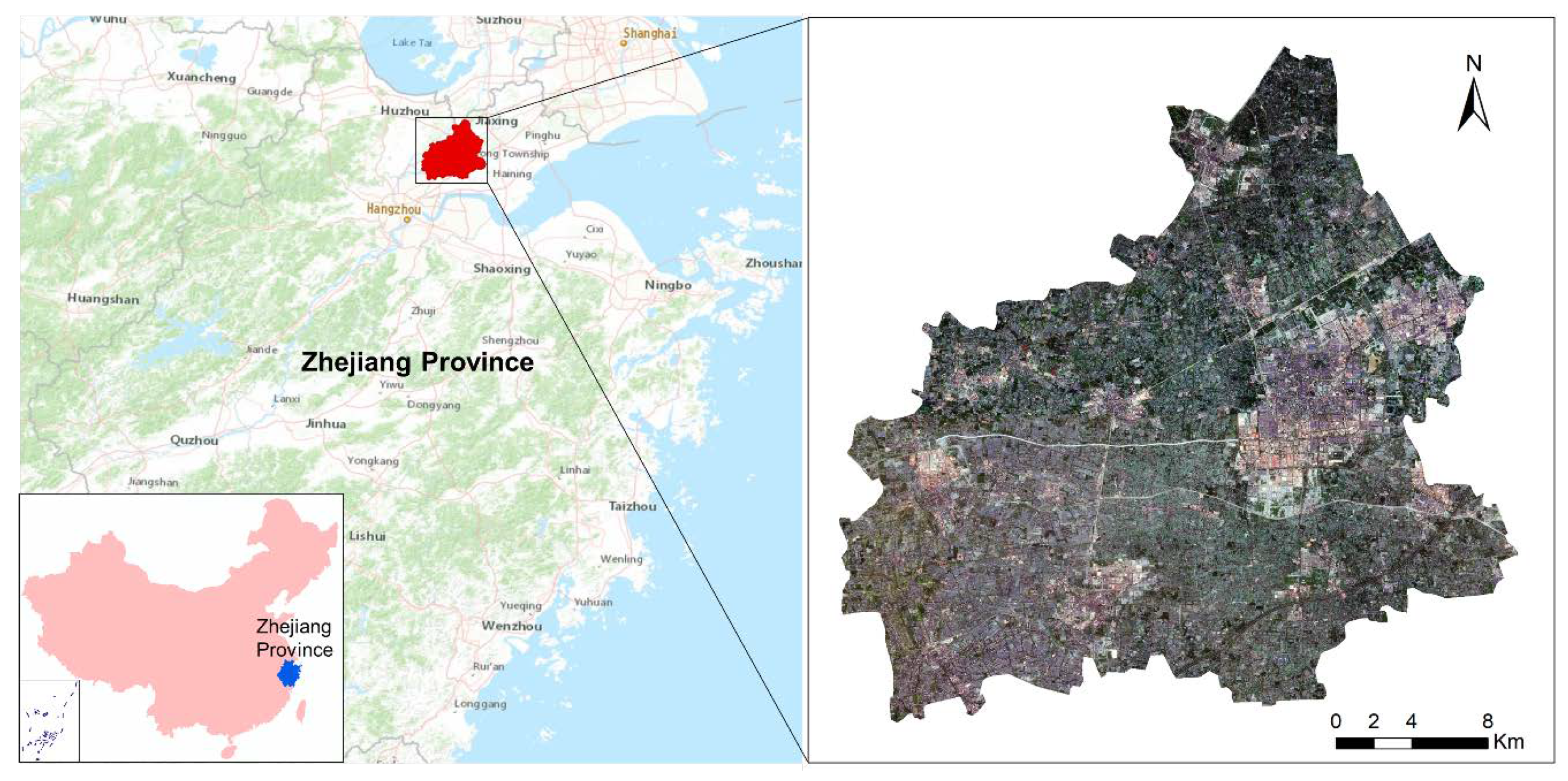
2.1.1. Study Area
2.1.2. Datasets and Preprocessing
Time Series SAR Data
Sentinel-2 Time Series Images
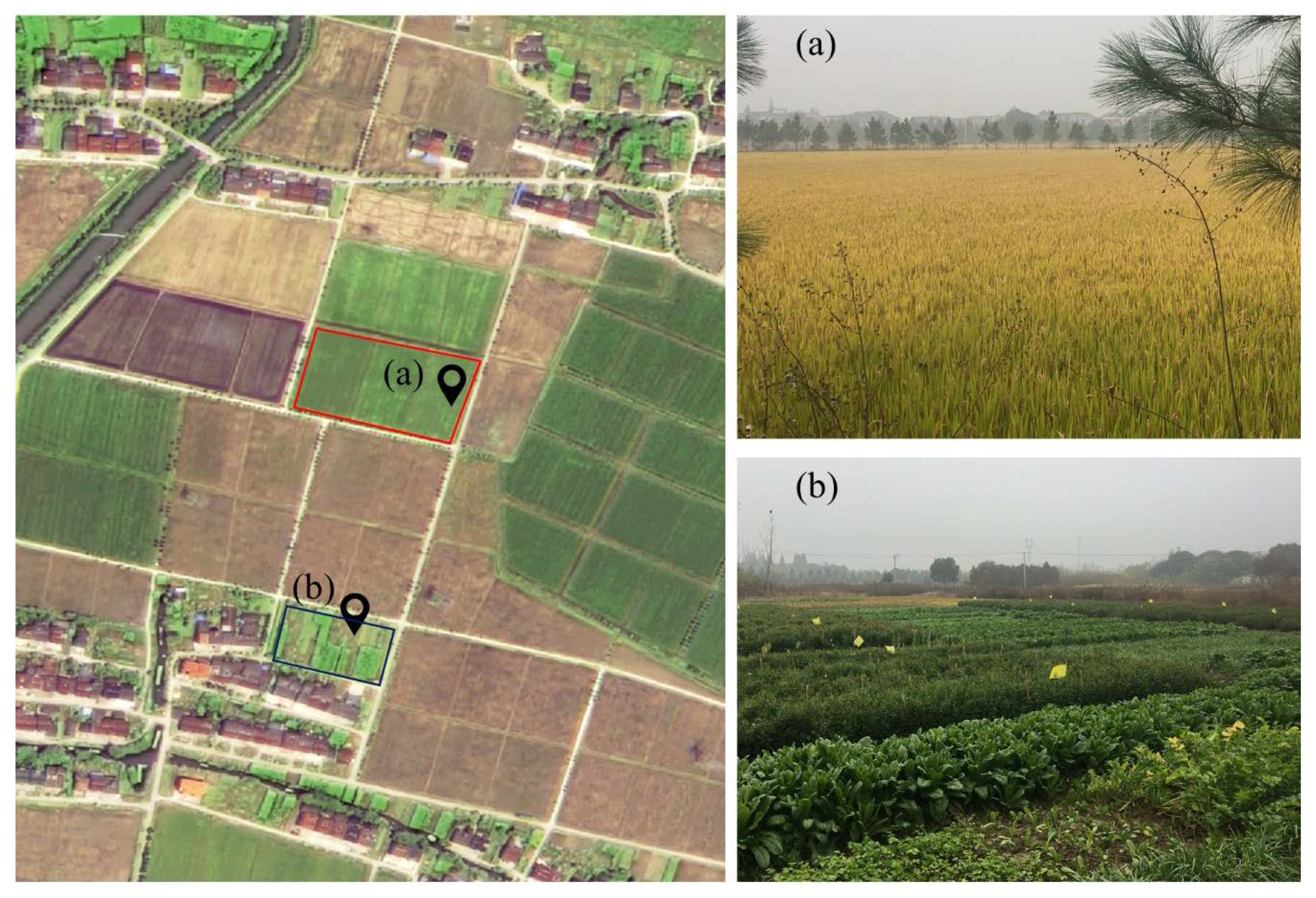
Field Sampling Data
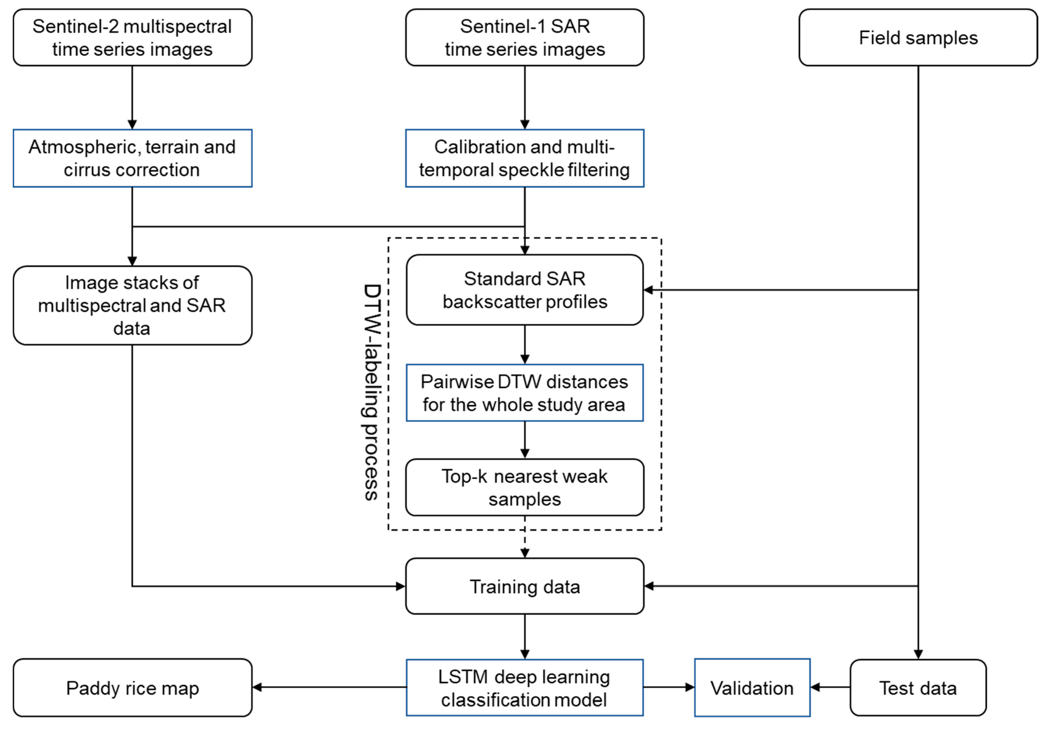
2.2. Methodology
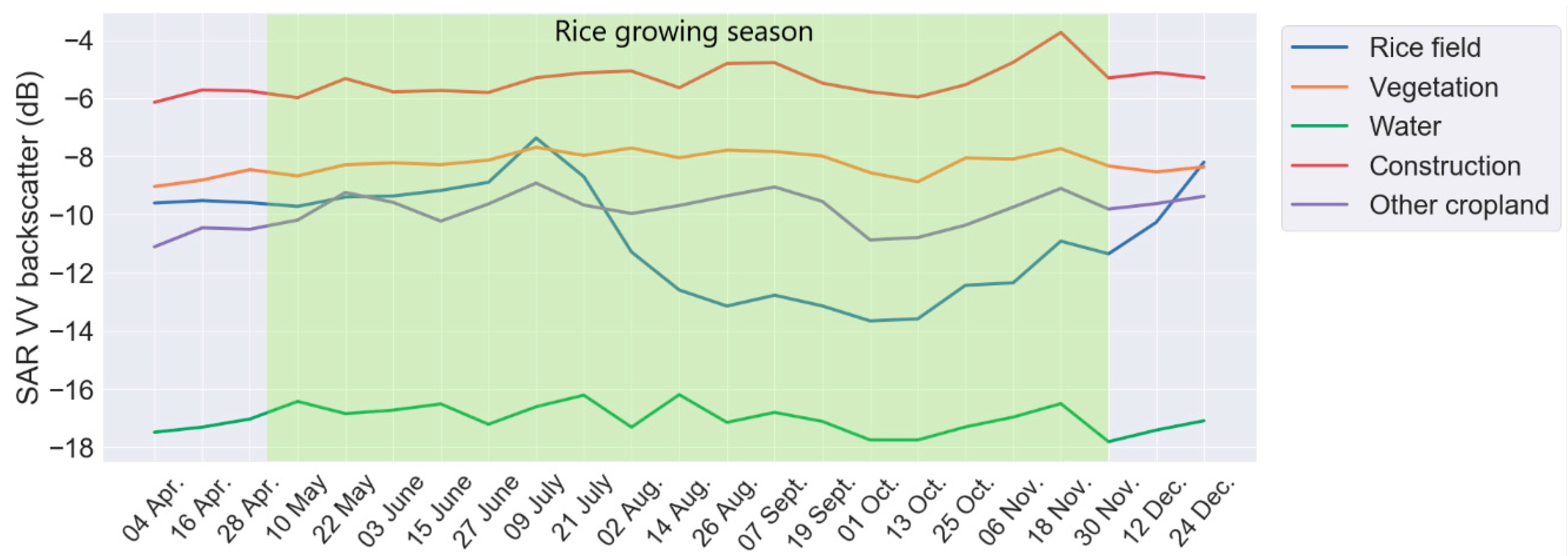
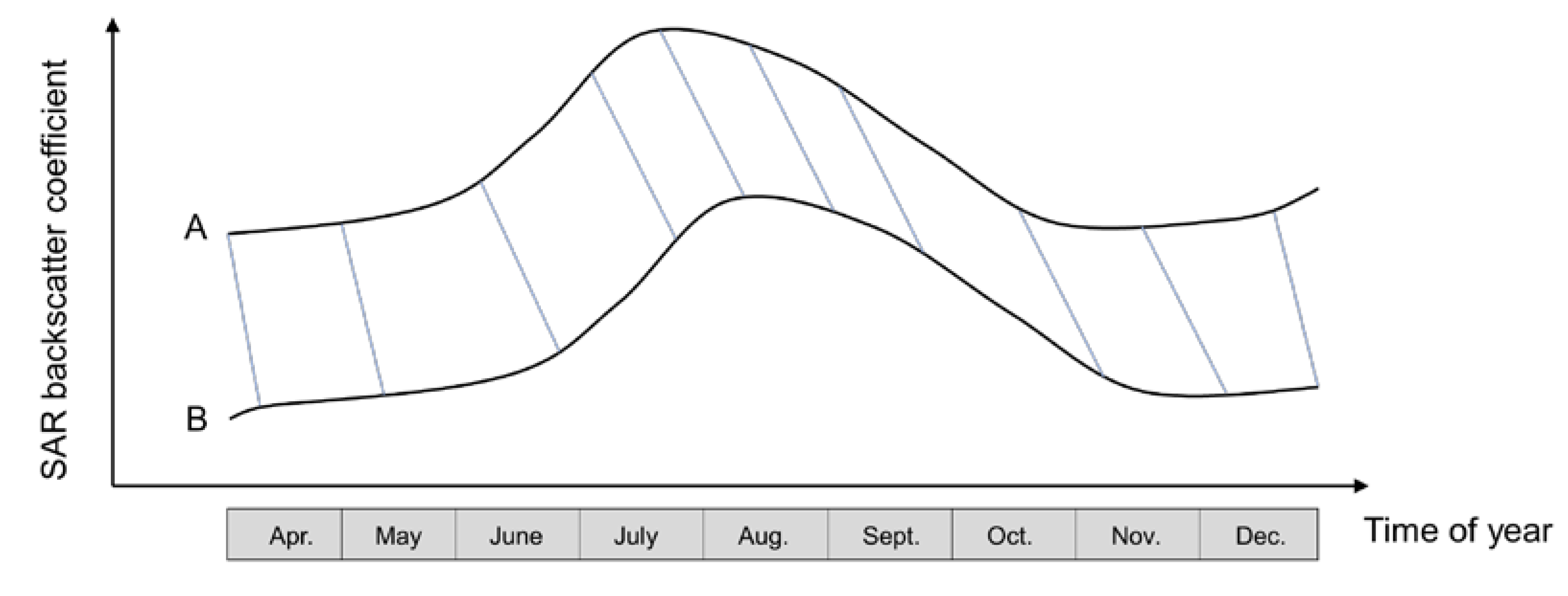
2.2.1. Standard Time Series SAR Backscatter Profiles
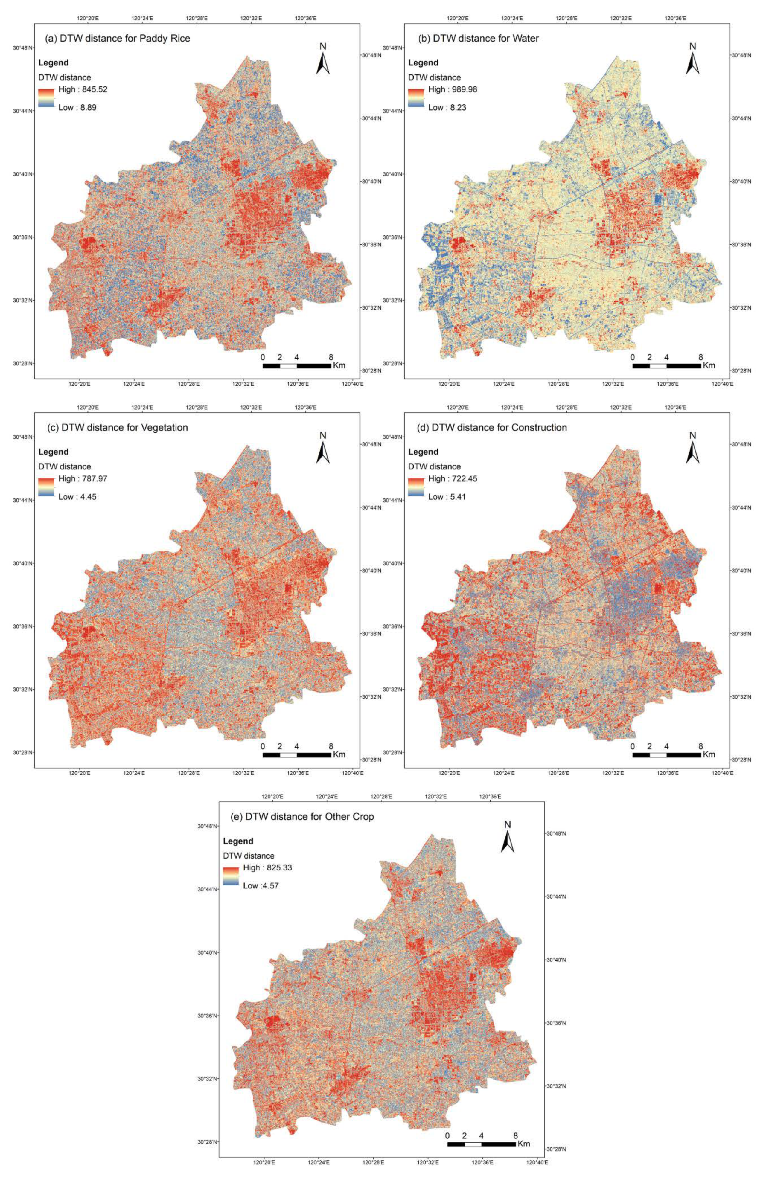
2.2.2. DTW Distance-Based Sampling
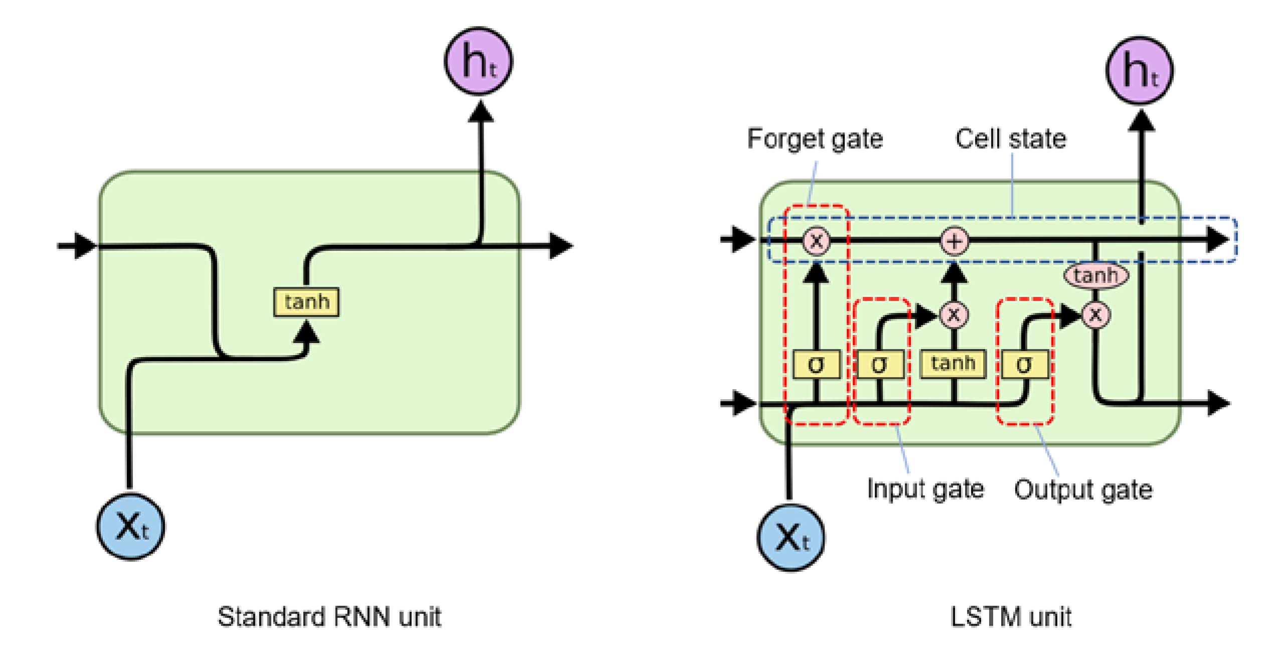
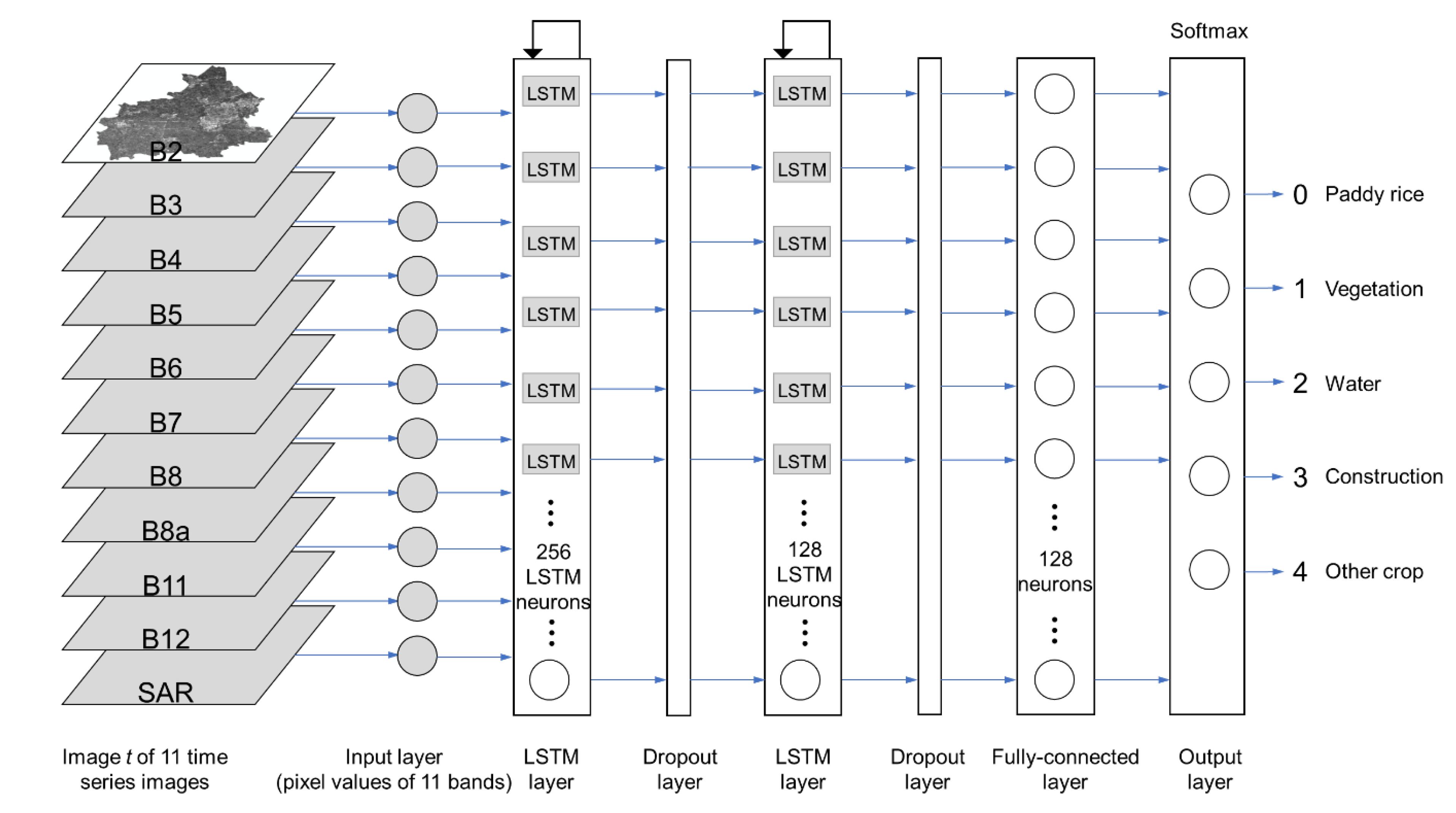
2.2.3. LSTM Deep Learning Classifier
2.2.4. Experiment Design
- Scheme 1: Supervised learning training on 10% of field samples compares with weakly supervised learning training on (10% of field samples + 5000 DTW-labeled samples for each land cover type).
- Scheme 2: Supervised learning training on 50% of field samples compares with weakly supervised learning training on (50% of field samples + 2000 DTW-labeled samples for each land cover type).
- Scheme 3: Supervised learning training on 80% of field samples compares with weakly supervised learning training on (80% of field samples + 2000 DTW-labeled samples for each land cover type).
3. Results
3.1. DTW Distance-Based Sampling Results
3.2. LSTM Classification Results
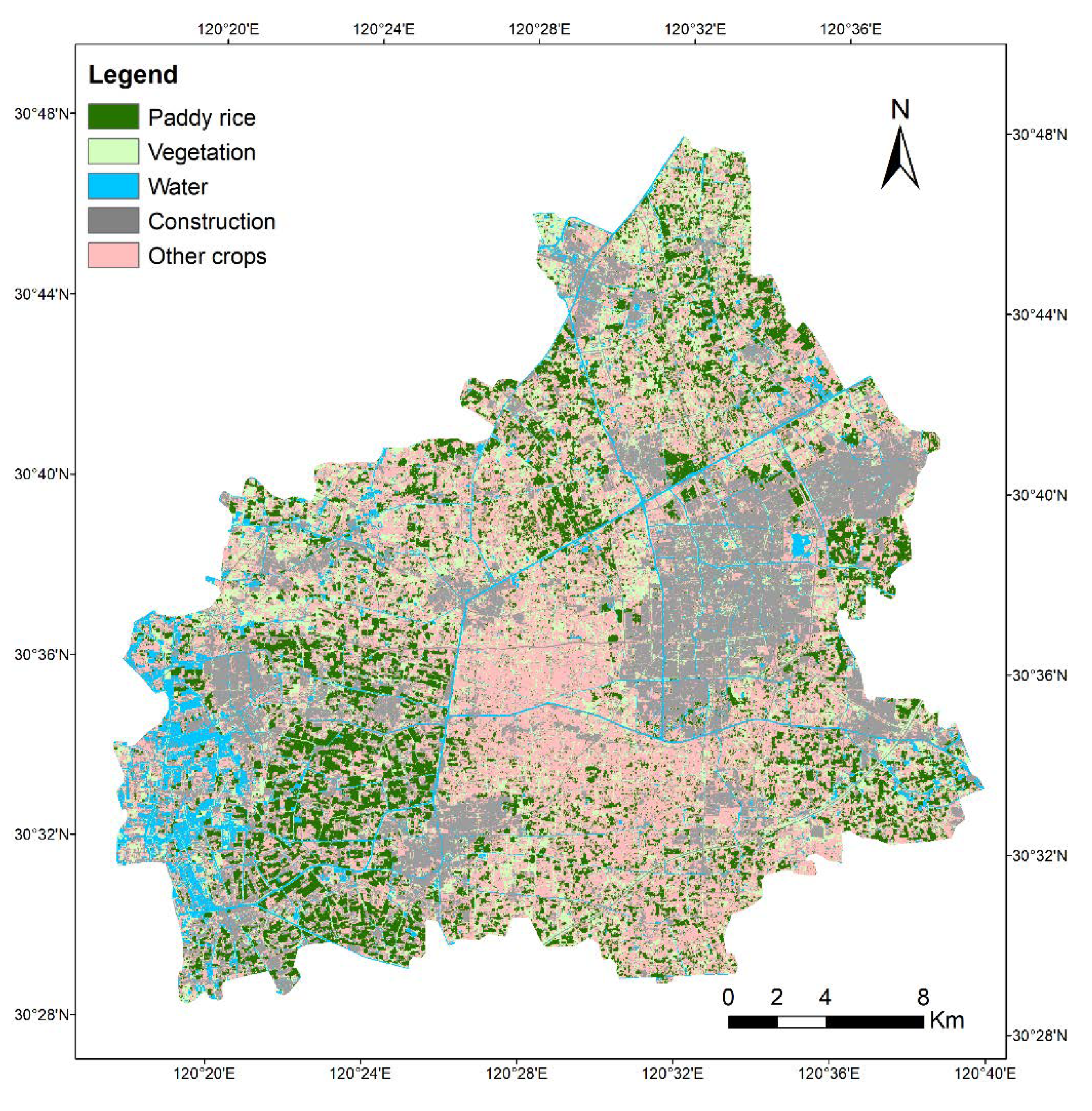
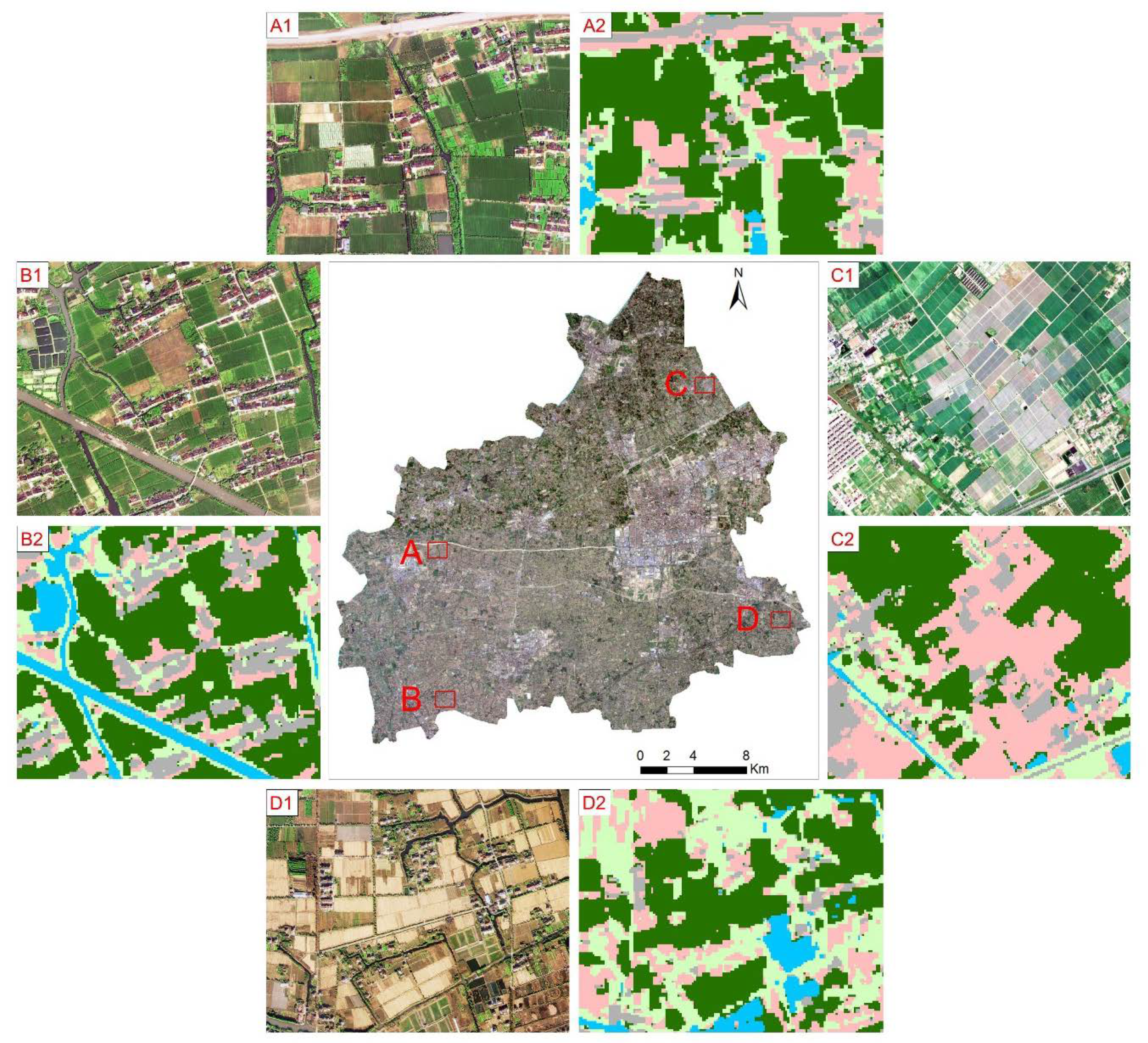
3.3. Paddy Rice Map
4. Discussion
5. Conclusions
Author Contributions
Funding
Conflicts of Interest
References
- Sarris, A. Rice in Global Markets. In Proceedings of the FAO Rice Conference 2004, Rome, Italy, 12–13 February 2004. [Google Scholar]
- Muthayya, S.; Sugimoto, J.D.; Montgomery, S.; Maberly, G.F. An overview of global rice production, supply, trade, and consumption. Ann. N. Y. Acad. Sci. 2014, 1324, 7–14. [Google Scholar] [CrossRef]
- Bouman, B. How much water does rice use. Management 2009, 69, 115–133. [Google Scholar]
- Dong, J.; Xiao, X. Evolution of regional to global paddy rice mapping methods: A review. ISPRS J. Photogramm. Remote Sens. 2016, 119, 214–227. [Google Scholar] [CrossRef] [Green Version]
- Jin, C.; Xiao, X.; Dong, J.; Qin, Y.; Wang, Z. Mapping paddy rice distribution using multi-temporal Landsat imagery in the Sanjiang Plain, northeast China. Front. Earth Sci. 2016, 10, 49–62. [Google Scholar] [CrossRef] [PubMed] [Green Version]
- Zhong, L.; Gong, P.; Biging, G.S. Efficient corn and soybean mapping with temporal extendability: A multi-year experiment using Landsat imagery. Remote Sens. Environ. 2014, 140, 1–13. [Google Scholar] [CrossRef]
- Xiao, X.; Boles, S.; Liu, J.; Zhuang, D.; Frolking, S.; Li, C.; Salas, W.; Moore, B., III. Mapping paddy rice agriculture in southern China using multi-temporal MODIS images. Remote Sens. Environ. 2005, 95, 480–492. [Google Scholar]
- Bazzi, H.; Baghdadi, N.; El Hajj, M.; Zribi, M.; Minh, D.H.T.; Ndikumana, E.; Courault, D.; Belhouchette, H. Mapping paddy rice using Sentinel-1 SAR time series in Camargue, France. Remote Sens. 2019, 11, 887. [Google Scholar] [CrossRef] [Green Version]
- Onojeghuo, A.O.; Blackburn, G.A.; Wang, Q.; Atkinson, P.M.; Kindred, D.; Miao, Y. Mapping paddy rice fields by applying machine learning algorithms to multi-temporal Sentinel-1A and Landsat data. Int. J. Remote Sens. 2018, 39, 1042–1067. [Google Scholar] [CrossRef] [Green Version]
- Xiao, X.; Boles, S.; Frolking, S.; Li, C.; Babu, J.Y.; Salas, W.; Moore, B., III. Mapping paddy rice agriculture in South and Southeast Asia using multi-temporal MODIS images. Remote Sens. Environ. 2006, 100, 95–113. [Google Scholar] [CrossRef]
- Yin, Q.; Liu, M.; Cheng, J.; Ke, Y.; Chen, X. Mapping Paddy Rice Planting Area in Northeastern China Using Spatiotemporal Data Fusion and Phenology-Based Method. Remote Sens. 2019, 11, 1699. [Google Scholar] [CrossRef] [Green Version]
- Torbick, N.; Salas, W.A.; Hagen, S.; Xiao, X. Monitoring rice agriculture in the Sacramento Valley, USA with multitemporal PALSAR and MODIS imagery. IEEE J. Sel. Top. Appl. Earth Obs. Remote Sens. 2010, 4, 451–457. [Google Scholar] [CrossRef]
- Zhang, Y.; Wang, C.; Wu, J.; Qi, J.; Salas, W.A. Mapping paddy rice with multitemporal ALOS/PALSAR imagery in southeast China. Int. J. Remote Sens. 2009, 30, 6301–6315. [Google Scholar] [CrossRef]
- Aschbacher, J.; Pongsrihadulchai, A.; Karnchanasutham, S.; Rodprom, C.; Paudyal, D.; Le Toan, T. Assessment of ERS-1 SAR data for rice crop mapping and monitoring. In Proceedings of the 1995 International Geoscience and Remote Sensing Symposium, IGARSS’95, Florence, Italy, 10–14 July 1995; pp. 2183–2185. [Google Scholar]
- Wu, F.; Wang, C.; Zhang, H.; Zhang, B.; Tang, Y. Rice crop monitoring in South China with RADARSAT-2 quad-polarization SAR data. IEEE Geosci. Remote Sens. Lett. 2010, 8, 196–200. [Google Scholar] [CrossRef]
- Clauss, K.; Ottinger, M.; Künzer, C. Mapping rice areas with Sentinel-1 time series and superpixel segmentation. Int. J. Remote Sens. 2018, 39, 1399–1420. [Google Scholar] [CrossRef] [Green Version]
- Nguyen, D.B.; Gruber, A.; Wagner, W. Mapping rice extent and cropping scheme in the Mekong Delta using Sentinel-1A data. Remote Sens. Lett. 2016, 7, 1209–1218. [Google Scholar] [CrossRef]
- Le Toan, T.; Ribbes, F.; Wang, L.-F.; Floury, N.; Ding, K.-H.; Kong, J.A.; Fujita, M.; Kurosu, T. Rice crop mapping and monitoring using ERS-1 data based on experiment and modeling results. IEEE Trans. Geosci. Remote Sens. 1997, 35, 41–56. [Google Scholar] [CrossRef]
- Guan, X.; Huang, C.; Liu, G.; Meng, X.; Liu, Q. Mapping rice cropping systems in Vietnam using an NDVI-based time-series similarity measurement based on DTW distance. Remote Sens. 2016, 8, 19. [Google Scholar] [CrossRef] [Green Version]
- Belgiu, M.; Csillik, O. Sentinel-2 cropland mapping using pixel-based and object-based time-weighted dynamic time warping analysis. Remote Sens. Environ. 2018, 204, 509–523. [Google Scholar] [CrossRef]
- Guan, X.; Liu, G.; Huang, C.; Meng, X.; Liu, Q.; Wu, C.; Ablat, X.; Chen, Z.; Wang, Q. An Open-Boundary Locally Weighted Dynamic Time Warping Method for Cropland Mapping. Isprs Int. J. Geo-Inf. 2018, 7, 75. [Google Scholar] [CrossRef] [Green Version]
- Li, M.; Bijker, W. Vegetable classification in Indonesia using Dynamic Time Warping of Sentinel-1A dual polarization SAR time series. Int. J. Appl. Earth Obs. Geoinf. 2019, 78, 268–280. [Google Scholar] [CrossRef]
- Chen, C.-F.; Son, N.-T.; Chen, C.-R.; Chang, L.-Y. Wavelet filtering of time-series moderate resolution imaging spectroradiometer data for rice crop mapping using support vector machines and maximum likelihood classifier. J. Appl. Remote Sens. 2011, 5, 053525. [Google Scholar] [CrossRef]
- McCloy, K.; Smith, F.; Robinson, M. Monitoring rice areas using Landsat MSS data. Int. J. Remote Sens. 1987, 8, 741–749. [Google Scholar] [CrossRef]
- Clauss, K.; Yan, H.; Kuenzer, C. Mapping paddy rice in China in 2002, 2005, 2010 and 2014 with MODIS time series. Remote Sens. 2016, 8, 434. [Google Scholar] [CrossRef] [Green Version]
- Kücük, C.; Taskın, G.; Erten, E. Paddy-rice phenology classification based on machine-learning methods using multitemporal co-polar X-band SAR images. IEEE J. Sel. Top. Appl. Earth Obs. Remote Sens. 2016, 9, 2509–2519. [Google Scholar] [CrossRef]
- Park, S.; Im, J.; Park, S.; Yoo, C.; Han, H.; Rhee, J. Classification and mapping of paddy rice by combining Landsat and SAR time series data. Remote Sens. 2018, 10, 447. [Google Scholar] [CrossRef] [Green Version]
- Teluguntla, P.; Thenkabail, P.S.; Oliphant, A.; Xiong, J.; Gumma, M.K.; Congalton, R.G.; Yadav, K.; Huete, A. A 30-m Landsat-derived cropland extent product of Australia and China using random forest machine learning algorithm on Google Earth Engine cloud computing platform. ISPRS J. Photogramm. Remote Sens. 2018, 144, 325–340. [Google Scholar] [CrossRef]
- Gumma, M.K.; Nelson, A.; Thenkabail, P.S.; Singh, A.N. Mapping rice areas of South Asia using MODIS multitemporal data. J. Appl. Remote Sens. 2011, 5, 053547. [Google Scholar] [CrossRef] [Green Version]
- Wang, J.; Yang, Y.; Mao, J.; Huang, Z.; Huang, C.; Xu, W. CNN-RNN: A unified framework for multi-label image classification. In Proceedings of the IEEE Conference on Computer Vision and Pattern Recognition, Las Vegas, NV, USA, 26–30 June 2016; pp. 2285–2294. [Google Scholar]
- Kussul, N.; Lavreniuk, M.; Skakun, S.; Shelestov, A. Deep learning classification of land cover and crop types using remote sensing data. IEEE Geosci. Remote Sens. Lett. 2017, 14, 778–782. [Google Scholar] [CrossRef]
- Zhang, M.; Lin, H.; Wang, G.; Sun, H.; Fu, J. Mapping paddy rice using a convolutional neural network (CNN) with Landsat 8 datasets in the Dongting Lake Area, China. Remote Sens. 2018, 10, 1840. [Google Scholar] [CrossRef] [Green Version]
- Sun, Z.; Di, L.; Fang, H. Using long short-term memory recurrent neural network in land cover classification on Landsat and Cropland data layer time series. Int. J. Remote Sens. 2019, 40, 593–614. [Google Scholar] [CrossRef]
- Clement, M.; Kilsby, C.; Moore, P. Multi-temporal synthetic aperture radar flood mapping using change detection. J. Flood Risk Manag. 2018, 11, 152–168. [Google Scholar] [CrossRef]
- Cai, Y.; Guan, K.; Peng, J.; Wang, S.; Seifert, C.; Wardlow, B.; Li, Z. A high-performance and in-season classification system of field-level crop types using time-series Landsat data and a machine learning approach. Remote Sens. Environ. 2018, 210, 35–47. [Google Scholar] [CrossRef]
- Sakoe, H.; Chiba, S. Dynamic programming algorithm optimization for spoken word recognition. IEEE Trans. Acoust. SpeechSignal Process. 1978, 26, 43–49. [Google Scholar] [CrossRef] [Green Version]
- Maus, V.; Câmara, G.; Cartaxo, R.; Sanchez, A.; Ramos, F.M.; De Queiroz, G.R. A time-weighted dynamic time warping method for land-use and land-cover mapping. IEEE J. Sel. Top. Appl. Earth Obs. Remote Sens. 2016, 9, 3729–3739. [Google Scholar] [CrossRef]
- Petitjean, F.; Inglada, J.; Gancarski, P. Satellite image time series analysis under time warping. IEEE Trans. Geosci. Remote Sens. 2012, 50, 3081–3095. [Google Scholar] [CrossRef]
- Berndt, D.J.; Clifford, J. Using dynamic time warping to find patterns in time series. In Proceedings of the KDD Workshop, Seattle, WA, USA, 31 July 1994; pp. 359–370. [Google Scholar]
- Hochreiter, S.; Schmidhuber, J. Long short-term memory. Neural Comput. 1997, 9, 1735–1780. [Google Scholar] [CrossRef] [PubMed]
- Understanding LSTM Networks. Available online: https://colah.github.io/posts/2015-08-Understanding-LSTMs (accessed on 16 June 2020).
- Goodfellow, I.; Bengio, Y.; Courville, A.; Bengio, Y. Deep Learning. MIT press Cambridge: Cambridge, MA, USA, 2016; pp. 226–227. [Google Scholar]
- Zhong, L.; Hu, L.; Zhou, H. Deep learning based multi-temporal crop classification. Remote Sens. Environ. 2019, 221, 430–443. [Google Scholar] [CrossRef]
- Qiu, B.; Li, W.; Tang, Z.; Chen, C.; Qi, W. Mapping paddy rice areas based on vegetation phenology and surface moisture conditions. Ecol. Indic. 2015, 56, 79–86. [Google Scholar] [CrossRef]
- Zhang, G.; Xiao, X.; Dong, J.; Kou, W.; Jin, C.; Qin, Y.; Zhou, Y.; Wang, J.; Menarguez, M.A.; Biradar, C. Mapping paddy rice planting areas through time series analysis of MODIS land surface temperature and vegetation index data. Isprs J. Photogramm. Remote Sens. 2015, 106, 157–171. [Google Scholar] [CrossRef] [Green Version]
- Xiao, X.; Boles, S.; Frolking, S.; Salas, W.; Moore, B., III; Li, C.; He, L.; Zhao, R. Observation of flooding and rice transplanting of paddy rice fields at the site to landscape scales in China using VEGETATION sensor data. Int. J. Remote Sens. 2002, 23, 3009–3022. [Google Scholar] [CrossRef]
- Chen, C.; McNairn, H. A neural network integrated approach for rice crop monitoring. Int. J. Remote Sens. 2006, 27, 1367–1393. [Google Scholar] [CrossRef]


| SAR Images | |
|---|---|
| Sensor | Sentinel-1A |
| Data level | Level-1 ground range detected |
| Spatial resolution | 10 m |
| Wavelength | C band |
| Polarization | VV |
| Pass | Ascending |
| Acquisition mode | IW |
| Acquisition date (23 successive images with 12-day interval) | 4 April 2018 |
| 16 April 2018 | |
| 28 April 2018 | |
| …… 24 December 2018 | |
| Multispectral Optical Images | |
|---|---|
| Sensor | Sentinel-2A, Sentinel-2B |
| Data level | Level-1C |
| Spatial resolution | 10 m, 20 m |
| Band | B2, B3, B4, B5, B6, B7, B8, B8a, B11, B12 |
| Acquisition date (11 images) | 9 April 2018 |
| 19 April 2018 | |
| 4 May 2018 | |
| 9 May 2018 | |
| 18 June 2018 | |
| 18 July 2018 | |
| 23 July 2018 | |
| 28 July 2018 | |
| 7 August 2018 | |
| 1 October 2018 | |
| 10 November 2018 | |
| Learning Rate | Dropout Rate | Batch Size | Loss Function | Optimizer |
|---|---|---|---|---|
| 0.001 | 0.5 | 64 | Categorical cross-entropy | Adam algorithm |
| Experiment | OA | Paddy Rice PA | Paddy Rice UA | Paddy Rice Support | Kappa | |
|---|---|---|---|---|---|---|
| Scheme 1 | Supervised | 0.937 | 0.904 | 0.917 | 2281 | 0.921 |
| Weakly supervised | 0.854 | 0.981 | 0.961 | 2281 | 0.817 | |
| Scheme 2 | Supervised | 0.973 | 0.968 | 0.972 | 2281 | 0.966 |
| Weakly supervised | 0.986 | 0.985 | 0.993 | 2281 | 0.982 | |
| Scheme 3 | Supervised | 0.982 | 0.988 | 0.987 | 913 | 0.978 |
| Weakly supervised | 0.989 | 0.996 | 0.984 | 913 | 0.986 | |
| Paddy Rice | Vegetation | Water | Construction | Other Crops | |
|---|---|---|---|---|---|
| Paddy rice | 2092 | 54 | 0 | 23 | 112 |
| Vegetation | 42 | 2276 | 3 | 4 | 66 |
| Water | 5 | 0 | 2118 | 24 | 0 |
| Construction | 3 | 0 | 21 | 3015 | 2 |
| Other crops | 173 | 158 | 7 | 72 | 1885 |
| PA | 0.904 | 0.915 | 0.986 | 0.961 | 0.913 |
| UA | 0.917 | 0.948 | 0.986 | 0.99 | 0.821 |
| OA | 0.937 | ||||
| Kappa | 0.921 | ||||
| Paddy Rice | Vegetation | Water | Construction | Other Crops | |
|---|---|---|---|---|---|
| Paddy rice | 2193 | 12 | 0 | 6 | 70 |
| Vegetation | 6 | 2066 | 0 | 58 | 261 |
| Water | 6 | 0 | 2091 | 16 | 34 |
| Construction | 0 | 50 | 2 | 2742 | 247 |
| Other crops | 30 | 775 | 39 | 163 | 1288 |
| PA | 0.981 | 0.712 | 0.981 | 0.919 | 0.678 |
| UA | 0.961 | 0.864 | 0.974 | 0.902 | 0.561 |
| OA | 0.854 | ||||
| Kappa | 0.817 | ||||
Publisher’s Note: MDPI stays neutral with regard to jurisdictional claims in published maps and institutional affiliations. |
© 2020 by the authors. Licensee MDPI, Basel, Switzerland. This article is an open access article distributed under the terms and conditions of the Creative Commons Attribution (CC BY) license (http://creativecommons.org/licenses/by/4.0/).
Share and Cite
Wang, M.; Wang, J.; Chen, L. Mapping Paddy Rice Using Weakly Supervised Long Short-Term Memory Network with Time Series Sentinel Optical and SAR Images. Agriculture 2020, 10, 483. https://doi.org/10.3390/agriculture10100483
Wang M, Wang J, Chen L. Mapping Paddy Rice Using Weakly Supervised Long Short-Term Memory Network with Time Series Sentinel Optical and SAR Images. Agriculture. 2020; 10(10):483. https://doi.org/10.3390/agriculture10100483
Chicago/Turabian StyleWang, Mo, Jing Wang, and Li Chen. 2020. "Mapping Paddy Rice Using Weakly Supervised Long Short-Term Memory Network with Time Series Sentinel Optical and SAR Images" Agriculture 10, no. 10: 483. https://doi.org/10.3390/agriculture10100483