Time Series Prediction with Artificial Neural Networks: An Analysis Using Brazilian Soybean Production

Abstract

Food production to meet human demand has been a challenge to society. Nowadays, one of the main sources of feeding is soybean. Considering agriculture food crops, soybean is sixth by production volume and the fourth by both production area and economic value. The grain can be used directly to human consumption, but it is highly used as a source of protein for animal production that corresponds 75% of the total, or as oil and derived food products. Brazil and the US are the most important players responsible for more than 70% of world production. Therefore, a reliable forecasting is essential for decision-makers to plan adequate policies to this important commodity and to establish the necessary logistical resources. In this sense, this study aims to predict soybean harvest area, yield, and production using Artificial Neural Networks (ANN) and compare with classical methods of Time Series Analysis. To this end, we collected data from a time series (1961–2016) regarding soybean production in Brazil. The results reveal that ANN is the best approach to predict soybean harvest area and production while classical linear function remains more effective to predict soybean yield. Moreover, ANN presents as a reliable model to predict time series and can help the stakeholders to anticipate the world soybean offer.

1. Introduction

World’s population is projected to reach 9.8 billion in 2050 [1] and food production needs to increase by 60% to meet the demand [2,3]. One reason for that is the developing countries—that have been growing much more rapidly than the industrial countries—are creating implications for world food demand mainly in products such as animal-based, fruits, and vegetables [4]. However, declining rates of growth in crop yields, slowing investment in agricultural research, and rising commodity prices have raised concerns of a general slowdown in global agricultural harvest area, yield, and production [5].

The rapid per capita income growth in countries like China and India (40% world population) pressure food supply chains shifting towards animal-based products that require disproportionately more agricultural resources in production [4,6] such as land, water, and vegetable protein [7]. Moreover, there is a concern revolving around big agriculture growers such as Brazil and the US using their agriculture areas to produce biofuels [6].

It is not only in the economy that this relationship between food demand and income are finding shelter. It is possible to verify in the literature a connection about technology and agricultural production. Crop yield and production, for instance, have been studied in the light of artificial intelligence. Khan et al. [8] predicted fruit production using deep neural networks. García-Martiínez et al. [9] estimated corn grain yield with a neural network using multispectral and RGB images acquired with unmanned aerial vehicles. Maimaitijiang et al. [10] predicted soybean yield using multimodal data fusion and deep learning. These applications are a clear attempt to improve knowledge about food production and provide decision-makers with valuable information to face the challenges of food demand.

Another possible solution discussed is the use of areas in Latin America and the Caribbean to expand agriculture production [11]. Brazil, for instance, has more than 8 million ${\mathrm{km}}^2$ of area and uses only 15% of its arable land—approximately 60 of 400 million hectares [12]. The country is an important global food supplier, and it is estimated that one out of four agribusiness products in circulation around the world came from Brazil [13]. Despite the concern of biofuel production, sugarcane occupies only 8.9 million hectares of arable land [14], and the majority is used for sugar production rather than ethanol.

Brazil has more than 300 different crops and exports 350 types of products to 180 countries. The main export products are sugar, coffee, maize, orange juice, cotton, and soybean. Among these products, soybean is the main global source of protein, and the country is the major exporter that corresponded for approximately 29.9% of agribusiness external sales in 2016—USD 25.4 billion [13]. According to the Department of Agriculture of United States—USDA [15], Brazilian exports of the soybean complex are 81% grains, 15.7% meal, and 3.3% refined oil.

Soybean production has overspread inside the country from south, through the center-western to the northeast area. These movements are motivated by low land cost, and investments in agriculture inputs, mechanization, and infrastructure [16,17,18]. Other factors contributing to soybean growth in Brazil include the genetic improvement of seeds, increasingly productive planting systems [19], favourable climatic conditions, predictable precipitation patterns, and public financing policies for soybean plantations [20].

The soybean production is evaluated considering three categories: harvest area, yield, and production. The two main players are Brazil and the US, the former planted a harvest area of 36.9 million of hectares that produced 120.9 million of tones with a yield of 3.3 tones per hectare [21] and the latter planted a harvest area around 30.8 million of hectares with a production of 96.8 million tons and a yield of 3.1 tones per hectare [22]. These values are constantly predicted using classical methods and presented to stakeholders by government agencies. However, the respective literature is sparse and relates to agronomy aspects of soybean yield [10,23,24]. In this paper, we focus on the prediction of these soybean indicators based on the previous crop data.

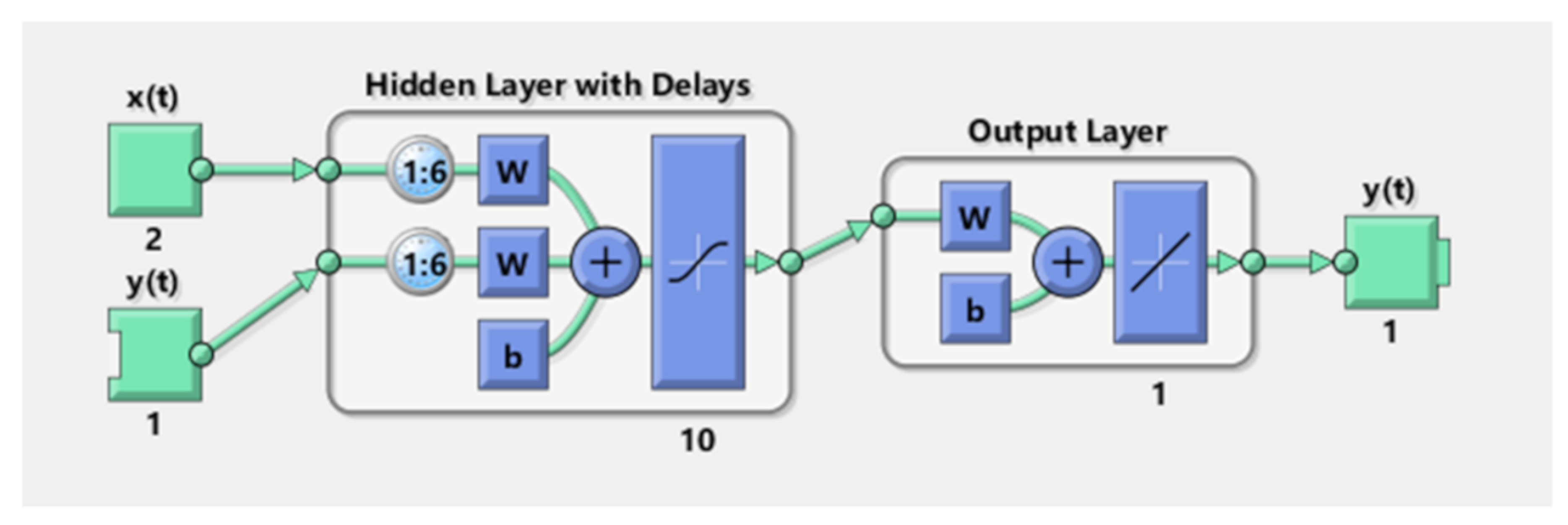
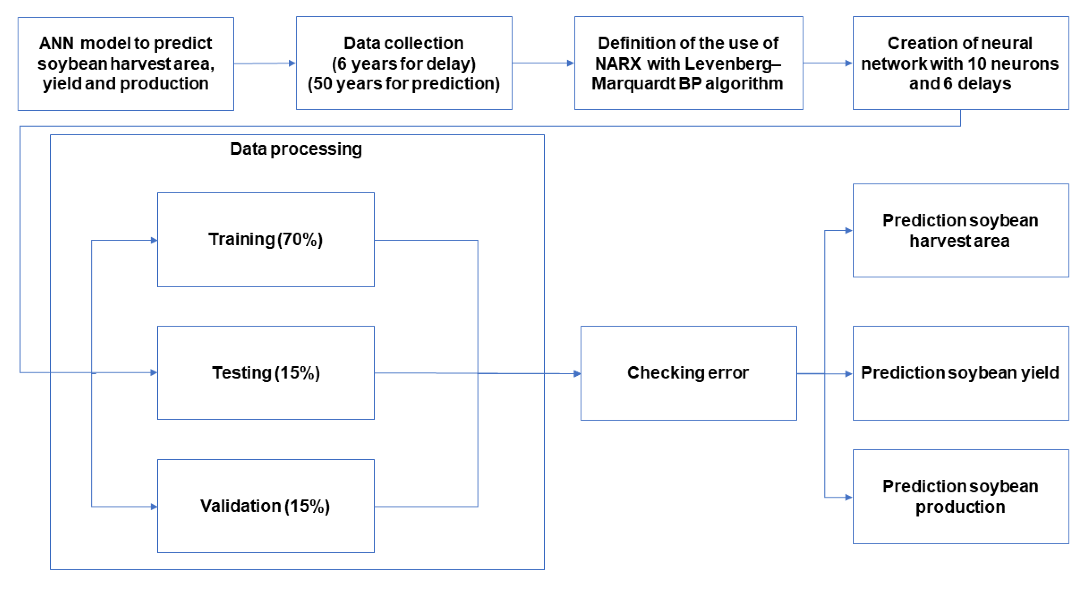
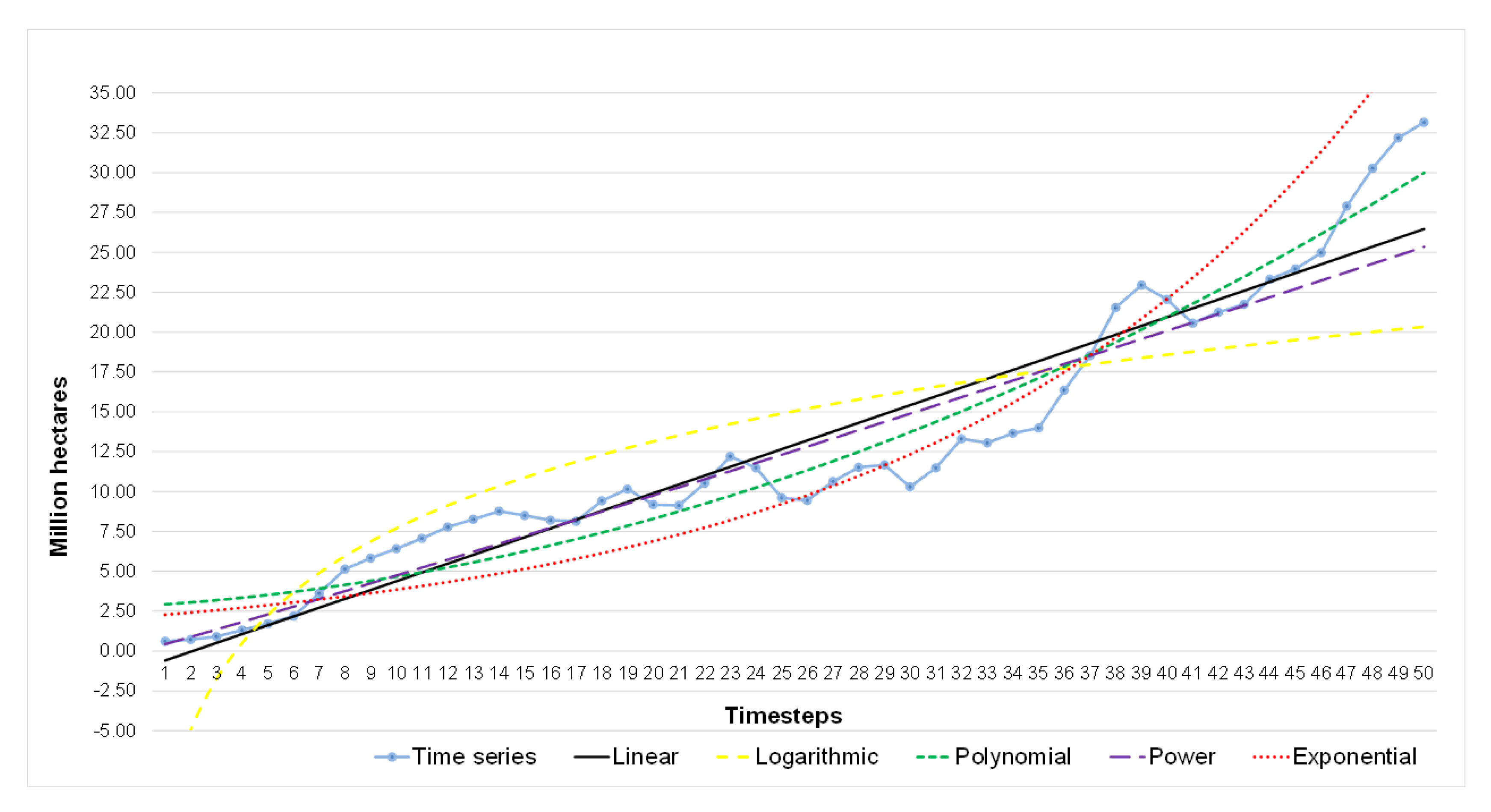
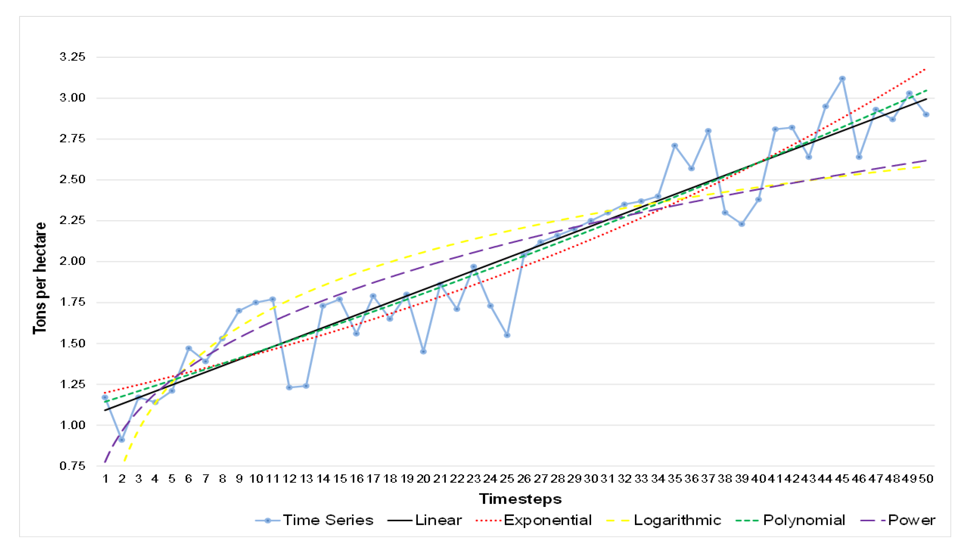
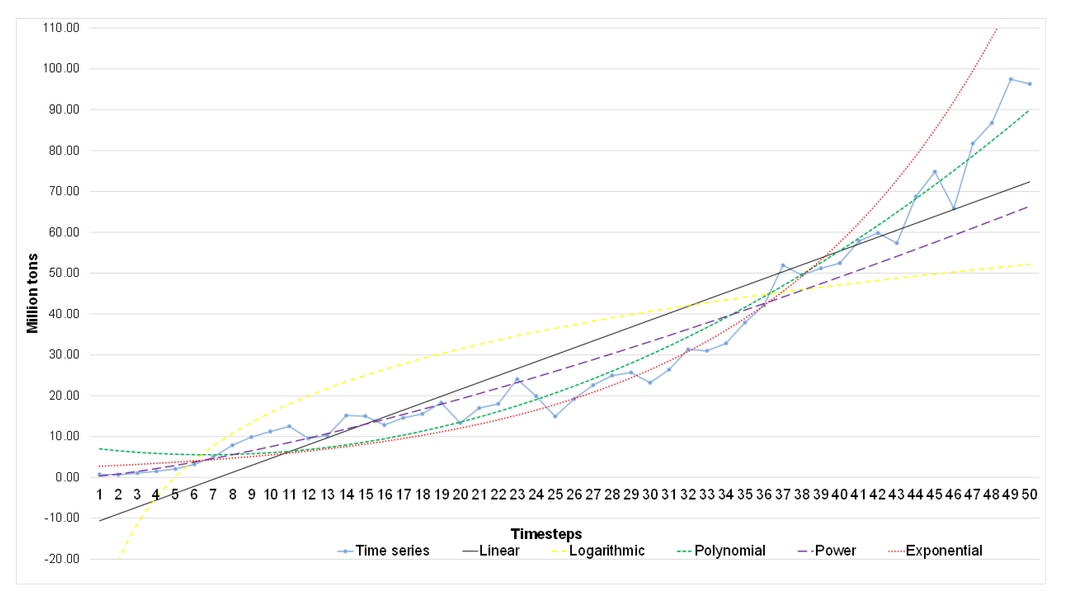
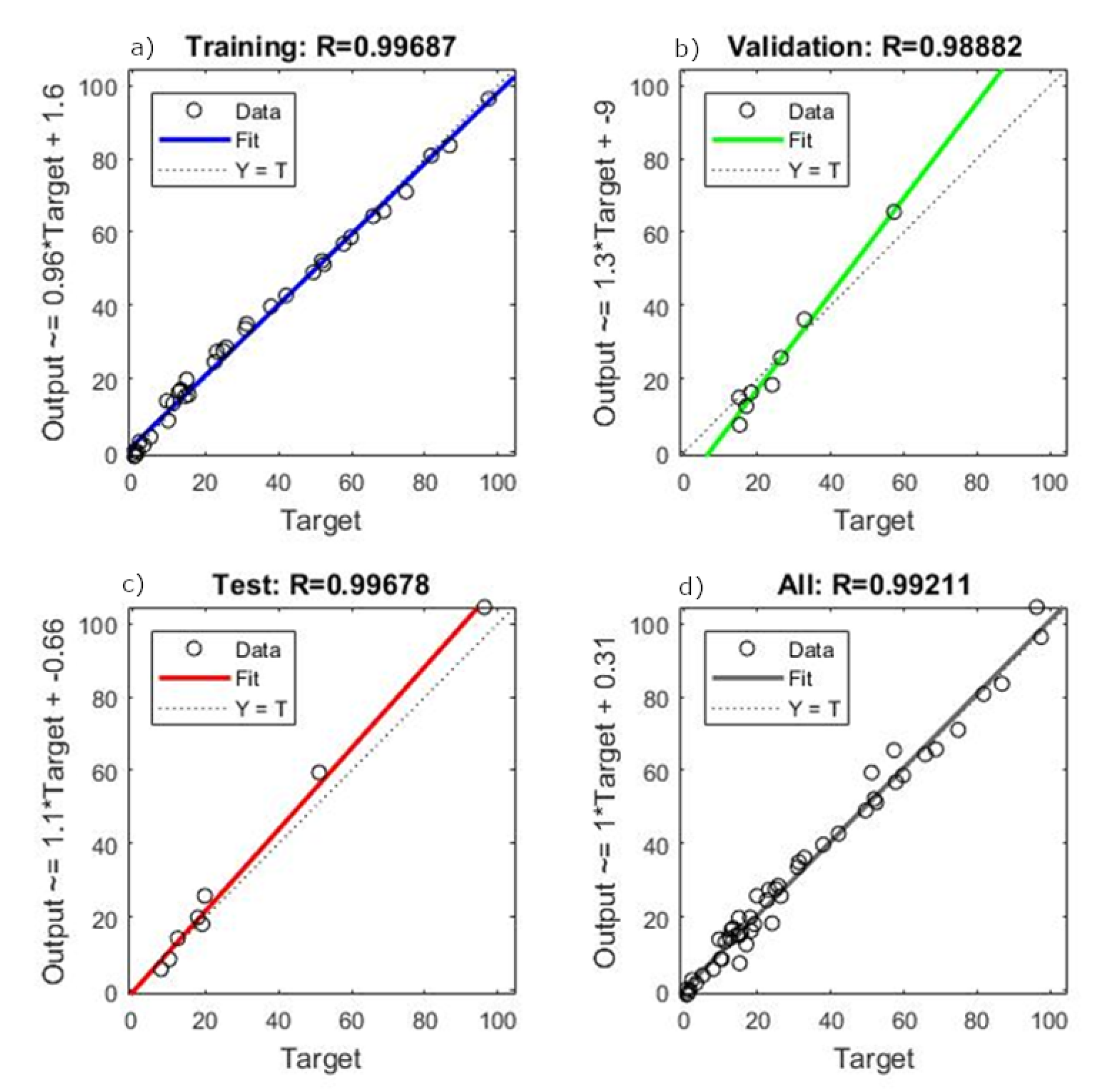
Therefore, our study aims to estimate Brazilian soybean harvest area, yield, and production adopting Artificial Neural Networks (ANN) and comparing with classical methods of Time Series Analysis. To this end, we collected the values of harvest area, production, and yield over a period of 56 years (1961–2016). We established the trend lines for five functions: Linear, Exponential, Logarithmic, Polynomial, and Power, and compared these results with an ANN model with 10 neurons and six delays computed using a Nonlinear Autoregressive Network with External Input-NARX with Levenberg—Marquardt backpropagation for training the network.

The results show that the ANN model is the most efficient method to predict soybean harvest area and production. The novelty of this paper is to obtain a reliable prediction for soybean production measures using an ANN model and dealing with a short data period time series (50 years) [25]. The period of 1961–1966 was used only for ANN model delay.

This paper is divided into sections: Section 1 presents this introduction and literature review, Section 2 shows the methodological procedures, Section 3 deal with results and discussion, and Section 4 presents the conclusions of the study.

1.1. Artificial Neural Networks

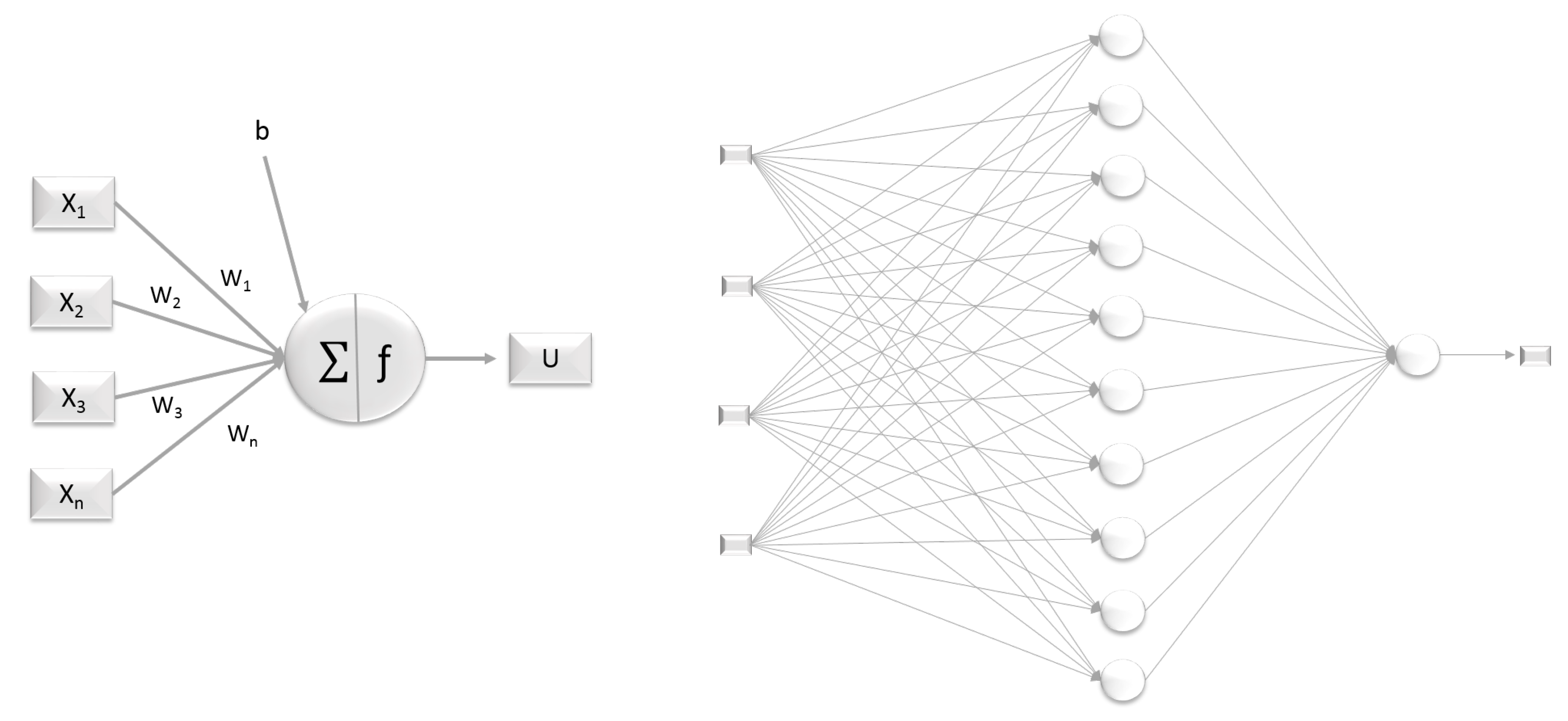
Artificial Neural Networks, as the name proposed, use artificial neurons connected in layers to simulate human synapse (Figure 1). A mathematical model mimics the neural structure to learn and to acquire knowledge via experiences (Equations (1) and (2)). This technology is effective to solve problems—dynamic and nonlinear—such as pattern recognition and prediction [25,26,27,28,29,30].

$$ne=\sum _{i=1}^n{x}_i{w}_i+b_i$$

(1)

$$u=f\left(ne\right)$$

(2)

where $x_1\dots x_n$ are the input values (data set), $w_1\dots w_n$ are the weights, and b is the activation threshold (bias) in the neuron potential $ne$ [25,26,31].

Among several types of neuron activation functions, the most common are: hyperbolic tangent (Equation (3)), hidden layer, and linear. The last one always assumes values identical to the activation potential n [25,26,31]:

$$f\left(ne\right)=\frac{1-e^{-\beta u}}{1+e^{-\beta u}}$$

(3)

where $\beta$ is the constant associated with the slope of the hyperbolic tangent function and the output values assume numbers between −1 and 1.

ANN uses previous data for training the network and minimizes errors between the insertion and the estimation. This process adjusts the weights and possible bias for each neuron interaction. The training usually stops when finding out the optimal learning rate [25,26,27,28,29,30].

There are various ANN techniques such as General Regression Neural Network (GRNN), Backpropagation Neural Network (BNN), Radial Base Function Neural Network (RBFNN), and Adaptive Neuro-Fuzzy Inference System (ANFIS) [32]. Backpropagation (BP) is a learning algorithm widely used in forecasting problems with ANN, and the networks [30]. The weights between the different layers may be updated using the BP algorithm, with momentum and learning rate. Moreover, the weights between the different layers may be updated where the error is then propagated backward from the output to the input layer [33].

Some studies have been using ANN to study the agricultural environment. Garg et al. [30] compare the performance between different training methods using an ANN model to forecast wheat production in India. The data contain 95 years of wheat production (1919–2013), and the results revealed that the algorithms most effective in training methods are Bayesian regularization and Levenberg–Marquardt.

Almomani [34] adopted artificial neural networks to predict the biofuel production from agricultural wastes and cow manure at high accuracy. The training and testing of the ANN used to predict the cumulative methane production was assessed by using the root mean square method. The study confirms the capacity of the ANN model to predict the behavior of biofuel production and to identify the optimum conditions in a short time.

Sankhadeep et al. [35] use an ANN model for soil moisture quantity prediction for sustainable agricultural applications. They study soil moisture prediction in terms of soil temperature, air temperature, and relative humidity. The nonlinear relation between soil moisture and the features is realized using a hybrid modified flower pollination algorithm supported by the ANN model. They conclude that for sustainable agricultural application the model is highly suitable.

Khan et al. [8] use deep neural networks to fruit production prediction. They considered different types of fruit production such as apples, bananas, citrus, pears, and grapes with data from the National Bureau of Statistics of Pakistan. They adopted Levenberg–Marquardt optimization, backpropagation, and Bayesian regularization backpropagation. The results reveal that the government of Pakistan needs to further increase fruit production and create better policies for farmers to improve their production.

Wang and Xiao [36] studied recycle agriculture in West China to make a prediction on the comprehensive development status applying a neural network model with the application of backpropagation through the MATLAB program. They conclude that China needs to take measures to promote resources’ decrement input and resource reuse efficiency, protect the forest resources, and reinforce harnessing of water loss and soil erosion.

Liu et al. [37] create an artificial neural network model for crop yield responding to soil parameters. The model was established by training a backpropagation neural network with 58 samples and tested with other 14 samples. They conclude that the model can precisely describe crop yield responding to soil parameters.

Fegade and Pawar [38] describe that, in India, farmers have difficulties to select proper crop for farming due to factors such as rainfall, temperature humidity, soil, and so on. Therefore, they used support vector machine and artificial neural networks to predict crop with 86.80% of accuracy.

Regarding grains, Maimaitijiang et al. [10] evaluate the power of an unmanned aerial vehicle (UAV) to estimate soybean grain yield within the framework of deep neural networks (DNN). Thermal images were collected using a low-cost multi-sensory UAV. The results propose that multimodal data fusion improves the yield prediction accuracy and is more adaptable to spatial variations; DNN-based models improve yield prediction model accuracy and were less prone to saturation effects.

Zhang et al. [39] establish a model for forecasting soybean price in China using quantile regression models to describe the distribution of the soybean price range, and using regression-radial basis function neural networks to approximate the nonlinear component of the soybean price. They collected the monthly domestic soybean price in China, and the results of the model indicate that the proposed model is effective.

García-Martínez et al. [9] analyze different multispectral and red-green-blue vegetation indices, canopy cover, and plant density in order to estimate corn grain yield using a neural network model. The neural network model provided a high correlation coefficient between the estimated and the observed corn grain yield with acceptable errors in the yield estimation.

Abraham et al. [40] propose to design, train, and simulate an ANN on to forecast the demand of soybean production in Mato Grosso state, Brazil that is exported by the port of Santos. A nonlinear autoregressive solution was adopted considering 80% of data for training, 5% to validation, and 15% for testing the network—a value of 9.0 million tons for 2017 as an increase of about 26.5% compared with the 2016.

Eventually, Abraham et al. [41] also analyze the relationship between soybean supply (production) and soybean demand (export) using artificial intelligence in a hybrid model neuro-fuzzy. Data from 20 years of soybean production and exportation were used, and the results indicate that the supply tends to be low when the demands of the ports are overloaded.

Specifically, in the present article, we raised two questions regarding ANN in soybean production:

• Can soybean harvest area, yield, and production be predicted efficiently using Artificial Neural Networks?
• If so, are Artificial Neural Networks more effective than classical methods of Time Series Analysis to predict soybean production measures?

To answer these two questions, we develop an ANN model using NARX with the Levenberg– Marquardt algorithm for backpropagation and data of Brazilian soybean production.

1.2. Time Series and Classical Methods

Time series analysis studies the past behavior of historical series using different methods (

Table 1. Classical methods, equations, and characteristics.

Method	Formulas	Features
Linear function	$y=ax\pm b$	Linear is defined as a curve of the first degree or a simple straight line—where y is the trend, x represents the period of time, a is a slope, and b is the intercept. The intercept will determine how far from the x-axis the trend begins. The slope will determine the direction and the steepness.
Exponential function	$y=a{e}^{bx}$	Exponential is defined as a transcendental curve, where e represents the basis for natural logarithms, and its constant value is 2.7813. It grows exponentially, but they never reach the attracting value.
Logarithmic function	$y=aln\left(x\right)\pm b$	The inverse of the exponential function is a logarithmic function.
Polynomial function	$y=a{x}^2\pm bx\pm c$	The second-degree polynomial curve is a parabola. The polynomial model can go up to the sixth degree. A larger magnitude corresponds to a greater adjustment than that in the original data; however, this does not mean that it is best for forecasting. The best method is the one that can perform well with minimum parameters.
Power function	$y=a{x}^b$	The graph of a power curve is a hyperbola.

Source: adapted from [42,43].

). It verifies trends, seasonality, and randomness in a dataset in two ways: stationary, when observations oscillate around a central horizontal axis; and non-stationary when oscillates around changing values [42,43]. The most appropriate model for a specific dataset is the coefficient of determination (R), the mean absolute error (MAE), and the mean squared error (MSE) [42,43].

The coefficient of determination (Equation (4)) measures the linear regression adjustment, which aims to explain the relationship of the variables. The closer this number is to one, the more fitted is the model. However, a measure higher than 0.7 is satisfactory [25,42,43]:

$$\mathrm{R}=\frac{\sum {\left(\widehat{y}-y\right)}^2}{\sum {\left(y-\overline{y}\right)}^2}.$$

(4)

The coefficient of determination is calculated based on the ratio between the explained and the total variance where y represents the real value of the series, $\widehat{y}$ is the expected value (value of the regression line approaching the actual value), and $\overline{y}$ is the average value of the series.

Note that the variance is the difference between the expected value and the mean, and the total variance is the difference between the original and mean value [25,42,43]. The MAE and MSE are calculated according to Equations (2) and (3), where n is the number of elements in the series.

$$\mathrm{MAE}=\frac{\sum \left|y-\widehat{y}\right|}{n},$$

(5)

$$\mathrm{MSE}=\frac{\sum {\left(y-\widehat{y}\right)}^2}{n}.$$

(6)

Finally, functions with error values close to 0 are the most effective in predicting future values. These time series applications are described in the Results and Discussion section.

2. Materials and Methods

2.1. Dataset

To perform this study, we collected data from the Food and Agriculture Organization of the United Nations (FAO) [44] regarding harvest area (million hectares), yield (tons per hectare), and production (million tons) between 1961–2016. The dataset was imported from MS© Excel 2016 spreadsheet to Matlab© R2017b arrays. However, the period from 1961–1966 was used only for delay configuration, and it was not plotted on the time series [29,45].

Firstly, we conducted Time Series Analysis. The historical series was extracted and processed in MS© Excel 2016 spreadsheet format generating graphs with trend lines.

Table 2. Harvest area.

Model	Trend Formulas
Linear function	$y=0.5523x-1.1485$
Exponential function	$y={2.1503e}^{0.0582x}$
Logarithmic function	$y=7.8508ln\left(x\right)-10.379$
Polynomial function	$y={0.009x}^2+0.0937x+2.8259$
Power function	$y={0.4302x}^{1.0419}$

x = timestep(year). y = million hectares.

,

Table 3. Yield.

Model	Trend Formulas
Linear function	$y=0.0388x+1.0523$
Exponential function	$y={1.1748e}^{0.0199x}$
Logarithmic function	$y=0.5735ln\left(x\right)+0.3397$
Polynomial function	$y={0.0001x}^2+0.0321x+1.111$
Power function	$y={0.7747x}^{0.3113}$

x = timestep(year). y = tons per hectare.

and

Table 4. Production.

Model	Trend Formulas
Linear function	$y=1.6935x-12.323$
Exponential function	$y={2.5259e}^{0.0782x}$
Logarithmic function	$y=22.599ln\left(x\right)-36.247$
Polynomial function	$y={0.045x}^2-0.6007x+7.5607$
Power function	$y={0.3332x}^{1.3534}$

x = timestep(year). y = million tons.

present the formulas.

Secondly, we used neural networks toolbox of the Matlab©R2017b software to create, train, and validate the ANN model—we tested with 10 neurons and six delays (Figure 2).

We adopted the Nonlinear Autoregressive Network with External Input-NARX type because it has proven to be the most effective and accurate solution for multivariable data series [27,46,47,48]. The NARX network applies historical input data with time delay operators [9]. We used 70% of data for training, 15% for validation, and 15% for testing. We defined the percentage based on k-cross validation that utilizes efficiently the learning abilities of the ANN model [49], and data are distributed randomly by NARX [46]. Moreover, we adopted the Levenberg–Marquardt algorithm for backpropagation due to being the fastest supervised algorithm for training and widely used for time series prediction in the ANN model [25,30,46].

For harvested area (target), we used yield and production as input variables; for yield (target), we used harvested area and production as input variables; for production (target), harvested area and yield were used as input variables.

After that, Matlab© R2017b provided algorithms for closed-loop form simulation (named multistep prediction). This type of simulation is important to verify the ability of the networks to make predictions (calculation of errors) [25]. Figure 3 shows the overall flowchart of the ANN model.

2.2. Model Classification

The differences between the original and predicted values were computed using MAE and MSE, even for ANN. We compared classical models and neural networks where the errors of each model were sorted from lowest to highest. However, regression measures were sorted from highest to lowest. Depending on the use of two measures of error the weighted average was used (Equation (7)):

$$\mathrm{Rank}={\displaystyle \frac{(\mathrm{MAE}\times 0.5)+(\mathrm{MSE}\times 0.5)+(\mathrm{R}\times 1)}{2}}$$

(7)

where MAE is mean absolute error, MSE is mean squared error, and R is the coefficient of determination.

3. Results and Discussion

3.1. Time Series Analysis Using Classical Predictive Methods (Functions)

3.1.1. Harvested Area

The first application of classical methods for prediction uses the time series for harvest area (target). Figure 4 illustrates the 1967–2016 timespan in million hectares.

The harvested area raised continuously, mainly after the harvest of 1997 (Timestep 31), and reached around 33 million hectares in 2016 (Timestep 50). Looking back over 1967 year (Timestep 1), the planted soybean area was 2% (around 0.6 million hectares) of the area planted in 2016. There has been a more than a 50-fold increase while the US, the main Brazilian competitor, had in 1967 54% of the current planted area [22].

Regarding the fit of functions, polynomial and power were more effective in predicting harvest area considering R, MAE, and MSE (

Table 5. Effective functions for forecasting harvested area.

Rank	Model	R	MAE	MSE
$1^{\circ }$	Polynomial function	0.944	1.813	3.915
$2^{\circ }$	Power function	0.949	1.927	6.901
$3^{\circ }$	Linear function	0.904	1.996	6.716
$4^{\circ }$	Exponential function	0.797	2.481	8.859
$5^{\circ }$	Logarithmic function	0.680	3.825	22.482

R is the coefficient of determination (value between 0 and 1), MAE is the mean absolute error (value in millions of hectares), and MSE is the mean squared error (value in millions of hectares).

).

3.1.2. Yield

The second application of classical methods of predication verifies soybean yield (target). Figure 5 depicts the time series analysis results considering data from 1967–2016 in hectares.

The average yield over the 50-year period was approximately two tons per hectare. The lowest value was 0.9 hectares in 1968 (Timestep 2), and the highest value 3.1 tons per hectare in 2011 (Timestep 45). During the 1967 (Timestep 1) crop season, the national yield was approximately 1.2 ton per hectare, which corresponds to less than half of the yield in 2016 (Timestep 50). In addition, compared with the US in the same period, the lowest value was 1.6 ton per hectare in 1974 and the highest value 3.5 in 2016 [22]. This means that the Brazilian soybean yield varies 158% against 119% of the US.

The yield increase in soybean production was affected by changes in production processes and the use of new technologies. Moreover, genetic improvements of soybean created a variety of grain with better adaptation to the climate that affected productivity [12]. According to Pereira [50], the last 30 years have demonstrated innovative solutions in food production, such as new crop varieties and new irrigation techniques. However, Dani [12] argue that the evolution has generally been technological without improving governance processes causing logistics issues throughout the supply chain. Logistics has a huge impact on soybean production and directly affect the trade [51].

Related to the fit of the functions, linear and polynomial predict more precisely soybean yield given that R, MAE, and MSE (

Table 6. Effective functions for forecasting yield.

Rank	Model	R	MAE	MSE
$1^{\circ }$	Linear function	0.898	0.148	0.036
$2^{\circ }$	Polynomial function	0.899	0.158	0.037
$3^{\circ }$	Exponential function	0.874	0.170	0.038
$4^{\circ }$	Power function	0.794	0.202	0.068
$5^{\circ }$	Logarithmic function	0.728	0.239	0.095

R is the coefficient of determination (value between 0 and 1), MAE is the mean absolute error (value in tons per hectare), and MSE is the mean squared error (value in tons per hectare).

).

3.1.3. Production

Finally, we use classic methods to predict production. Figure 6 shows the time series analysis for soybean production from 1967–2016 in millions of tons.

Brazilian soybean production raised 130-fold, moving from 700 thousand tons in 1967 (Timestep 1) to 96.3 million tons in 2016 (Timestep 50). In the same period, the US soybean production moves from 26.5 million tons to 116.9 million tons [22]. In 2019, the Brazilian soybean production was 25% higher [21] than 2016.

Furthermore, we identify that in 1970 (Timestep 4) the production was 1.5 million tons, but, in 1977 (Timestep 11), it reached 12.5 million tons. This great expansion of soybean cultivation occurs due to the expansion of international demand and the national soybean oil industry [52].

Regarding soybean production, polynomial and power were more effective considering R, MAE, and MSE (

Table 7. Effective functions for forecasting production.

Rank	Model	R	MAE	MSE
$1^{\circ }$	Polynomial function	0.968	3.990	21.755
$2^{\circ }$	Power function	0.952	6.058	88.784
$3^{\circ }$	Exponential function	0.853	5.847	77.116
$4^{\circ }$	Linear function	0.867	7.658	91.879
$5^{\circ }$	Logarithmic function	0.574	13.843	293.441

R is the coefficient of determination (value between 0 and 1), MAE is the mean absolute error (value in millions of tons), and MSE is the mean squared error (value in millions of tons).

).

3.2. ANN Model

3.2.1. Training, Validation, and Testing of Neural Network

Harvested area training reached an optimal value for the regression and correlation among variables after nine interactions (Figure 7). The training procedure stops when the performance on the test data does not improve following a fixed number of training iterations [39]. The main purpose of the training phase is to find the optimal set of weights for the ANN model where the error is minimized [35].

The training, validation, and testing indicate that the network learned from the data (R > 0.99). Moreover, the fit was well-aligned, which means the model has a good capacity for generalization and prediction.

Yield training reached an optimal value for the regression and correlation among variables after 12 iterations and pose an R higher than 0.9 (Figure 8).

Yield presents correlation and regression results similar to the other two networks. However, fit shows a reasonable alignment representing a capacity of the network generalize and predict.

Finally, the production network was trained and after nine interactions reached an optimal value for the regression and correlation among variables (Figure 9).

The network shows an excellent rate of learning, with reasonable values of alignment. However, the validation and test pose deviations on fit. The overall results present proper alignment confirming its ability to generalize and make predictions.

Given that there are three networks, the harvested area indicated the best results, followed by production and yield.

3.2.2. Time Series Results with an Artificial Neural Network

Figure 10, Figure 11 and Figure 12 depict the results of the time series generated by the neural networks in closed-loop form (multistep prediction). The blue line (target) represents the original data, and the red line (prediction) represents the obtained values for each period.

Neural network prediction shows better adjustment to the original data than time series analysis. In other words, these predictions show a smoother follow-up. The trend lines of the classical models follow the randomness of the series increasing the error between the original and predicted values. The base graphic Figure 10 presents the error of the prediction in millions of hectares, in Figure 11 in tons per hectare and Figure 12 in millions of tons.

The classical models are based on elements dependent on the analysis of their predecessors. On the flipside, ANN is a generalization of the classical models, where an element to be predicted also depends on the previous elements of other related time series [27].

3.2.3. Comparison between Artificial Neural Networks and Time Series Classical Models

Considering R, MAE, and MSE,

Table 8. Effective functions versus ANN for forecasting harvested area.

Rank	Model	R	MAE	MSE
$1^{\circ }$	ANN	0.995	1.309	2.763
$2^{\circ }$	Polynomial function	0.944	1.813	3.915
$3^{\circ }$	Power function	0.949	1.927	6.901
$4^{\circ }$	Linear function	0.904	1.996	6.716
$5^{\circ }$	Exponential function	0.797	2.481	8.859
$6^{\circ }$	Logarithmic function	0.680	3.825	22.482

R is the coefficient of determination (value between 0 and 1), MAE is the mean absolute error (value in millions of hectares), and MSE is the mean squared error (value in millions of hectares).

,

Table 9. Effective functions versus ANN for forecasting yield.

Rank	Model	R	MAE	MSE
$1^{\circ }$	Linear function	0.898	0.148	0.036
$2^{\circ }$	Polynomial function	0.899	0.158	0.037
$3^{\circ }$	ANN	0.954	0.220	0.084
$4^{\circ }$	Exponential function	0.874	0.170	0.038
$5^{\circ }$	Power function	0.794	0.202	0.068
$6^{\circ }$	Logarithmic function	0.728	0.239	0.095

R is the coefficient of determination (value between 0 and 1), MAE is the mean absolute error (value in tons per hectare), and MSE is the mean squared error (value in tons per hectare).

and

Table 10. Effective functions versus ANN for forecasting production.

Rank	Model	R	MAE	MSE
$1^{\circ }$	ANN	0.992	3.362	19.713
$2^{\circ }$	Polynomial function	0.968	3.990	21.755
$3^{\circ }$	Power function	0.952	6.058	88.784
$4^{\circ }$	Exponential function	0.853	5.847	77.116
$5^{\circ }$	Linear function	0.867	7.658	91.879
$6^{\circ }$	Logarithmic function	0.574	13.843	293.441

R is the coefficient of determination (value between 0 and 1), MAE is the mean absolute error (values in millions of tons), and MSE is the mean squared error (values in millions of tons).

present the ranking of ANN model versus classical functions for forecast harvested area, yield, and production, respectively.

Considering the results, Artificial Neural Networks ranked first for predicting harvested area and production and third place to yield. The polynomial model ranked second in all three series showing the reliability of the model to estimate future values. The logarithmic model is the least fitted and should be discarded for these series.

Based on these results, it is possible to infer that predictive capabilities of the developed ANN model are efficient to soybean prediction with short data time series. This fact confirms the superior performance of the ANN model against classical methods. Similar results are obtained for Nedic et al. [53] when compared to an ANN model with classical statistical models to predict traffic noise.

ANN has been recognized as a valuable predictive tool due to its ability to learn, adapt, and generalize the results of a sample of noise data and are more effective and flexible than conventional statistics for dealing with nonlinearity [54]. Moreover, there is a tendency towards the adopting of artificial intelligence in decision models.

4. Conclusions

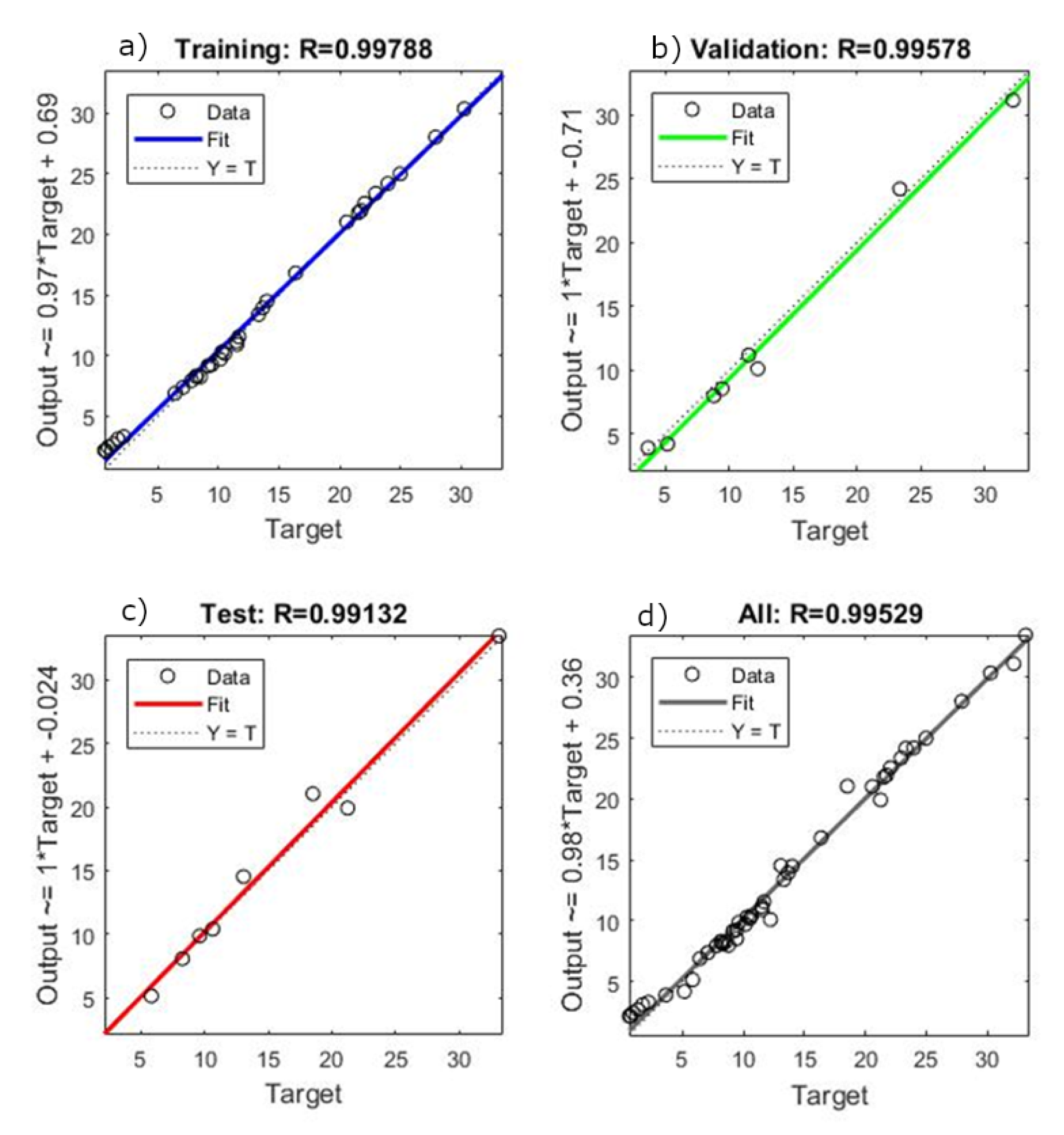
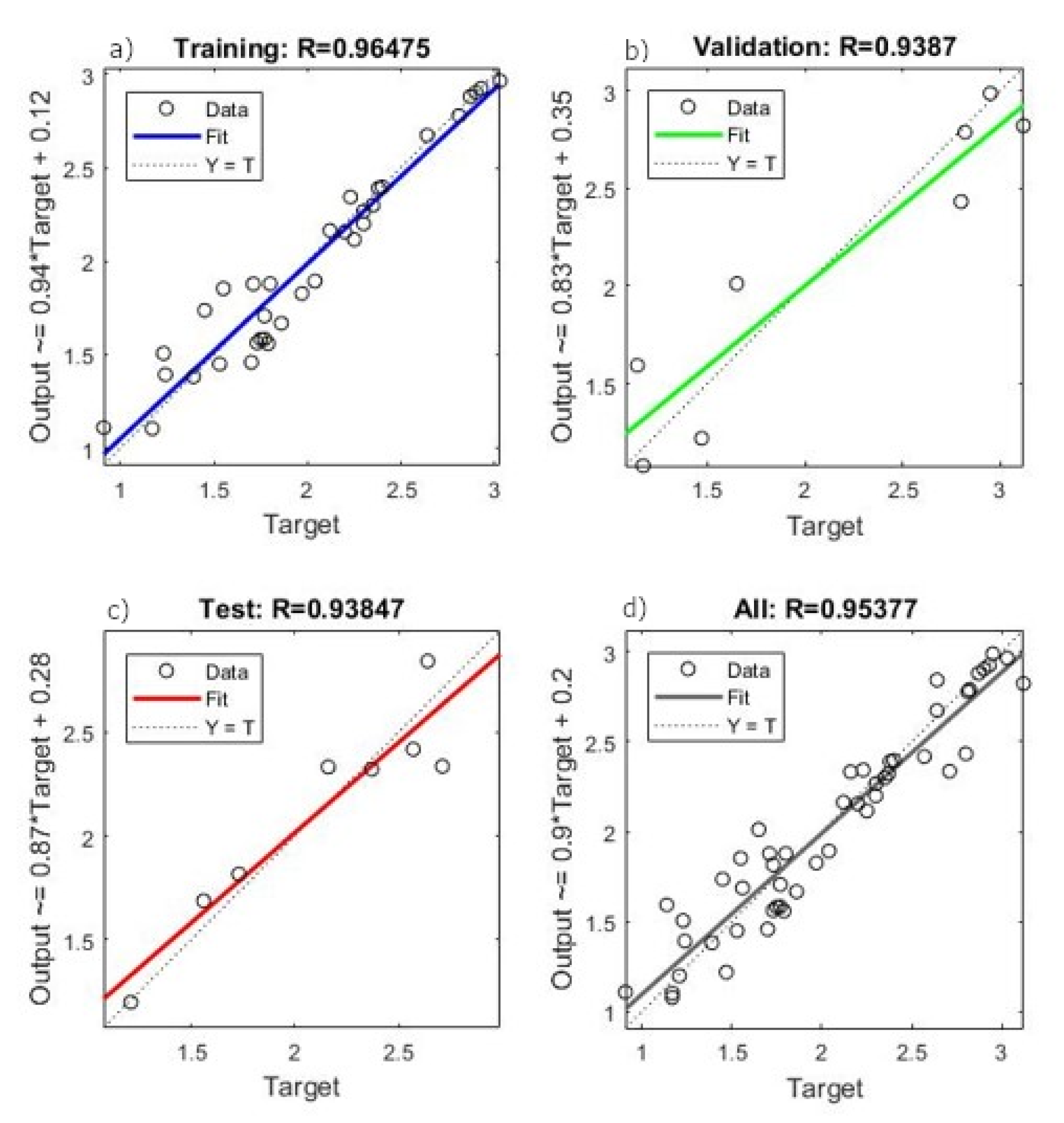
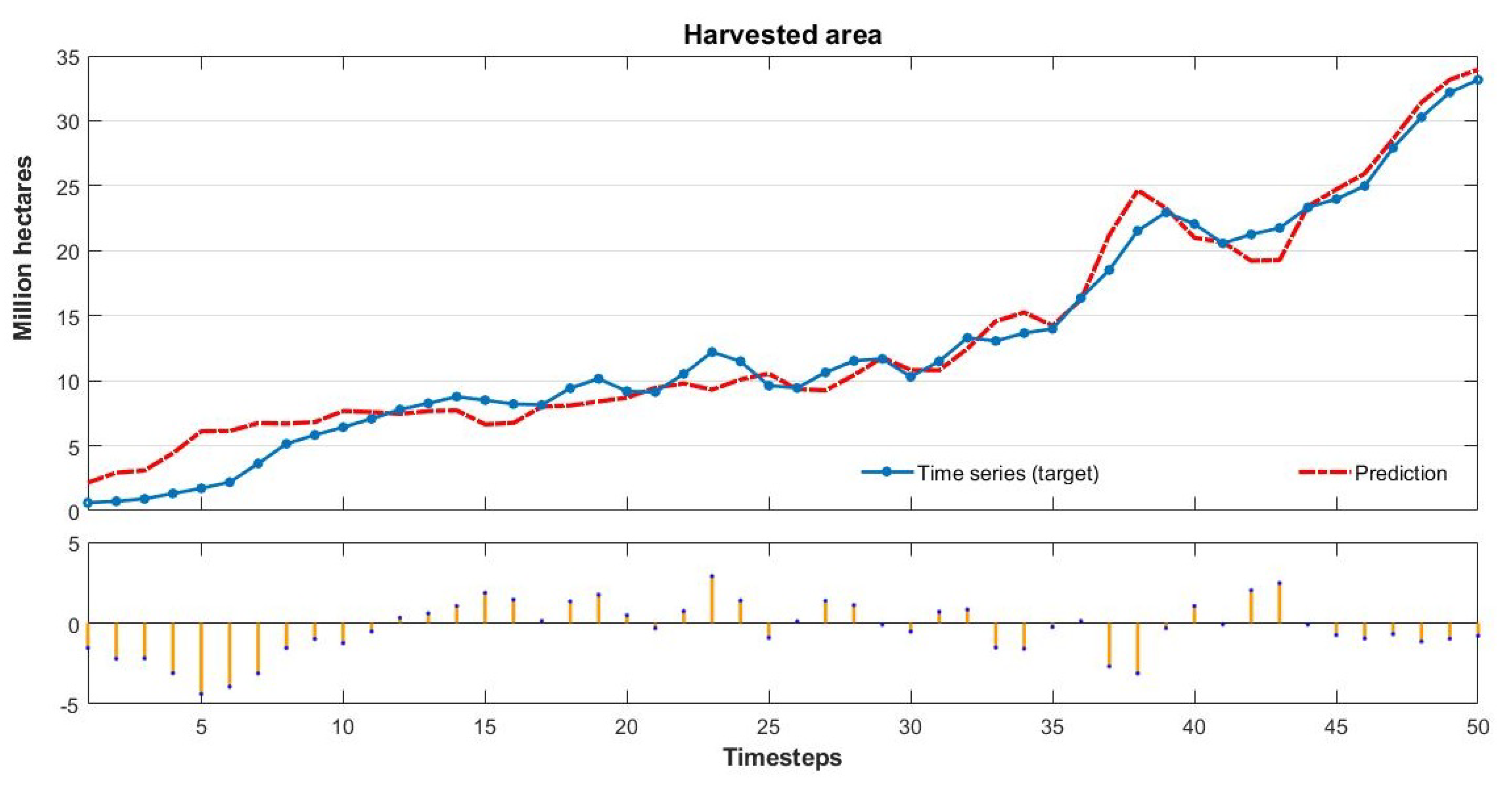
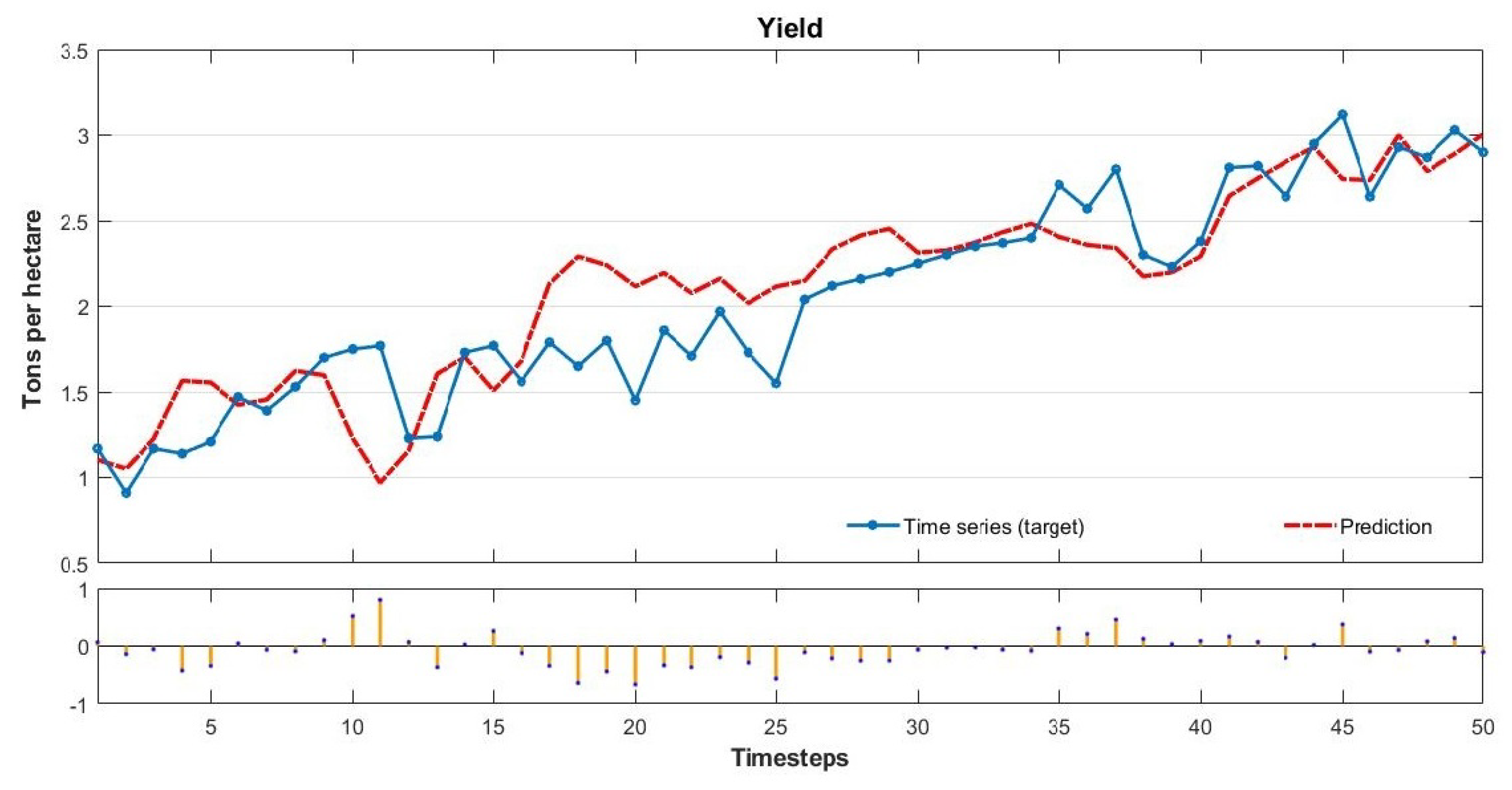
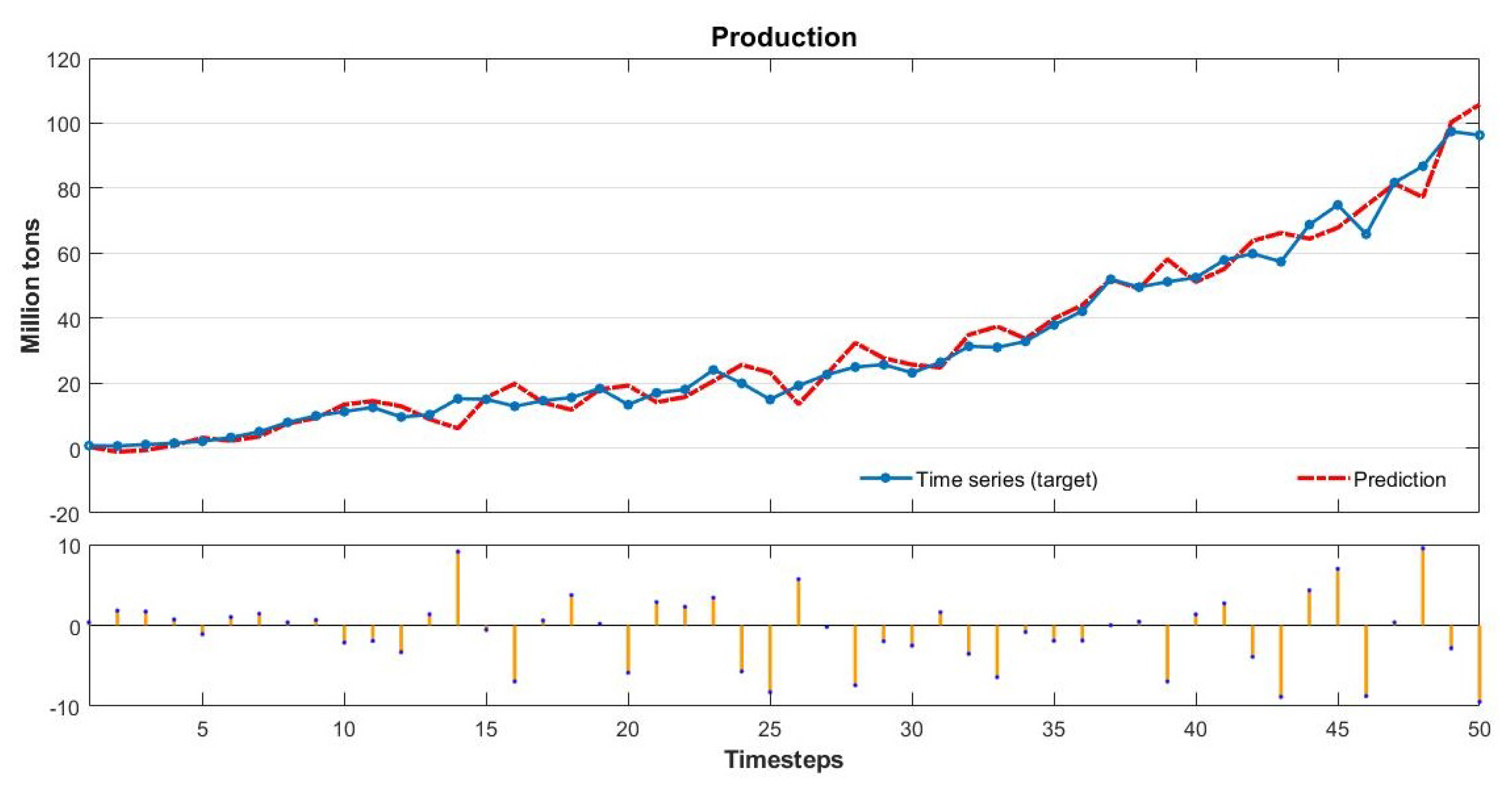
This study compares classical methods of time series prediction with Artificial Neural Networks using Brazilian soybean harvest area, yield and production from 1961–2016. The results indicate that ANN is the best approach to predict soybean harvest area and production while classical linear function remains more effective to predict soybean yield. However, ANN is a reliable model to predict using time series and can help farmers, government, and trading companies anticipate the soybean world offer to organize efficiently logistics resources and public policies.

Our results confirm the important role of neural networks in dealing with agriculture issues as showed in previous studies in the literature [8,10,35,39]. The R value above 0.9 confirms the high performance of the model. Nevertheless, regarding the agriculture concerns about low availability for planting areas, yield, and production [4,5,6], your results demonstrated that, at least in case of the soybean, this is not a concern.

Furthermore, we can conclude that the ANN model can be effective even using a short time series—that, in our case, was 50 years. This fact reveals a robustness of the model. However, despite the advantages of the ANN model, classical methods also can produce very good models. A comparison in other agriculture commodities can be made to confirm or refuse the behavior presented in a soybean case.

Finally, we also suggest for further studies to combine neural networks in hybrid systems using, for example, ANN and Fuzzy Logic, similar to that proposed by [41]. Literature has shown that hybrid systems are more efficient. The goal is to achieve a synergy between hybrid systems to compensate for the disadvantage of one by the advantage of another [55,56,57].

References

1. United Nations. World Population Prospects. In The 2017 Revision. Key Findings and Advance Tables; Technical Report; United Nations Department of Economic and Social Affairs: New York, NY, USA, 2017. [Google Scholar]
2. Alexandratos, N.; Bruinsma, J. World Agriculture towards 2030/2050: The 2012 Revision; Technical Report; Food and Agriculture Organization of the United Nations: Rome, Italy, 2012. [Google Scholar]
3. ONUBR. FAO: Se o Atual Ritmo de Consumo Continuar, em 2050 Mundo Precisará de 60% Mais Alimentos e 40% Mais água. 2015. Available online: https://brasil.un.org/pt-br/68525-fao-se-o-atual-ritmo-de-consumo-continuar-em-2050-mundo-precisara-de-60-mais-alimentos-e-40 (accessed on 19 November 2019).
4. Fukase, E.; Martin, W. Economic growth, convergence, and world food demand and supply. World Dev. 2020, 132, 104954. [Google Scholar] [CrossRef]
5. Fuglie, K.O. Is agricultural productivity slowing? Glob. Food Secur. 2018, 17, 73–83. [Google Scholar] [CrossRef]
6. Rask, K.J.; Rask, N. Economic development and food production–Consumption balance: A growing global challenge. Food Policy 2011, 36, 186–196. [Google Scholar] [CrossRef]
7. Fraanje, W.; Garnett, T. Soy: Food, Feed, and Land Use Change (Foodsource: Building Blocks); Technical Report; Food Climate Research Network, University of Oxford: Oxford, UK, 2020. [Google Scholar]
8. Khan, T.; Qiu, J.; Ali Qureshi, M.A.; Iqbal, M.S.; Mehmood, R.; Hussain, W. Agricultural Fruit Prediction Using Deep Neural Networks. Procedia Comput. Sci. 2020, 174, 72–78. [Google Scholar] [CrossRef]
9. García-Martínez, H.; Flores-Magdaleno, H.; Ascencio-Hernández, R.; Khalil-Gardezi, A.; Tijerina-Chávez, L.; Mancilla-Villa, O.R.; Vázquez-Peña, M.A. Corn Grain Yield Estimation from Vegetation Indices, Canopy Cover, Plant Density, and a Neural Network Using Multispectral and RGB Images Acquired with Unmanned Aerial Vehicles. Agriculture 2020, 10, 277. [Google Scholar] [CrossRef]
10. Maimaitijiang, M.; Sagan, V.; Sidike, P.; Hartling, S.; Esposito, F.; Fritschi, F.B. Soybean yield prediction from UAV using multimodal data fusion and deep learning. Remote Sens. Environ. 2020, 237, 111599. [Google Scholar] [CrossRef]
11. The World Bank. Future Looks Bright for Food Production in Latin America and Caribbean. 2013. Available online: http://www.worldbank.org/en/news/feature/2013/10/16/food-production-trade-latin-america-caribbean-future (accessed on 11 December 2019).
12. Dani, S. Food Supply Chain Management and Logistics: From Farm to Fork, 1st ed.; Kogan Page: London, UK; Philadelphia, PA, USA, 2015. [Google Scholar]
13. EMBRAPA. Embrapa em Números; Technical Report; Empresa Brazileira de Pesquisa Agropecuária-EMBRAPA. Ministério da Agricultura, Pecuária e Abastecimento: Brasília, Brazil, 2017. [Google Scholar]
14. Defante, L.R.; Vilpoux, O.F.; Sauer, L. Rapid expansion of sugarcane crop for biofuels and influence on food production in the first producing region of Brazil. Food Policy 2018, 79, 121–131. [Google Scholar] [CrossRef]
15. USDA. World Agricultural Production: Circular Series November 2019; Technical Report 11-19; USDA: Washington, DC, USA, 2019.
16. Horvat, R.; Watanabe, M.; Yamaguchi, C.K. Fertilizer consumption in the region Matopiba and their reflections on Brazilian soybean production. Int. J. Agric. For. 2015, 5, 52–59. [Google Scholar]
17. Sauer, S.; Pereira Leite, S. Agrarian structure, foreign investment in land, and land prices in Brazil. J. Peasant Stud. 2012, 39, 873–898. [Google Scholar] [CrossRef]
18. Kumagai, E.; Sameshima, R. Genotypic differences in soybean yield responses to increasing temperature in a cool climate are related to maturity group. Agric. For. Meteorol. 2014, 198–199, 265–272. [Google Scholar] [CrossRef]
19. Castanheira, É.G.; Freire, F. Greenhouse gas assessment of soybean production: Implications of land use change and different cultivation systems. J. Clean. Prod. 2013, 54, 49–60. [Google Scholar] [CrossRef]
20. Gil, J.; Garrett, R.; Berger, T. Determinants of crop-livestock integration in Brazil: Evidence from the household and regional levels. Land Use Policy 2016, 59, 557–568. [Google Scholar] [CrossRef] [Green Version]
21. EMBRAPA. Soja em Números. Available online: embrapa.br/web/portal/soja/cultivos/soja1/dados-economicos (accessed on 10 August 2020).
22. United States Department of Agriculture-Economic Research Service. Overview. Available online: https://www.ers.usda.gov/data-products/oil-crops-yearbook/oil-crops-yearbook/#So%20and%20Soybean%20Products (accessed on 10 August 2020).
23. Kaul, M.; Hill, R.L.; Walthall, C. Artificial neural networks for corn and soybean yield prediction. Agric. Syst. 2005, 85, 1–18. [Google Scholar] [CrossRef]
24. Ma, B.L.; Dwyer, L.M.; Costa, C.; Cober, E.R.; Morrison, M.J. Early Prediction of Soybean Yield from Canopy Reflectance Measurements. Agron. J. 2001, 93, 1227–1234. [Google Scholar] [CrossRef] [Green Version]
25. Demuth, H.; Beale, M.; Hagan, M. Neural Network Toolbox User’s Guide; The MathWorks, Inc.: Natick, MA, USA, 2017. [Google Scholar]
26. Russell, S.; Norvig, P. Artificial Intelligence: A Modern Approach, 3rd ed.; Pearson Education India: Bengaluru, India, 2015. [Google Scholar]
27. Aizenberg, I.; Sheremetov, L.; Villa-Vargas, L.; Martinez-Muñoz, J. Multilayer Neural Network with Multi-Valued Neurons in Time Series Forecasting of Oil Production. Neurocomputing 2016, 175, 980–989. [Google Scholar] [CrossRef]
28. Gomes, L.F.A.M.; Machado, M.A.S.; Caldeira, A.M.; Santos, D.J.; Nascimento, W.J.D.d. Time Series Forecasting with Neural Networks and Choquet Integral. Procedia Comput. Sci. 2016, 91, 1119–1129. [Google Scholar] [CrossRef] [Green Version]
29. Wang, J.; Tsapakis, I.; Zhong, C. A space–Time delay neural network model for travel time prediction. Eng. Appl. Artif. Intell. 2016, 52, 145–160. [Google Scholar] [CrossRef]
30. Garg, B.; Kirar, N.; Menon, S.; Sah, T. A performance comparison of different back propagation neural networks methods for forecasting wheat production. CSI Trans. ICT 2016, 4, 305–311. [Google Scholar] [CrossRef]
31. Silva, I.N.D. Redes Neurais Artificiais Para Engenharia e Ciencias Aplicadas: Fundamentos Teoricos e Aspectos Praticos; ARTLIBER: São Paulo, Brazil, 2016. [Google Scholar]
32. Golnaraghi, S.; Zangenehmadar, Z.; Moselhi, O.; Alkass, S. Application of Artificial Neural Network(s) in Predicting Formwork Labour Productivity. Adv. Civ. Eng. 2019, 2019, 1–11. [Google Scholar] [CrossRef] [Green Version]
33. Mohamed, Z.E. Using the artificial neural networks for prediction and validating solar radiation. J. Egypt. Math. Soc. 2019, 27, 47. [Google Scholar] [CrossRef] [Green Version]
34. Almomani, F. Prediction of biogas production from chemically treated co-digested agricultural waste using artificial neural network. Fuel 2020, 280, 118573. [Google Scholar] [CrossRef]
35. Chatterjee, S.; Dey, N.; Sen, S. Soil moisture quantity prediction using optimized neural supported model for sustainable agricultural applications. Sustain. Comput. Inform. Syst. 2018, 100279. [Google Scholar] [CrossRef]
36. Wang, F.; Xiao, H. Prediction on Development Status of Recycle Agriculture in West China Based on Artificial Neural Network Model. In Information Computing and Applications; Zhu, R., Zhang, Y., Liu, B., Liu, C., Eds.; Communications in Computer and Information Science; Springer: Berlin/Heidelberg, Germany, 2010; Volume 105, pp. 423–429. [Google Scholar] [CrossRef]
37. Liu, G.; Yang, X.; Li, M. An Artificial Neural Network Model for Crop Yield Responding to Soil Parameters. In Advances in Neural Networks—ISNN 2005; Hutchison, D., Kanade, T., Kittler, J., Kleinberg, J.M., Mattern, F., Mitchell, J.C., Naor, M., Nierstrasz, O., Pandu Rangan, C., Steffen, B., et al., Eds.; Lecture Notes in Computer Science; Springer: Berlin/Heidelberg, Germany, 2005; Volume 3498, pp. 1017–1021. [Google Scholar] [CrossRef]
38. Fegade, T.K.; Pawar, B.V. Crop Prediction Using Artificial Neural Network and Support Vector Machine. In Data Management, Analytics and Innovation; Sharma, N., Chakrabarti, A., Balas, V.E., Eds.; Advances in Intelligent Systems and Computing; Springer: Singapore, 2020; Volume 1016, pp. 311–324. [Google Scholar] [CrossRef]
39. Zhang, D.; Zang, G.; Li, J.; Ma, K.; Liu, H. Prediction of soybean price in China using QR-RBF neural network model. Comput. Electron. Agric. 2018, 154, 10–17. [Google Scholar] [CrossRef]
40. Abraham, E.R.; dos Reis, J.G.M.; Colossetti, A.P.; de Souza, A.E.; Toloi, R.C. Neural Network System to Forecast the Soybean Exportation on Brazilian Port of Santos. In Advances in Production Management Systems. The Path to Intelligent, Collaborative and Sustainable Manufacturing; Lödding, H., Riedel, R., Thoben, K.D., von Cieminski, G., Kiritsis, D., Eds.; Springer: Cham, Switzerland, 2017; pp. 83–90. [Google Scholar]
41. Abraham, E.R.; dos Reis, J.G.M.; de Souza, A.E.; Colossetti, A.P. Neuro-Fuzzy System for the Evaluation of Soya Production and Demand in Brazilian Ports. In Advances in Production Management Systems. Production Management for the Factory of the Future; Ameri, F., Stecke, K.E., von Cieminski, G., Kiritsis, D., Eds.; IFIP Advances in Information and Communication Technology; Springer: Cham, Switzerland, 2019; Volume 566, pp. 87–94. [Google Scholar] [CrossRef]
42. Escolano, N.R.; Espin, J.J.L. Econometría: Series Temporales y Modelos de Ecuaciones Simultáneas; Limencop: Alicante, Spain, 2012. [Google Scholar]
43. Pecar, B.; Davis, G. Time Series Based Predictive Analytics Modelling: Using MS Excel, 3rd ed.; Amazon Kindle: Seattle, WA, USA, 2018. [Google Scholar]
44. FAO. FAOSTAT. Available online: http://www.fao.org/faostat/en/#data/QC (accessed on 15 December 2019).
45. Shao, Y.E.; Lin, S.C. Using a Time Delay Neural Network Approach to Diagnose the Out-of-Control Signals for a Multivariate Normal Process with Variance Shifts. Mathematics 2019, 7, 959. [Google Scholar] [CrossRef] [Green Version]
46. Di Nunno, F.; Granata, F. Groundwater level prediction in Apulia region (Southern Italy) using NARX neural network. Environ. Res. 2020, 190, 110062. [Google Scholar] [CrossRef] [PubMed]
47. Zhang, J.; Zhang, X.; Niu, J.; Hu, B.X.; Soltanian, M.R.; Qiu, H.; Yang, L. Prediction of groundwater level in seashore reclaimed land using wavelet and artificial neural network-based hybrid model. J. Hydrol. 2019, 577, 123948. [Google Scholar] [CrossRef]
48. Guzman, S.M.; Paz, J.O.; Tagert, M.L.M. The Use of NARX Neural Networks to Forecast Daily Groundwater Levels. Water Resour. Manag. 2017, 31, 1591–1603. [Google Scholar] [CrossRef]
49. Javed, S.; Zakirulla, M.; Baig, R.U.; Asif, S.M.; Meer, A.B. Development of artificial neural network model for prediction of post-streptococcus mutans in dental caries. Comput. Methods Programs Biomed. 2020, 186, 105198. [Google Scholar] [CrossRef]
50. Pereira, L.S. Water, Agriculture and Food: Challenges and Issues. Water Resour Manag. 2017, 31, 2985–2999. [Google Scholar] [CrossRef]
51. Mendes dos Reis, J.G.; Sanches Amorim, P.; Sarsfield Pereira Cabral, J.A.; Toloi, R.C. The Impact of Logistics Performance on Argentina, Brazil, and the US Soybean Exports from 2012 to 2018: A Gravity Model Approach. Agriculture 2020, 10, 338. [Google Scholar] [CrossRef]
52. Schnepf, R.D.; Dohlman, E.; Bolling, C. Agriculture in Brazil and Argentina: Developments and Prospects for Major Field Crops; Technical Report; International Agriculture and Trade Outlook No. (WRS-013); United States Department of Agriculture Economic Research Service: Washington DC, USA, 2001. [Google Scholar]
53. Nedic, V.; Despotovic, D.; Cvetanovic, S.; Despotovic, M.; Babic, S. Comparison of classical statistical methods and artificial neural network in traffic noise prediction. Environ. Impact Assess. Rev. 2014, 49, 24–30. [Google Scholar] [CrossRef]
54. Ko, M.; Tiwari, A.; Mehnen, J. A review of soft computing applications in supply chain management. Appl. Soft Comput. 2010, 10, 661–674. [Google Scholar] [CrossRef] [Green Version]
55. Rajasekaran, S.; Pai, G.A.V. Neural Networks, Fuzzy Logic and Genetic Algorithm: Synthesis and Applications; PHI Learning Pvt. Ltd.: Delhi, India, 2012. [Google Scholar]
56. Roy, S.; Chakraborty, U. Soft Computing: Neuro-Fuzzy and Genetic Algorithms, 1st ed.; Pearson: London, UK, 2013. [Google Scholar]
57. Barrios Rolanía, D.; Delgado Martínez, G.; Manrique, D. Multilayered neural architectures evolution for computing sequences of orthogonal polynomials. Ann. Math. Artif. Intell. 2018, 84, 161–184. [Google Scholar] [CrossRef]
Figure 1. Artificial neuron (left) and ANN multilayer (right).
Agriculture 10 00475 g001
Figure 2. Neural network created in Matlab 2017b.
Agriculture 10 00475 g002
Figure 3. Flowchart of the ANN model.
Agriculture 10 00475 g003
Figure 4. Original time series for harvested area.
Agriculture 10 00475 g004
Figure 5. Original time series for yield.
Agriculture 10 00475 g005
Figure 6. Original time series for production.
Agriculture 10 00475 g006
Figure 7. Regression and correlation of the harvested area using Matlab R2017b.
Agriculture 10 00475 g007
Figure 8. Regression and correlation for yield using Matlab R2017b
Agriculture 10 00475 g008
Figure 9. Regression and correlation for production using Matlab R2017b.
Agriculture 10 00475 g009
Figure 10. Multistep prediction of harvested area using Matlab R2017b.
Agriculture 10 00475 g010
Figure 11. Multistep prediction of yield using Matlab R2017b.
Agriculture 10 00475 g011
Figure 12. Multistep prediction of production using Matlab R2017b.
Agriculture 10 00475 g012