Research Status and Prospects on Plant Canopy Structure Measurement Using Visual Sensors Based on Three-Dimensional Reconstruction

Abstract

Three-dimensional (3D) plant canopy structure analysis is an important part of plant phenotype studies. To promote the development of plant canopy structure measurement based on 3D reconstruction, we reviewed the latest research progress achieved using visual sensors to measure the 3D plant canopy structure from four aspects, including the principles of 3D plant measurement technologies, the corresponding instruments and specifications of different visual sensors, the methods of plant canopy structure extraction based on 3D reconstruction, and the conclusion and promise of plant canopy measurement technology. In the current research phase on 3D structural plant canopy measurement techniques, the leading algorithms of every step for plant canopy structure measurement based on 3D reconstruction are introduced. Finally, future prospects for a standard phenotypical analytical method, rapid reconstruction, and precision optimization are described.

1. Introduction

With the rapid development of plant phenotypical technology, its identification has become a key process used to improve plant yield, and analyzing plant phenotypes with intelligent equipment is one of the main methods to achieve smart agriculture [1]. Digital and visual research of three-dimensional (3D) plant canopy structures is an important part of plant phenotypical studies. With the improvement in computer processing capabilities and reductions in the size of 3D data measurement devices, 3D plant canopy structure measurement and reconstruction studies have begun to increase exponentially [2].

This paper introduces five common visual techniques for 3D plant canopy data measurement, their corresponding instrument models and parameters, and their advantages and disadvantages. These technologies are binocular stereo vision, multi-view vision, time of flight (ToF), light detection and ranging (LiDAR), and structured light. Following this, the general process of 3D reconstruction and structure index extraction of plant canopies are summarized. The accuracy and correlation of the structure index of the reconstructed plant canopy with different visual devices are evaluated, and the common algorithms of plant 3D point cloud processing are reviewed. Then, the technical defects, including the lack of matching between reconstructed 3D plant structure data and physiological data, the low reconstruction accuracy, and the high device costs, are outlined. Finally, the development trends in 3D plant canopy reconstruction technology and structure measurement are described.

2. 3D Plant Canopy Data Measurement Technology

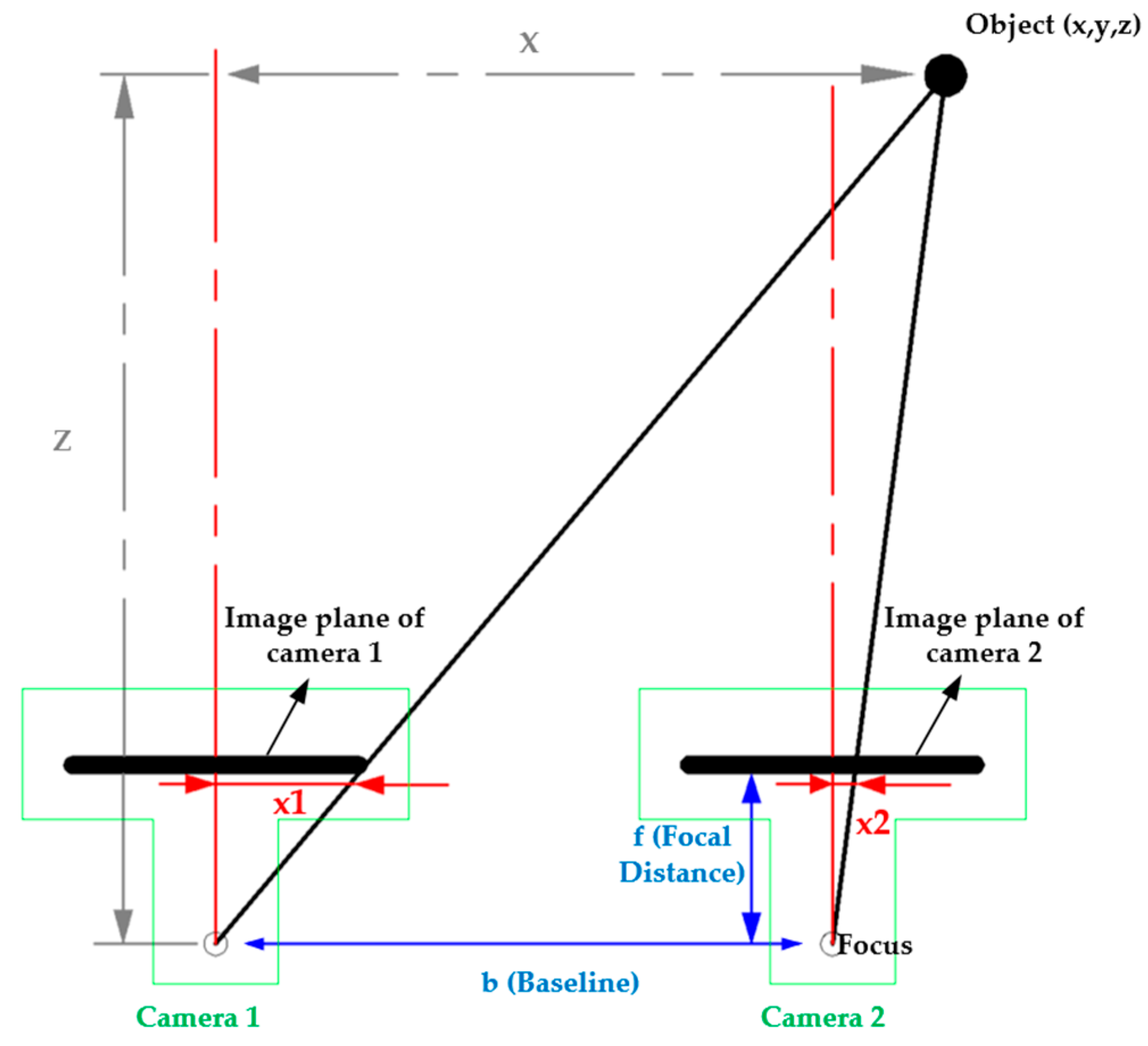
2.1. Binocular Stereo Vision Technology and Equipment

Binocular vision uses two cameras to image the same object at different positions, which will produce a difference in the coordinates of similar features within two stereo images, the difference calls binocular disparity, and the distance (object to camera) can be calculated according to binocular disparity. Disparity distance measurement is applied to calculate depth information [2]. The principle of the method is shown in Figure 1.

The main process of binocular vision reconstruction includes image collection, camera calibration, feature extraction, stereo matching, and 3D reconstruction. Camera calibration is a key step for obtaining stereo vision data with binocular cameras, and its main purpose is to estimate the parameters of a lens and image sensor of a camera, and use these parameters to measure the size of an object in world units or determine the relative location between camera and object. The main camera calibration methods include the Tsai method [3], Faugeras–Toscani method [4], Martins’ two-plane method [5], Pollastri method [6], Caprile–Torre method [7], and Zhang Zhengyou’s method [8]. These methods are based on traditional calibration methods that obtain the camera parameters by using a highly accurate calibration piece to establish the correspondence between the space points and the image points. In addition, there are self-calibration technologies and calibration techniques based on active vision [9]. Andersen et al. [10] used the camera calibration method of Zhang Zhengyou to calibrate the internal parameters of the binocular camera, and then obtained the depth data of wheat using the stereo matching method with simulated annealing.

Stereo matching or disparity estimation is the process of finding the pixels in the multi-view that correspond to the same 3D point in the scene. The disparity map refers to the apparent pixel difference or motion between a pair of stereo images. The calculation of disparity maps in stereo matching is both challenging and the most important part of binocular stereo vision technology. Various algorithms can be used to calculate pixel disparity, which can be divided into global, local, and iterative methods according to different optimization theories; they can also be divided into region matching, feature matching, and phase matching by what elements are represented by the images. Malekabadi [11] used an algorithm based on local methods (ABLM) and an algorithm based on global methods (ABGM) to obtain the disparity image, which can provide plant shape data. Two stereo matchings, 3D minimum spanning tree (3DMST) [12] and semi-global block matching (SGBM), are state-of-the-art and widely used. Bao [13] designed an analysis system to measure plant height in field using a high-throughput field combined with the 3DMST stereo matching technique. Baweja [14] coupled deep convolutional neural networks and SGBM stereo matching to count stalks and measure stalk width. Dandrifosse [15] used SGBM stereo matching to extract wheat structure features with two nadir cameras in field conditions, including height, leaf area, and leaf angles; the result showed that 3D point cloud produced by the stereo camera can be used to measure the plant height and other morphological characteristics, although some errors were noted.

The parameters of typical binocular cameras are shown in

Table 1. Typical binocular stereo camera.

Camera	Bumblebee2-03S2	Zed2	PM802(PERCIPIO)
RGB resolution and frame rate	648 × 488, 48 fps 1024 × 768, 18 fps	4416 × 1242, 15 fps 3480 × 1080, 30 fps 2560 × 720, 60 fps	2560 × 1920, 1 fps 1280 × 960, 1 fps 640 × 480, 1 fps
Depth resolution and frame rate	648 × 488, 48 fps	2560 × 720, 15 fps (Ultra mode)	1280 × 1920, 1 fps 640 × 480, 1 fps
Baseline	120 mm	120 mm	450 mm
Focal length	2.5 mm	2.12 mm	N.A.
Size (mm)	157 × 36 × 47.4	175 × 30 × 33	538.4 × 85.5 × 89.6
Weight (g)	342	135	2000
Measurable range (m)	N.A.	0.5–20	0.85–4.2
Field of view (vertical × horizontal)	66° × 43°	110° × 70°	56° × 46°
Accuracy	N.A.	<1% up to 3 m <5% up to 15 m	0.04–1%
Special or limitations	Extendable	1. Inertial Measurement Unit (IMU) 2. Depending on high-performance equipment	1. Protection: IP54 2. Applying for industry equipment
Price ($)	116	449	11766

N.A. indicates that data were not found; RGB is the abbreviation of red, blue and green.

. Binocular stereo version is simple and inexpensive, and no further auxiliary equipment (such as a specific light source) and no special projection are required [16]. Stereo vision technology also has limitations. It is affected by changes in scene lighting and requires a highly-configured computing system to implement the stereo matching algorithm; The measurement accuracy by binocular stereo depends on the baseline length, as the longer the baseline length compared with distance to a measurement object is, the higher the accuracy is; Stereo vision cannot acquire high-quality data, but it uses the data to have an interpretation in robotics and computer vision [2]; A robust disparity estimation is difficult in areas of homogeneous color or occlusion [16]; and a stereo camera may not reflect the actual boundary of the surface when projecting on a smooth and curved surface, which is called false boundary problem and will affect the correctness of feature matching in active stereo vision. To solve the false boundary problem, one effective approach is to use dynamic and exploratory sensing, another is to move the cameras farther away from the surface [17].

2.2. Multi-View Vision Technology

Multi-view vision technology is an imaging method used to capture pictures of objects from different perspectives with calibrated cameras. The feature points obtained by overlapped images are used to calculate shooting position. Its main applications include structure-from-motion technology (SfM) and multi-view stereo technology (MVS). There are two main multi-view vision technologies: using multiple cameras to obtain 3D data and rotating cameras or objects to obtain 3D data (including deep information). The 3D reconstruction processes for multi-view stereo vision and binocular vision are similar, the biggest difference is that SfM uses redundancy overlapping images to get camera position parameters, and binocular vision uses a traditional calibration method, calibration, matching, and 3D reconstruction. Although the image produced by multi-view vision is more accurate, its calibration and synchronization, including camera location mainly, are more complicated than those of a binocular camera.

SfM and MVS have a sequential order: SfM is used to determine camera poses, intrinsic parameters calibration and start feature matching, then MVS is used to reconstruct the dense 3D scene. Structure-from-motion technology (SfM) is a distance imaging technology that estimates a 3D structure by capturing a series of 2D images at different locations in a scene, whose model includes incremental, global, and hybrid structures, then it applies a highly redundant image feature and matches the 3D positions of features based on the scale-invariant feature transform (SIFT) algorithm (or using SURF, ORB algorithm). After estimating camera pose and extracting the points cloud (using Bundler), MVS technology is used to reconstruct a complete 3D object model from a suite of images taken from known camera locations after calibrating cameras [18], which uses the method of polar geometric constraint that sees whether they are consistent with a common popular geometry to match each pixel (clustering views for multi-view stereo (CMVS), patches-based multi-view-stereo (PMVS2) algorithms and et al.). Some open source software for MVS are shown in

Table 2. Open source software for multi-view stereo technology (MVS).

Project	Colmap	GPUlma + Fusibile	HPMVS	MICMAC	MVE	OpenMVS	PMVS
Language	C++ CUDA	C++ CUDA	C++	C++	C++	C++ CUDA	C++ CUDA

CUDA: Compute Unified Device Architecture.

.

SfM generally produces sparse point clouds and MVS photogrammetry algorithms are used to increase the point density by several orders of magnitude. As a result, the combined workflow is more correctly referred to as ‘SfM-MVS’ [19]. The steps of point cloud formation based on SfM-MVS generally include feature detection, keypoint correspondence, identifying geometrically consistent matches, structure from motion, scale and georeferencing, refinement of parameter values, and multi-view stereo image matching algorithms. Some typical commercial integrated software for implementing SfM-MVS are shown in

Table 3. Commercial software for 3D scene modeling utilizing SfM-MVS.

Name	Function	Company
ContextCapture	Create detailed 3D models quickly with simple photos	Bentley Acute3D
PhotoMesh	Construct full-element, fine, textured three-dimensional mesh models from a set of standard, disordered two-dimensional photographs.	SkyLine
StreetFactory	Enabling rapid and fully automatic process of images from any aerial or street camera for the generation of a 3D textured database and distortion-free imagery	AirBus
PhotoScan	Performing photogrammetric processing of digital images and generates 3D spatial data to be used in geographic information system (GIS) applications	AgiSoft
Pix4DMapper	Transform images in digital maps and 3D models.	Pix4D
RealityCapture	Extracts accurate 3D models from a set of ordinary images and/or laser scans	RealityCapture

.

Scale and georeferencing are special steps for aerial maps. Output of the SfM stage is a sparse unscaled 3D point cloud in arbitrary units along with camera models and poses, so correct scale, orientation, or absolute position information need to be built according to known coordinates. Three methods can be used to enable accurate scale and georeferencing of the imagery. One is using a minimum of three ground control points (GCPs) with XYZ coordinates to scale and georeference the SfM-derived point cloud [20]. Orientation can be measured from an Inertial Measurement Unit (IMU) [21] and it can be performed from known camera positions derived from RTK-GPS measurements [22]. On the other hand, the metric scaling factor was derived through the known value of a geometrical feature in the point cloud for small-scale plant measurement without unmanned aerial systems (UAS), and raw point cloud are multiplied by a scale factor that is the ratio of the feature in millimeters and in the pixel system of the raw point cloud, which will determine an individual scale factor for every point cloud [23].

SfM can be applied to large-scale plant measurement. Unmanned aerial systems are necessary pieces of auxiliary equipment for large-scale experimental field measurement based on SfM-MVS. Images are acquired autonomously based on presetting UAS parameters and camera settings, then point cloud data are generated by some commercial software for 3D scene modeling. Then plant height, density, and etc. was calculated after point cloud processing. For example, Malambo [20] used a DJI ^® Phantom 3 to acquire images and 6 or more portable GCPs were placed uniformly in the field and measured using a Trimble GeoXH GPS system for scale and georeferencing, 100 readings were taken per point and differentially post-processed using Trimble’s Pathfinder Office software to achieve centimeter accuracy (<10 cm), and Pix4Dcapture software based on SfM was used to generate a point cloud, then point cloud was processed to obtain maize height. SfM can also be applied to small-scale plant measurement. Rose [23] used Pix4DMappe based on SfM-MVS to reconstruct single tomato plants, and extracted main stem height and convex hull from the 3D point clouds.

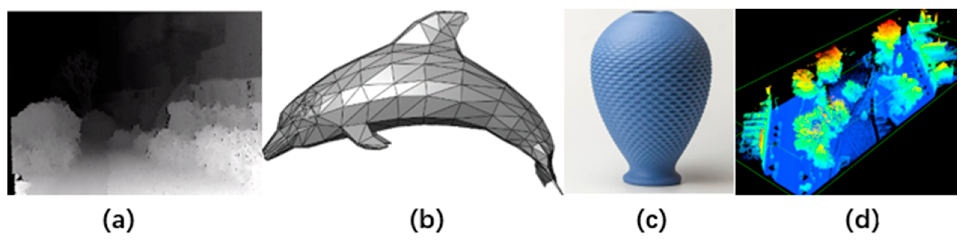
2.3. Time of Flight Technology

Time of Flight (ToF) is a high-precision ranging method. ToF cameras and LiDAR (light detection and ranging) scanning are based on Time of Flight technology. The imaging principles of ToF can be divided into pulsed-wave (PW-iToF) or continuous-wave (CW-iToF) modulation [24]. The ToF imaging principle is shown in Figure 2. CW-iToF emits near-infrared (NIR) light through a light-emitting diode (LED), which reflects back to the sensor. Each pixel on the sensor samples the amount of light reflected by the scene four times in equal intervals per cycle (such as m0, m1, m2, and m3). The phase difference, offset value, and amplitude are sampled by comparing the modulation phase with the transmitted signal phase, and the target depth is calculated based on these three quantities. PW-iToF uses a transmitting module to transmit a laser pulse (Tpulse), while at the same time, a shutter pulse, which has the same time length with Tpulse, is activated by the transfer gate (TX1). When the reflected laser hits the detector, the charges are collected. After the first shutter pulse ends, the second shutter pulse is activated by the transfer gate (TX2). The charge is integrated in the according storage node of two shutters and the target depth is calculated based on accumulation of charge [24].

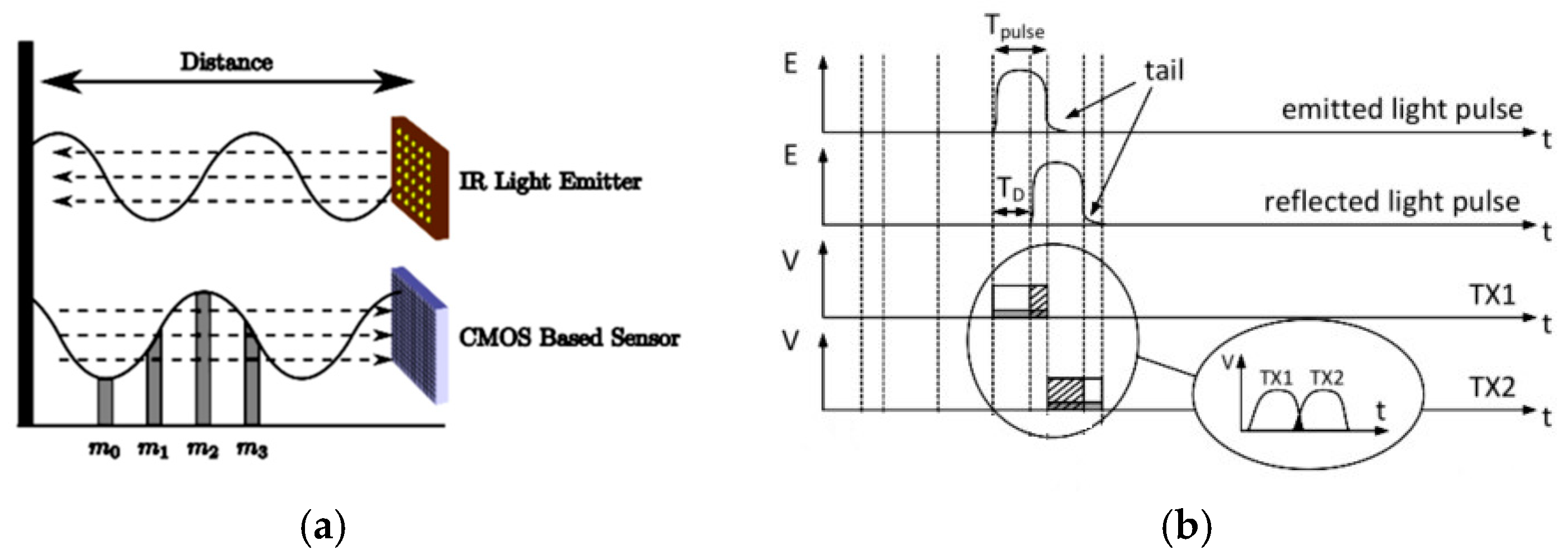
2.3.1. Time of Flight Cameras

Time of Flight cameras are part of a broader class of scannerless LiDAR, in which the entire scene is captured with each laser pulse, as opposed to point-by-point with a laser beam, such as in scanning LIDAR systems [25]. Typical cameras using ToF technology are SR-4000, CamCube, Kinect V2, etc., whose structural parameters are shown in

Table 4. Depth camera comparison based on time of flight (ToF).

Camera	CAMCUBE 3	SR-4000	Kinect V2	IFM Efector 3D (O3D303)
Manufacturer	PMD Technologies GmbH	Mesa Imaging AG	Microsoft	IFM
Principle	Continuous-wave modulation	Continuous-wave modulation	Continuous-wave modulation	Continuous-wave modulation
V (vertical) × H (horizontal) field of view	40° × 40°	N.A.	70° × 60°	60° × 45°
Frame rate and depth resolution	40 fps, 200 × 200	54 fps, 176 × 144	30 fps, 512 × 424	40 fps, 352 × 264
Measurable range (m)	0.03–7.5	0.03–7.5	0.5–5	0.03–8
Focal length (m)	0.013	0.008	0.525	N.A.
Signal wavelength (nm)	870	850	827–850	850
Advantages	Strong resistance to ambient light, high precision	High precision and light weight	Rich development resource bundle	Not affected by light, detection of scenes and object without 3D images of motion blur
Disadvantages	High cost	Not for outdoor light	Low measurement accuracy; not suitable for very close object recognition	High cost

. An important issue for ToF cameras is the wrapping effect, which is the distances to objects that differ 360° in phase and are indistinguishable. Multiple modulated frequencies and lowering the modulation frequency can solve the issue by increasing the unambiguous metric range [26]. Hu et al. [27] proposed an automatic system for leaflet non-destructive growth measurement based on a Kinect V2, which uses a turntable to obtain a multi-view 3D point cloud of the plant under test. Yang Si et al. [28] used a Kinect V2 to obtain the 3D point cloud depth data of vegetables in seedling trays. Vázquez–Arellano [29] estimated the stem position of maize plant clouds, calculated the height of individual plants, and generated a plant height profile of the rows using a Kinect V2 camera in a greenhouse. Bao [30] used Kinect V2 to obtain 3D point cloud data under field conditions, and a point cloud processing pipeline was developed to estimate plant height, leaf angle, plant orientation, and stem diameter across multiple growth stages. A branch 3D skeleton extraction method based on an SR4000 was proposed by Liu [31] to reconstruct a 3D skeleton model of the branches of apple trees, and an experiment was carried out in Fruit Tree Experimental Park; Skeletonization is the process of calculating a thin version of a shape to simplify and emphasize the geometrical and topological properties of that shape, such as length, direction, or branching, which are useful for the estimation of phenotypic traits. Hu [32] used the SR4000 camera to acquire a plant’s 3D spatial data and construct a 3D model of poplar seedling leaves, then calculated leaf width, leaf length, leaf area, and leaf angle based on the 3D models.

A key advantage of time-of-flight cameras is that only a single viewpoint is used to compute depth. This allows robustness to occlusions and shadows and preservation of sharp depth edges [33]. The main disadvantages of Time of Flight are low resolution, and not being to able to be operated under strong sunlight, being disturbed by other’s ToF cameras, and short distance measurement.

2.3.2. LiDAR Scanning Equipment Based on ToF

Light detection and ranging (LiDAR) was developed in the early 1970s to monitor the earth [34]. LiDAR can be divided into aerial and terrestrial LiDAR. As aerial LiDAR laser scanning is mainly used for 3D data measurement of glaciers, forests, and land, the effect resolution is low in plant phenotypical analysis, so terrestrial LiDAR scanning is mainly used in 3D plant scanning. Terrestrial LiDAR (T-LiDAR) scanners can be divided into phase-shift T-LiDAR and pulse-wave T-LiDAR. T-LiDAR estimates time by the phase shift between the continuous emission and the receipt of the laser beam, making it ideal for measuring high-precision and relatively close scenarios. Time-of-flight T-LiDAR is based on calculating the time between emitting and receiving laser pulses to estimate the distance, which is suitable for scenarios with large distances. The specification parameters of partial low-cost devices T-LiDAR for measurements of a plant canopy are shown in

Table 5. Low-cost T-LiDAR (Terrestrial LiDAR) scanners specifications.

Performance Parameters	LMS 111 [35]	UTM30LX [36,37]	LMS291-S05 [38]	Velodyne HDL64E-S3 [39]	FARO Focus 3D X 330 HDR [40]
Measurement range (m)	0.5–20	0.1–30	0.2–80	0.02–120	0.6–330
Field of view (vertical × horizontal)	270° (H)	270° (H)	180° (H)	26.9° × 360° (V × H)	300° × 360° (V × H)
Light source	Infrared (905 nm)	Laser Semicon-ductor (905 nm)	Infrared (905 nm)	Infrared (905 nm)	Infrared (1550 nm)
Scanning frequency (Hz)	25	40	75	20	97
Angular resolution (°)	0.5	0.25	0.25	0.35	0.009
Systematic error	±30 mm	N.A.	±35 mm	N.A.	±2 mm
Statistical error	±12 mm	N.A.	±10 mm	N.A.	N.A.
Laser class	Class 1 (IEC 60825-1)	Class 1	Class 1 (EN/IEC 60825-1)	Class 1 (Eye-safe)	Class 1
Weight (kg)	1.1	0.21	4.5	12.7	5.2
LiDAR specifications	2D	2D	2D	3D	3D

N.A. indicates that data were not found.

.

LiDAR can be used for canopy measurement. Garrido [35] used portable LiDAR LMS 111 to reconstruct a maize 3D structure under greenhouse conditions, which can help the aim of developing a georeferenced 3D plant reconstruction. Yuan [38] developed a detection system to measure the tree canopy structure by LiDAR UTM30LX and the height and weight of artificial tree could be obtained by the system. Qiu [39] used LiDAR Velodyne HDL64E-S3 to get depth-band histograms and horizontal point density, using the data to recognize and compute the morphological phenotype parameters (row spacing and plant height) of maize plants in the experimental field. Jin [40] used LiDAR FARO Focus 3D X 330 HDR to get maize point cloud data, and realized stem-leaf segmentation and phenotypic trait extraction in an experiment carried out in the Botany Garden.

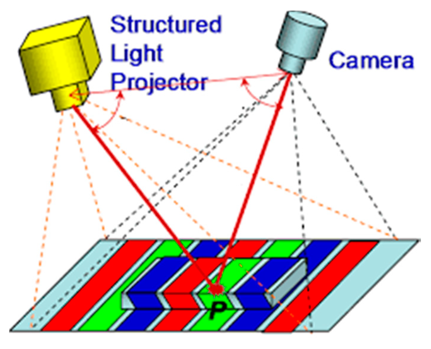
2.4. Structured Light Technology and Equipment

Structured light is an active imaging technology. The projector projects a series of light sequences, or patterns consisting of many stripes at once or of arbitrary fringes onto the object, and the light sequence is deformed on the object. Then, the camera shoots the object in another direction and extracts the deformation of its stripe shape and stripe width to obtain depth data. The method is shown in Figure 3.

A structured light 3D scanner has some advantages. A structured light scanner can produce highly accurate results, resolution is typically high, the images captured can reliably determine the dimensions of the object, and it is often fast. 3D imaging can occur practically as fast as an image can be taken. Structured light scanner imaging systems have a better measurement coverage area than other 3D imaging techniques, as long as the distance is fixed. This is particularly useful for larger parts that need multiple scans, further saving time and creating efficiencies in production [33]. Major drawbacks of the sequential projection techniques include its inability to acquire the 3D object in dynamic motion or in a live subject such as human body parts. Another limitation is that the reflected pattern is sensitive to optical interference from the environment, so it is suitable for indoors. The general process for 3D reconstruction based on structured light is as follows: camera and projector calibration, projector calibration includes intensity calibration to build the relationship between the actual intensity of the projected pattern and image pixel value, geometric calibration to build the relationship between point of 3D space and projector [41], projecting patterns and finding correspondences to estimate parameter matrix between pixel and point of 3D space, obtaining a 3D point cloud based on the parameter matrix of the structured light camera, and to carry out 3D reconstruction.

Chené et al. [42] used Kinect V1 to measure leaf curvature, morphology, and orientation. Azzari et al. [43] used Kinect V1 to obtain the point cloud data of the plant, and then constructed the canopy structure of the plant to obtain the plant diameter and height. Nguyen et al. [44] used a combination of structured light and a multi-camera to extract plant (cabbage, cucumber, tomato) height, leaf area, and total shaded area. Syed et al. [45] used Realsense SR300 to obtain the color and depth data of the plants (pepper, tomato, cucumber, and lettuce), with the key characteristics of the seedlings obtained through a series of algorithms; the processing speed was also fast. Vit [46] compared the following sensors: Kinect II, Orbbec Astra, Intel RealSense SR300, and Intel D435; and experiments showed that the Intel D435 sensor provided the best accuracy for measuring the average diameter of maize stems. Liu [47] proposed a recognition algorithm for citrus fruit based on RealSense. The method effectively used depth-point cloud data got from RealSense F200 in a close-shot range of 160 mm and different geometric features of the citrus fruit and leaves to recognize fruits with an intersection curve cut by the depth-sphere. Milella [48] used the RealSense R200 depth camera to construct an in-field high throughput grapevine phenotyping platform that can estimate canopy volume and detect grape bunches under field condition. And some structured light depth cameras specifications are shown in

Table 6. Depth camera comparison based on structured light.

Performance Parameters	Kinect V1	RealSense SR300	Orbbec Astra	Occipital Structure
Measurable range (m)	0.5–4.5	0.2–2	0.6–8	0.4–3.5
V × H field of view	57° × 43°	71.5° × 55°	60° × 49.5°	58° × 45°
Frame rate and depth resolution	30 fps, 320 × 240	60 fps, 640 × 480	30 fps, 640 × 480	60 fps, 320 × 240
Price ($)	199	150	150	499
Size (mm)	280 × 64 × 38	14 × 20 × 4	165 × 30 × 40	119.2 × 28 × 29

.

2.5. Comparison of Main Measurement Technologies

Table 7. Summarize the advantages and disadvantages of each technology.

Category	Advantages	Disadvantages
Binocular stereo vision technology [49]	(1) Get depth image quickly and plant’s slight movement does not affect the precision (2) Low cost (3) Obtains deep and color data at the same time (4) No further auxiliary equipment	(1) Affected by scene lighting (2) High computer performance and complicated algorithm (3) Complex 3D scene reconstruction (4) Not for homogeneous color (5) False boundary problem
Structure-from- motion technology [50]	(1) Operates easily and low cost (2) Open source and commercial software for 3D reconstruction (3) Suitable for aerial applications, excellent portability	(1) Not suitable for real-time applications
Time-of-flight technology [49,51]	(1) No external light (2) Single viewpoint to compute depth	(1) Poor depth resolution (2) Not work in bright light (3) Short distance measurement
LiDAR scanning technology	(1) Fast image collection (2) Can work at night (3) Can work in severe weather (rain, snow, fog, etc.) for advanced laser scanning (4) Works over long distances (more than 100 m)	(1) Poor edge detection (3D point clouds of edges of plant organs like leaves, for instance, are blurry) (2) Needs warm-up time (3) Need for movement to obtain the depth data of the detected object
Structured light technology	(1) Accuracy and high depth resolution (2) Get depth image quickly (3) Captures large area	(1) Indoor plant imaging (2) Stationary object

summarizes the devices’ technology differences of stereo vision, SfM, Time of Light, LiDAR scanning, and structured light in 6 aspects. The numbers of plus and minus are intensity of advantage.

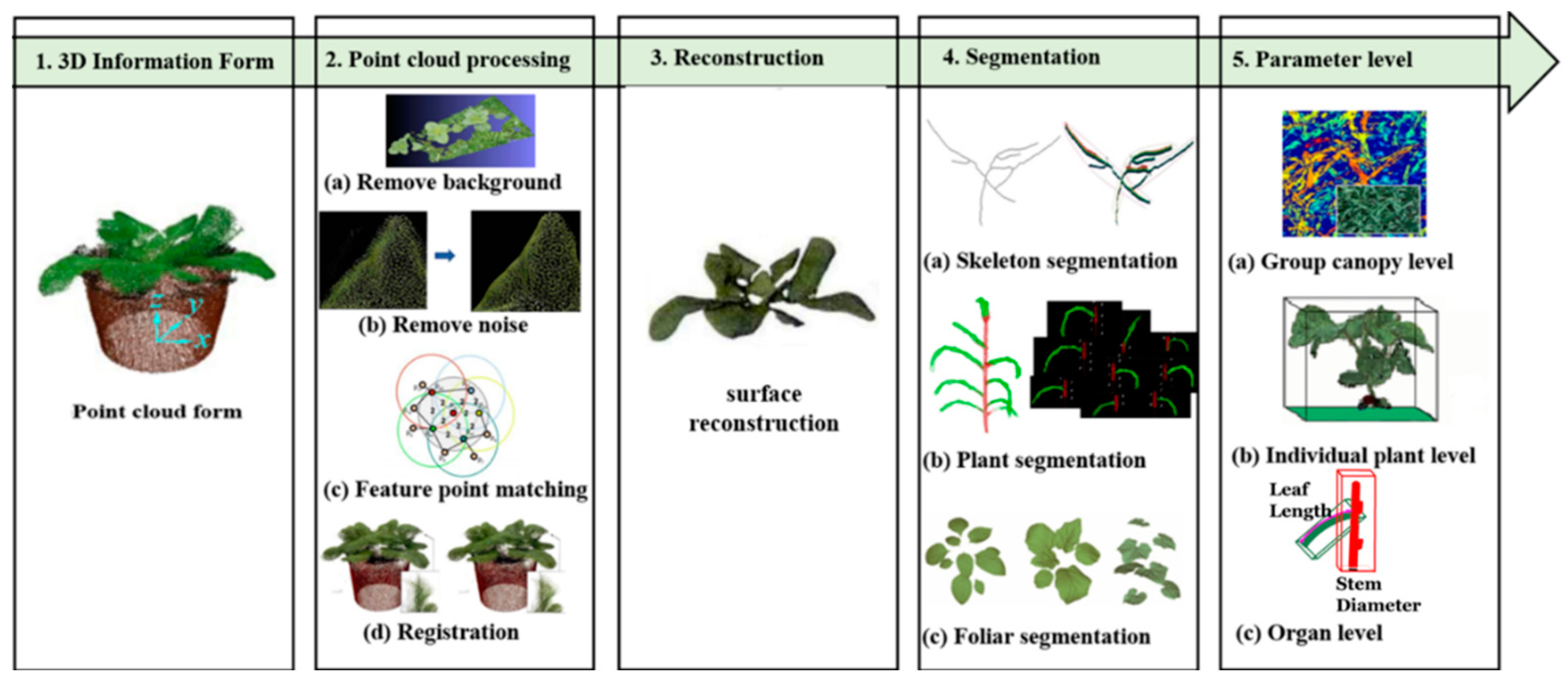
3. Plant Canopy Structure Measurement Based on 3D Reconstruction

Plant canopy structure measurement based on 3D reconstruction main flows include 3D plant data acquisition, point cloud processing, 3D plant reconstruction, plant segmentation, plant canopy structure parameters extraction. The processes are shown in Figure 4.

3.1. 3D Plant Data Acquisition

Plant 3D data are mainly displayed using depth maps [52,53], polygon meshes [54], voxels [55,56,57,58], and 3D point clouds [44]. The presentation of data types is shown in Figure 5. Among them, the depth map is a 2D picture, and each pixel value records the distance from the camera viewpoint to the surface of the obstruction. A polygon mesh, also called an unstructured mesh, is a collection of vertices and polygons representing polyhedron shapes in 3D computer graphics, consisting of a series of convex polygon vertices and convex polygon surfaces [59]. Polygon meshes are intended to represent 3D object models in a way that is easy-to-render. A voxel [60], which is an abbreviation for volume cell and is similar to a pixel of 2D space, is the smallest unit of digital data in the 3D space partition. Voxelization is a standardized representation method that is used in the field of 3D imaging. A point cloud is a data set of points in a certain coordinate system that includes 3D coordinates, color, size value, segmentation results, etc.

3D point cloud data can be obtained by a visual sensor based on binocular stereo vision technology, multi-view vision technology, SfM technology, ToF technology, and so on. The details of the technical principle and camera specifications are shown in Section 2.

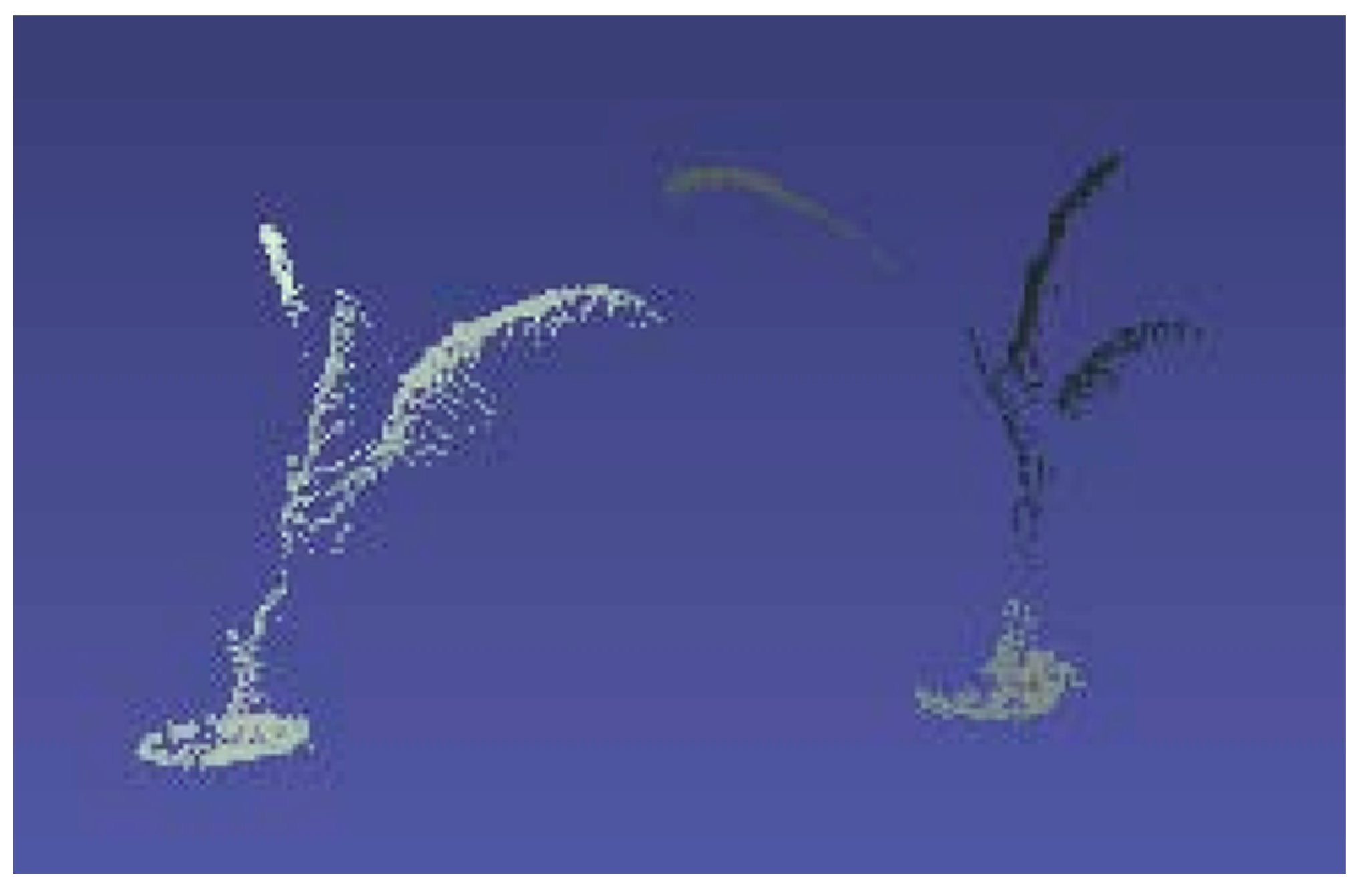
3.2. 3D Plant Canopy Point Clouds Preprocessing

Modeling using point cloud data is fast and has finer details than polygon meshes and voxels, which is valuable for agricultural crop monitoring. However, point clouds cannot be used directly for 3D applications, they need to be processed first because of wrongly assigned points and no-interest points, which are not matching between pixel point and actual corresponding object, or it is background and no target object. 3D point cloud preprocessing in general includes background subtraction, outlier removal, and denoising [61]. At present, there are many open source resources available for point cloud processing.

Table 8. Introduction of open source libraries and software for point cloud processing.

Type	Name	Function	Reference URL
Open source library	Point Cloud Library	Large cross-platform open-source C++ programming library providing a full set of point cloud data processing modules to implement a large number of general point-cloud-related algorithms and efficient data structures	http://pointclouds.org/
	Point Data Abstraction Library	C++ BSD (the Berkeley software distribution) library for translation and manipulation of point cloud data	https://pdal.io/
	Liblas	Libraries for reading and writing plain LiDAR formats	https://liblas.org/
	Entwine	Data organization library for a large number of point clouds, designed to manage hundreds of millions of point and desktop-scale point clouds	https://github.com/connormanning/entwine/
	PotreeConverter	Data organization library that generates data for data used in Potree (a large network-based point cloud renderer) network viewer	https://github.com/potree/PotreeConverter
Open source software	Paraview	Multi-platform data analysis and visualization application	https://www.paraview.org/
	Meshlab	Open source for unstructured 3D triangular mesh processing and editing; portable and scalable system	http://meshlab.sourceforge.net/
	CloudCompare	3D point cloud and grid processing software open source project	http://www.danielgm.net/cc/
	OpenFlipper	Multi-platform application and programming framework designed to process, model, and render geometric data	http://www.openflipper.org/
	PotreeDesktop	Desktop/portable version of the web-based point cloud viewer Potree	https://github.com/potree/PotreeDesktop
	Point Cloud Magic	The first set of free point cloud data processing “point cloud cube” software developed by the Chinese Academy of Sciences for remote sensing of the earth, LiDAR statistical parameters, extraction of vegetation height, biomass, etc., based on statistical regression methods and single tree segmentation	http://lidar.radi.ac.cn/

introduces some functions of open source point cloud processing libraries and open source software.

3.2.1. Background Subtraction

To obtain only the plant canopy, it is necessary to separate the plant point cloud area from the ground, weeds, or other backgrounds after obtaining plant 3D point clouds data. When using active image technology (ToF technology, structured light technology, and so on) without color data to get 3D point clouds, detection of geometric shapes can be applied to remove the background. When using passive image technology (binocular stereo vision technology, multi-view vision technology, SfM technology, and so on), color thresholding or clustering with different color data can be applied to remove background.

Bao [13] uses the Random Sample Consensus (RANSAC) algorithm to fit a plane, and subtracts the background whether un-requiring the distance threshold value between data point and defined plane. Klodt [62] used dense stereo reconstruction to analyze grapevine phenotyping, and backgrounds were segmented with respect to the color and depth information. However, the low-level geometric shapes features cannot handle all types of meshes. Deep Convolutional Neural Networks (CNNs) can solve the problem and provide a highly accurate way to label the background, using many geometric features to train a label model [63].

Background subtraction has an important application in robotic weeding. Plant recognition for automated weeding based on 3D sensors included preprocessing, ground detection, plant extraction refinement, and plant detection and localization. Gai [64] used Kinect V2 to obtain broccoli point clouds and RANSAC was used to remove ground Afterwards, 2D color information was utilized to compensate rough ground error and clustering was applied to remove weeding point cloud, and the result after ground removal with RANSAC is shown in Figure 6. Andújar [65] used Kinect V2 for volumetric reconstruction of corn, and canonical discriminant analysis (CDA) was used to predict weed classification of the system using weed height.

3.2.2. Outlier Removal and Plant Point Clouds Noise Reduction

An outlier is a data point that differs significantly from other observations. Noisy data are with a large amount of additional meaningless information data, which arise out of various physical measurement processes and limitations of the acquisition technology [66], including being corrupted or distorted, or having a low signal-to-noise ratio data. Also, matching ambiguities and image imperfection produced by lens distortion or sensor noise will lead to outliers and noise of point cloud data. Outlier detection approaches are classified into distribution-based [67], depth-based [68], clustering [69], distance-based [70], and density-based approaches [71]. The moving least-squares (MLS) generally deals with noise, which iteratively projects points on weighted least squares fits of their neighborhoods, thus causing the newly sampled points to lie closer to an underlying surface [72].

Wu et al. [73] used a statistical outlier removal filtering algorithm to denoise the point cloud, which calculates the mean distance to the K neighboring points by K-neighbor searching method for each point, and removing oversize value. Yuan et al. [38] used statistical outliers to remove outlier point clouds around peanut point clouds. Wolff [74] designed a new algorithm to remove noisy points and outliers from each per-view point cloud by checking if points are consistent with the surface implied by the other input views. Xia [75] combined the two characteristic parameters of the average distance of neighboring points and the number of points in the neighborhood to remove outlier noise, and used a bilateral filtering algorithm to remove small noise in the point cloud of tomato plants. After performing point-wise Gaussian noise reduction, Zhou et al. [76] used the grid optimization method to optimize the point cloud data, and used the average distance method to remove redundant boundary points, thus obtaining a more realistic blade structure. Hu et al. [27] first used the multi-view interference elimination (MIE) algorithm to reduce layers and then used moving least squares (MLS) algorithm to reduce the remaining local noise.

3.3. 3D Plant Canopy Reconstruction

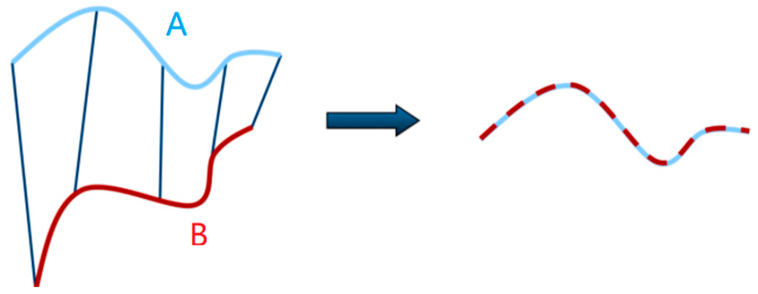
3.3.1. Plant Point Clouds Registration

To measure the complete data model of a plant, the points obtained from various perspectives are combined into a unified coordinate system to form a complete point cloud, so the point clouds needs to be registered. The purpose of registration is to transform the coordinates of the source point cloud (initialized the point cloud) and target point cloud (point cloud formed by the motion of targeted object), and obtain a rotation translation matrix (RTMatrix, RTRT) that represents the position transformation relationship between source point cloud and target point cloud. Point cloud registration can be divided into rough registration and precise registration. Rough registration uses rotation axis center coordinate and rotation matrix to make the rigid transformation of point clouds. Precise registration aligns two sets of 3D measurements from geometric optimization. Iterative closing point (ICP) algorithm [77], Gaussian mixture models (GMM) algorithm [78] and thin plate spline robust point matching (TPS-RPM) algorithm [79] are generally used to make precise registration. ICP is the most classic and easy, which iteratively calculates the distance between the corresponding source point cloud and the target point cloud, constructing a rotation translation matrix to transform the source point cloud, and calculating the mean squared error after the transformation to determine if met defined threshold. Jia [80] performed the rough registration of plant point clouds from six perspectives based on the sample consistent initial alignment (SAC_IA). Precise registration uses a known initial transformation matrix, and it obtains a more accurate solution through ICP algorithm. The principle of ICP algorithm is shown in Figure 7.

3.3.2. Plant Point Clouds Surface Reconstruction

According to the different principles of reconstruction surfaces, 3D point clouds surface reconstruction can be divided into surface reconstruction based on Delaunay triangulation [81], region-based growth surface reconstruction, and implicit surface reconstruction [82]. Among them, the Delaunay triangulation and its improved method [83,84,85] can satisfy the consistency requirements of the point cloud data topology, but the accuracy of surface reconstruction depends entirely on the density and quality of the point cloud. Region-based growth surface reconstruction can quickly triangulate the original point cloud to reconstruct the surface by projecting a 3D point to a certain normal plane, and then triangulating the point cloud obtained by the projection in the plane to obtain the connection relationship of the points. After triangulating the plane area, a triangular mesh surface is formed, and then a surface model is obtained according to the connection relationship [83]. The implicit surface reconstruction segments the data into regions for local fitting and further combine these local approximations using blending functions [86], and it has better noise immunity and smoothness, but retaining the sharp features of the surface is difficult. Implicit surface reconstruction includes the radial basis function (RBF) algorithm [87], point set surface (PSS) algorithm [88], unified implicit multi-level partition of unity (MPU) algorithm [89], Poisson algorithm [90], algebraic point set surface (APSS) algorithm [91], etc.

Jay [92] used Delaunay triangulation to reconstruct the surface of cabbage to calculate the leaf area. Poisson surface reconstruction is often used in plant point cloud surface reconstruction, where the approximate surface is obtained by performing optimal interpolation processing on point cloud data. Martinez [93,94] used the Poisson algorithm in Meshlab to perform foliar reconstruction of cauliflower leaves. Hu [95] searched for the points closest to the dense point cloud in the vertices of the Poisson surface based on the Poisson reconstruction surface. The obtained distance was compared with the distance threshold to determine the removal of the vertices of the Poisson surface and to smooth the reconstructed cucumber, eggplant, and green pepper surfaces. Poisson surface reconstruction cannot be used for complex plants or plant canopies, so Michael [96] proposed that the boundary of each leaf patch can be refined using the level-set method, and demonstrated the effectiveness of the approach on the surface smoothing of the leaves of wheat and rice after reconstructing 3D point clouds of plants and scenes from multiple color input images. The reconstruction results based on Delaunay triangulation, implicit surface reconstruction algorithm, Poisson algorithm are shown in Figure 8.

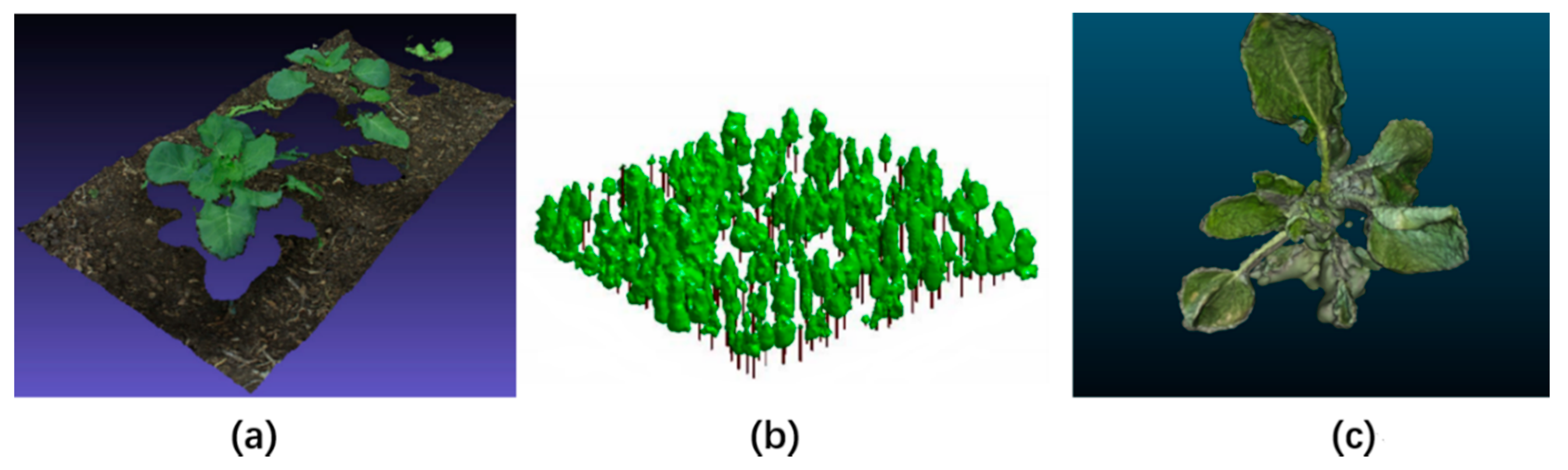
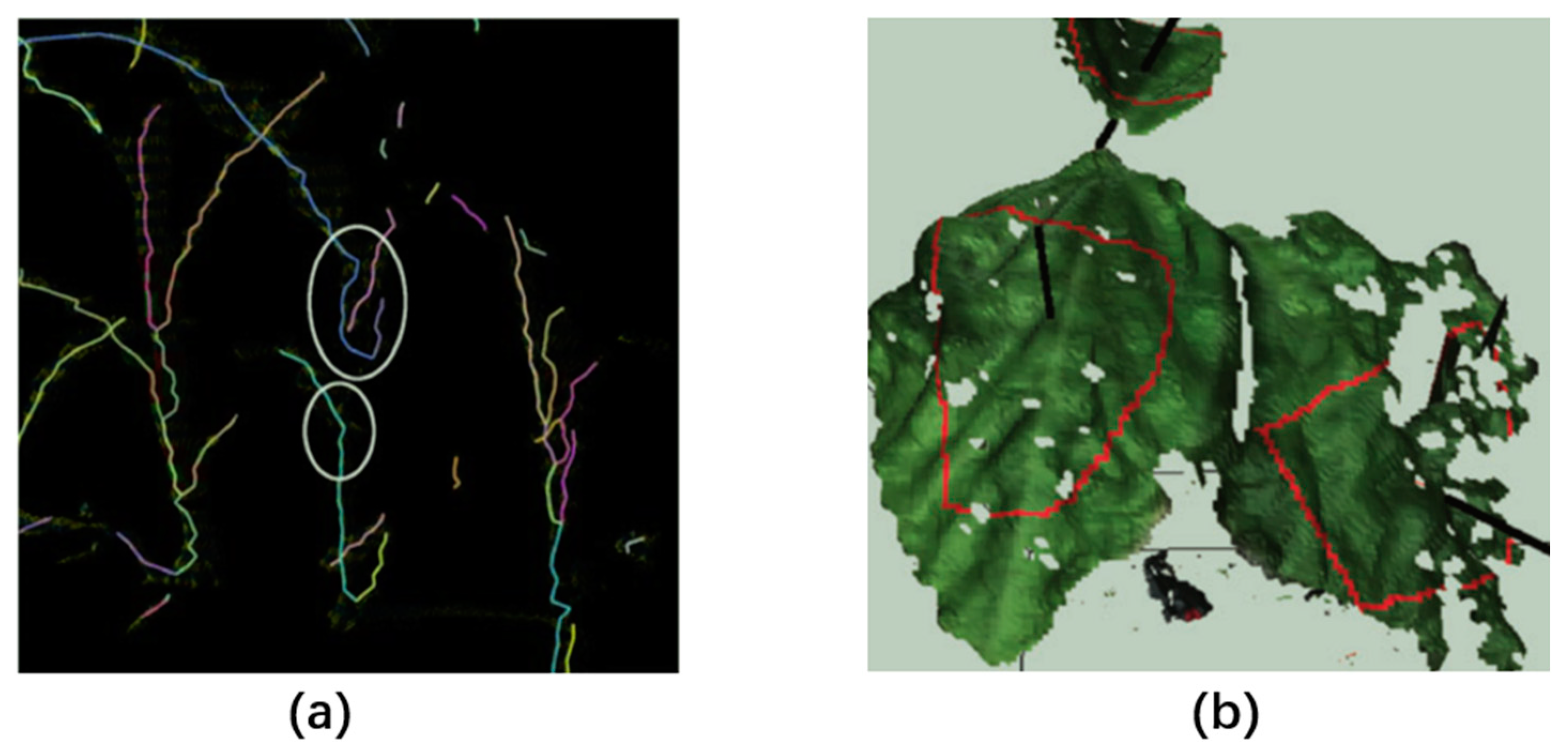
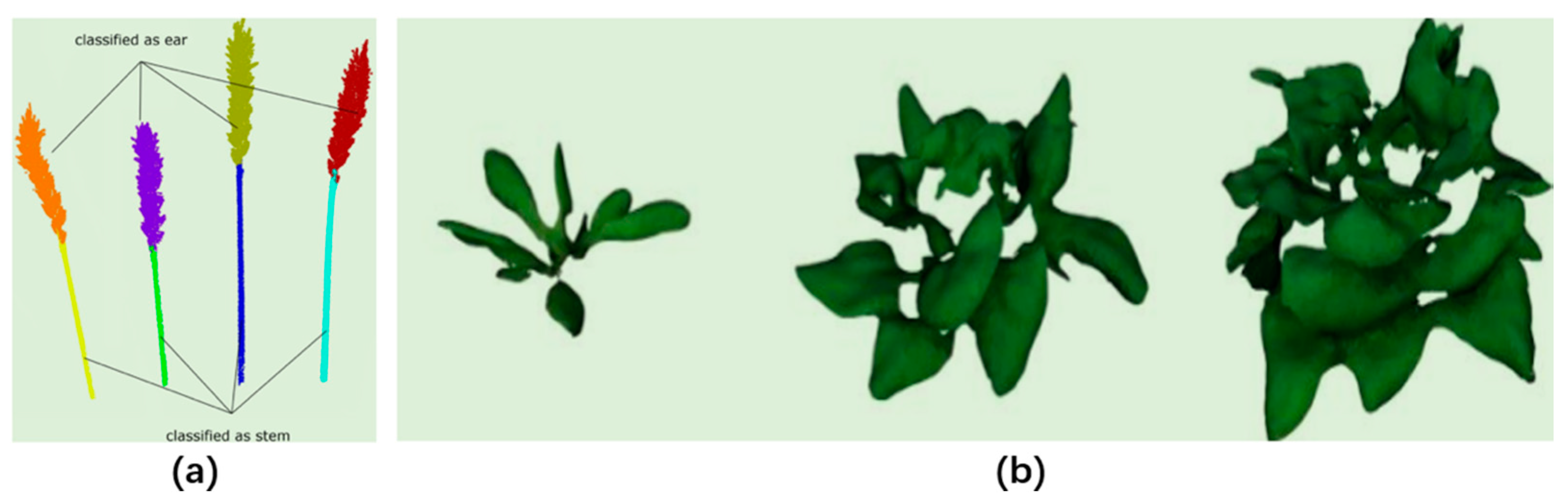
3.4. Plant Canopy Segmentation

Plant canopy study is focused on canopy architecture, leaf angle distribution, leaf morphology, leaf number, leaf size, and so on, so plant leaf point cloud segmentation is necessary before morphological analysis. Plant segmentation is most difficult and important in plant phenotypic analysis, because kinds of plant organ in different vegetation is not similar, which leads to the use of specific methods for different plant segmentation. Three main varieties of range segmentation algorithms are edge-based segmentation, surface-based segmentation, and scanline-based segmentation [98]. The surface-based segmentation methods use local surface properties as a similarity measure and merge together the points that are spatially close and have similar surface properties. Surface-based segmentation is common for plant canopy segmentation and its key is obtaining features for clustering or classification. Spectral clustering algorithm [99] can solve the segmentation problem of plant stem and leaf where the centers and spreads are not an adequate description of the cluster, but the number of clusters must be given as input; Point Feature Histograms (PFH) [100] can better show descriptions of a point’s neighborhood for calculating features. Seed region-growing algorithm [101] is also common for segmentation, it examines neighboring features of initial seed points and determines whether the point should be added to the region, so the selecting of initial seed point is important for the segmentation result.

Paulus [102] proposed a new approach to the segmentation of plant stem and leaf, which applies PFH descriptor into Surface Feature histograms (SFH) in order to make a better distinction, and new descriptors were used as features for labels of machine learning to realize automatic classification. Hu [27] used pot point data to construct a pot shape feature to define plane Sm and segmentation of the plant leaf by whether the point’s projection is or not on plane Sm. Li [103] selected a suitable seed point feature in the K-nearest neighborhood to cluster for coarse planar facer generation, then carried out facet region growing by multiple coarse facers according to facet adjacency and the coplanarity to accomplish leaf segmentation. Dey [104] used saliency features [105] and color data to obtain a 12-dimensional feature vector for each point, then used SVM to classify the point clouds of grape, branches, and leaves according to obtained features. Gélard [106] decomposed 3D point clouds into super-voxel and used the improved region growing approach to segment merged leaves.

Surface fitting benefits plant canopy segmentation, which is used to fit planes or flexible surfaces. Non-uniform rational B-splines (NURBS) [107] algorithm is the general fitting plant leaf surface. Hu et al. [32] proposed an angle of the two adjacent normal vectors method to remove redundant points, and NURBS method was used to fit the plant leaf. Santos [108] used single hand-held to get dense 3D point clouds by MVS technology, sunflower stem and leaf were segmented by spectral clustering algorithm, and leaf surface was estimated using non-uniform rational B-splines (NURBS).

3.5. Plant Canopy Structure Parameters Extraction

Plant structure index is used to characterize growth quality, structural parameters, covering area, and so on. It can be divided into the plant group canopy level [109], individual plant level [110], and plant organ level [111]. The plant canopy plays important functional roles in cycling materials and energy through photosynthesis and transpiration, maintaining plant microclimates, and providing habitats for various taxa [112]. This paper only focuses on the plant group canopy level, which includes leaf inclination angles, leaf area density, plant area density, etc.

3.5.1. Leaf Inclination Angles

The skeleton, also called the symmetry axis, is a useful structure-based object descriptor. Extracting object skeletons directly from natural images can deliver important information about the presence and size of objects. The skeleton segment [113] is often applied to leaf angle measurement. Skeletonization is used to show the geometrical and topological properties of that shape. Bao [30] made a skeleton segmentation for maize and filtered the skeleton nodes that satisfy suitable point-to-stem distance, and leaf angle was computed using PCA and approximated by the first eigenvector of the filtered nodes, the skeleton segmentation result is shown in (a) of Figure 9. As a result of leaf angle stability, not change with zooming in or out, the leaf projected can be used to calculate the leaf angle. Biskup [114] used leaf projected ROI (region of interest) for plane fitting to build a planar surface model, which is obtained by the RANSAC algorithm and by analyzing the covariance matrix of the outlier-free point cloud; the leaf angle was obtained corresponding to the dihedral angle between two planes, the detailed is shown in (b) of Figure 9.

3.5.2. Leaf Area Density (LAD)

Leaf area density (LAD) is defined as the one-sided leaf area per unit of horizontal layer volume [115]. The leaf area index (LAI), which is defined as the leaf area per unit ground area, is calculated by integrating the LAD over the canopy height. For LAD, leaf area and plant volume need to be calculated by each layer voxel area, which is obtained by transferring point clouds into voxel-based three-dimensional model.

For the direct calculating of LAD, Hosoi [116] proposed the voxel-based canopy profiling (VCP) method to estimate tree LAD; data for each horizontal layer of the canopy were collected from optimally inclined laser beams and were converted into a voxel-based three-dimensional model; then LAD and LAI were computed by counting the beam-contact frequency in each layer using a point-quadrat method.

For the measurement of plant volume, an alpha shape volume estimation was used to calculate plant volume [117]. This algorithm estimates the concave hull around point clouds and computes the volume from there. Paulus [102] used an alpha shape volume estimation method for volume estimation and an accurate description of the concave wheat ears with segmental point clouds, the detailed presentation is shown in (a) of Figure 10. Hu [27] proposed a method based on tetrahedrons to calculate plant volume; tetrahedrons were constructed by down-sampled point cloud, distance of any two points should be smaller than maximum edge length of tetrahedrons, and plant volume can be calculated by tetrahedrons point space. When the plant is reconstructed by voxel grid or octree, the volume can be estimated by adding up the volumes of all the voxels covering the plant, the detailed presentation is shown in (b) of Figure 10. Chalidabhongse [118] made 3D mango reconstruction based on the space carving method, and each projected voxel in the voxel space onto the all view of images was the approximation of the object volume.

For leaf fitting using NURBS, leaf area is calculated by the sum of each partial area according to fitting surface mesh. Santos [119] and Hu [32] used NURBS to calculate mint and poplars area, and the results were very accurate. It is relatively simple to get the whole plant area with needless segmentation, Bao [13] converted point clouds into triangle mesh, reconstructed surface with PCL, and the plant surface area was approximated by the sum of areas of all triangles in the mesh. When a voxel grid or octree reconstructs the plant, a sequential cluster connecting algorithm and subsequent refinement steps need to be carried out to segment the leaf, then voxel grid or octree is converted into point cloud for piece-wise fitting of leaf planes [120]. Scharr [55] used volume carving to make 3D maize reconstruction and leaf area was calculated by a sequence of segmentation algorithms. In addition, the marching cubes algorithm [121] can also calculate the area of a voxel or octree by fitting a mesh surface.

3.5.3. Plant Area Density (PAD)

The notion of plant area density (PAD) is easy to understand, which is defined as canopy area per unit of ground area. So the device for generating points of data needs to have a broad-scale survey range, and as such, handheld laser scanner and airborne laser scanner (ALS) remote sensing are often used. As a result of large quantities of data for broad-scale plant area measurement, point cloud segmentation and reconstruction are complex and difficult, so PAD is estimated based on the VCP [116] method by converting point clouds into a voxel-based three-dimensional model. Song [122] used an airborne laser scanner estimate tree PAD, and PAD was computed with the VCP method.

Table 9. Examples of RMSE for plant canopy 3D structure parameters measurement.

RMSE	Cotton [123]	Sunflower [123]	Black Eggplant [123]	Tomato [123]	Maize [30]	Palm Tree Seedling [124]	Leafy Vegetable [27]
Plant height	1.7 cm	1.1 cm	1 cm	1.3 cm	0.058 m	/	0.6957 cm
Leaf area (cm2)	80	30	10	10	/	3.23	72.43
Leaf inclination angles (°)	/	/	/	/	3.455	2.68	/
Stem diameter	/	/	/	/	5.3 mm	/	/
Volume	/	/	/	/	/	/	2.522 cm3

Note: RMSE, root mean square error.

and

Table 10. Examples of MAPE and R2 for plant canopy 3D structure parameters measurement.

	LAD	PAD
Tree	MAPE: 17.2–55.3% [116]	R2: 0.818 [122]

Note: R², Coefficient of determination, the ratio of the sum of the squared regression to the sum of the squared total errors is an index of the degree of fit of the trend line; MAPE, Mean absolute percentage error.

shows the 3D reconstruction of plants and the analysis of the structure index using single and multiple measurement methods.

4. Conclusions

4.1. Poor Standardization of Algorithms

There is a lot of variability of the appearance of different kinds of plants, and the analysis method of reconstruction and segmentation aims to only specific plants, moreover it may apply different algorithms for the same plant in different environments. In the flow of 3D plant data acquisition, point cloud processing, 3D plant reconstruction, plant segmentation, and plant canopy structure parameters extraction have multiple processing algorithms and do not have an optimal criteria to build standards and specifications (such as labeling, naming, formatting, and integrity constraints). The problems include large differences in format and accuracy, incomplete supporting data, data redundancy, and low data use. The data from the plant organ layer to the individual plant layer to the group canopy level are independent from each other in the study of 3D canopy structure, and the matching characterization with plant physiological data (such as canopy photosynthesis data) needs to be standardized [125]. For example, Delaunay triangulation, region-based growth surface reconstruction, and implicit surface reconstruction can be used for plant reconstruction and have different results.

4.2. 3D Reconstruction Operation Is Slow

The data processing speed can be influenced by the number of input points, which could be a time-consuming problem for large-sized plants. When analyzing plant phenotypes on a large scale, 3D reconstruction takes longer and is less efficient due to the large number of objects to be analyzed. The analysis shows that the 3D reconstruction effect of multi-view images is related to the number of images. The higher the number of images, the better the reconstruction effect, but the corresponding calculation amount also increases considerably [126], resulting in a time-consuming reconstruction process. In addition to the speed improvement required by hardware, software algorithms are required to speed up the calculation.

3D reconstruction speed has a direct relationship with point cloud data size, and rough and fine reconstruction also take different times. Marton [127] used the triangulation method to make an urban scene fast surface reconstruction, which needed 8.983 s with 65,646 points and reconstruction of radiohead took 17.857 s with 329,741 points. Although 3D reconstruction takes little time, generating dense and complete a 3D point cloud with multi-images will take a lot of time. The CMPMVS software ran for around 182 min from 66 input images, and Lou [128] used an improved SfM method, which ran for 15 min to produce the final 3D point cloud for the same images.

4.3. Plant 3D Reconstruction Is Inaccurate

Currently, plant analysis and reconstruction technology uses moment phenotype extraction and lacks a monitoring of growth dynamics; however, monitoring of growth dynamics requires a non-invasive time-lapse imaging system that supports accurate reconstruction of plant architecture and most depth cameras or other devices provide only rough approximations of size, often lacking high spatial or high temporal resolution [129]. In addition, the occlusion of the plant canopy structure causes problems such as voids or holes, untextured areas, and blurred images in the final 3D models of some plants. Therefore, occlusion problems should be avoided as much as possible during the image collection process. Multi-view stereo reconstruction with multiple devices working together like laser scanner and ToF camera has high accuracy for sheltered leaves and fruit plant reconstruction, but rapid multi-view registration is difficult for achieving the high-throughput 3D phenotypic analysis.

Models that have been proposed thus far are still limited in their application because of sensitivity to outdoor illumination conditions and the inherent difficulty in modeling complex plant shapes using only radiometric information. Different plant or imaged environments also have a great reconstruction performance difference with the same material and methods. In the 3D stereo model, the reconstruction errors of corn, sunflower, black nightshade, and tomato are 5.7, 4.6, 5.2, and 4.7% in LCA (leaf cover area) [123]. The data accuracy meets the demand for precision agriculture practices, but still needs to improve the reconstruction accuracy in fine phenotypic analysis and texture research.

The process of plant 3D data capture is easily affected by light intensity, blurred edges, wind factors, etc., which lead to data loss or low quality, affecting the segmentation of plants and background. When the plant structure cannot be completely reconstructed, the reconstruction accuracy is reduced. Although when structured light and ToF camera avoid the condition being indoors, having high measuring speed, and strong robustness with a no-movement plant, the major weakness is the existing high noise among 3D data, which is a challenge for plant segmentation. For individual plant organ segmentation, there is no unified and standard methods, which largely vary according to diffident plant morphology. Existing methods based on machine learning can achieve good results, but require manual participation and cannot provide automatic segmentation.

4.4. High Equipment Collection Cost

The current limitation of the broad-scale plant detection is that it relies on a relatively expensive robotic platform and positioning system. The commercial possibilities of a scout robot are better since the robot’s task can be executed while navigating when the automatic data processing can be carried out. As LiDAR [130], light field camera [131], high-precision TOF cameras, and other instruments are expensive, they are suitable only for laboratory research and large-scale facilities and agricultural sites. They are currently in the pilot stage, but manual operation is often needed and the promotion is limited due to funding problems [132]. Although the cost of applying SfM photogrammetry is lower, generating more detailed models will increase time required and costs. For broad-scale plant detection of large farms or forests, airspace carrying devices including unmanned aerial vehicles (UAV) or farm helicopter transport is necessary, which adds the extra cost.

5. Prospection

5.1. Establishing a Standard System of 3D Plant Canopy Structure Data

A future research direction should go into automating the manual estimations by automatically setting the point density parameter in order to avoid manual trimming. Additionally, more research needs to be done with the leaf area index (LAI) parameter estimation. High-throughput phenotyping for large greenhouses and open fields (if the measurements are performed on cloudy or low sunlight intensity days) is a future application for the analysis system. Phenotypical analysts have introduced the canopy structure index into various agricultural professional models to match plant physiological data and improve the international universality of agricultural professional models.

Due to the significant differences in the different plant characteristics on different scales, it is possible to refine the plant species as a unit on multiple scales such as organ, individual, or population, and consider the top-level design principles of 3D structure analysis of plant canopies. The top-level design principles include related terminology categories, detection schemes, technical standards, technical methods, models for obtaining and using relevant data, and the representation and verification procedures of the relationship between various data.

5.2. Speeding Up the 3D Plant Canopy Structure Reconstruction

In the different methods used to study plant phenotype, the effects of image preprocessing and scaling on image registration accuracy can be studied [133] to reduce lighting interference, background interference, image distortion, and other problems, and then improve the matching degree of plant reconstruction and enhance the algorithm robustness. If distributed computing can be combined with computer cluster computing [134], the reconstruction algorithm could be sped up, and performing distributed optimization on the algorithm could also improve the calculation accuracy and reduce the calculation time. Clustering algorithm mainly applies in point clouds processing of background subtraction and outlier removal, along with surface feature-based segmentation.

In the construction of the collection device platform, the UAV is a type of remote sensing platform that is unmanned and reusable. After being equipped with a 3D canopy shape collection device, the UAV could provide rapid collection, flexible movement, and convenient control. Especially with the miniaturization of the 3D shape collection device, UAVs can acquire visible or near-infrared images, 3D point cloud images, multispectral images, and remote sensing images with high spatial resolution at any time. It is possible to construct a 4D space–time scene of farmland based on UAV remote sensing images through real-time data collection to achieve cross-fusion of time series and spatial images [135].

5.3. Improving the Accuracy of the 3D Structure Index of Canopy Reconstruction

3D plant canopy structure measurement technology can be embedded in phenotypical analysis tools. Sensor fusion technology can be used to quantify 3D canopy structure and single leaf shape features by integrating multiple features to improve the accuracy of the structure index. The color, depth, and infrared data included in the image can be combined to improve the integrity of the plant phenotypical data and improve the 3D reconstruction effect. Using multiple devises working together to obtain point clouds from multi-view can reduce noise and improve reconstruction accuracy.

Optimizing the segmentation algorithm parameters to support a wider range of plant species with less parameter tuning is important to improve plant structure index extraction accuracy. Neural networks can be used for classification of segmentation. Deep learning on point clouds is still at the forefront of research. Multi-view convolutional neural networks (CNNs) have tried to render 3D point cloud into 2D images and then apply 2D conv nets to classify them, which can make shape classification, but it cannot achieve 3D tasks such as point classification and shape completion [129]. Feature-based deep convolutional neural networks (DNNs) firstly convert the 3D data into a vector, by extracting traditional shape features and then use a fully connected net to classify the shape, but they are constrained by the representation power of the features extracted [63]. Qi [136] proposed a novel deep neural network called PointNet, it can achieve point classification or semantic segmentation with a 1080X GPU. In conclusion, integrating the local and global features extracted by deep learning models with the spatial representation of the point clouds will be useful to design a model for plant canopy segmentation with top performance, but at present its segmentation quality is low as a result of point clouds being irregular and sparse. The promising solutions are improving multi-scale point clouds resolution, developing the architectures of the deep learning models like those in RGB images, and improving the processing raw point clouds based on zero-shot learning [137].

References

1. Li, D.; Yang, H. State-of-the-art review for internet of things in agriculture. Trans. Chin. Soc. Agric. Mach. 2018, 49, 1–20. [Google Scholar]
2. Rahman, A.; Mo, C.; Cho, B.-K. 3-D image reconstruction techniques for plant and animal morphological analysis—A review. J. Biosyst. Eng. 2017, 42, 339–349. [Google Scholar]
3. Tsai, R. A versatile camera calibration technique for high-accuracy 3D machine vision metrology using off-the-shelf TV cameras and lenses. IEEE J. Robot. Autom. 1987, 3, 323–344. [Google Scholar] [CrossRef] [Green Version]
4. Faugeras, O.; Toscani, G. Camera calibration for 3D computer vision. In Proceedings of the International Workshop on Industrial Application of Machine Vision and Machine Intelligence, Tokyo, Japan, 2–5 February 1987; pp. 240–247. [Google Scholar]
5. Martins, H.; Birk, J.R.; Kelley, R.B. Camera models based on data from two calibration planes. Comput. Gr. Image Process. 1981, 17, 173–180. [Google Scholar] [CrossRef]
6. Pollastri, F. Projection center calibration by motion. Pattern Recognit. Lett. 1993, 14, 975–983. [Google Scholar] [CrossRef]
7. Caprile, B.; Torre, V. Using vanishing points for camera calibration. Int. J. Comput. Vis. 1990, 4, 127–139. [Google Scholar] [CrossRef]
8. Zhang, Z. A flexible new technique for camera calibration. IEEE Trans. Pattern Anal. Mach. Intell. 2000, 22, 1330–1334. [Google Scholar] [CrossRef] [Green Version]
9. Qi, W.; Li, F.; Zhenzhong, L. Review on camera calibration. In Proceedings of the 2010 Chinese Control and Decision Conference, Xuzhou, China, 26–28 May 2010; pp. 3354–3358. [Google Scholar]
10. Andersen, H.J.; Reng, L.; Kirk, K. Geometric plant properties by relaxed stereo vision using simulated annealing. Comput. Electron. Agric. 2005, 49, 219–232. [Google Scholar] [CrossRef]
11. Malekabadi, A.J.; Khojastehpour, M.; Emadi, B. Disparity map computation of tree using stereo vision system and effects of canopy shapes and foliage density. Comput. Electron. Agric. 2019, 156, 627–644. [Google Scholar] [CrossRef]
12. Li, L.; Yu, X.; Zhang, S.; Zhao, X.; Zhang, L. 3D cost aggregation with multiple minimum spanning trees for stereo matching. Appl. Opt. 2017, 56, 3411–3420. [Google Scholar] [CrossRef]
13. Bao, Y.; Tang, L.; Breitzman, M.W.; Salas Fernandez, M.G.; Schnable, P.S. Field-based robotic phenotyping of sorghum plant architecture using stereo vision. J. Field Robot. 2019, 36, 397–415. [Google Scholar] [CrossRef]
14. Baweja, H.S.; Parhar, T.; Mirbod, O.; Nuske, S. Stalknet: A deep learning pipeline for high-throughput measurement of plant stalk count and stalk width. In Field and Service Robotics; Springer: Cham, Switzerland, 2018; pp. 271–284. [Google Scholar]
15. Dandrifosse, S.; Bouvry, A.; Leemans, V.; Dumont, B.; Mercatoris, B. Imaging wheat canopy through stereo vision: Overcoming the challenges of the laboratory to field transition for morphological features extraction. Front. Plant Sci. 2020, 11, 96. [Google Scholar] [CrossRef] [PubMed] [Green Version]
16. Vázquez-Arellano, M.; Griepentrog, H.W.; Reiser, D.; Paraforos, D.S. 3-D imaging systems for agricultural applications—A review. Sensors 2016, 16, 618. [Google Scholar] [CrossRef] [PubMed] [Green Version]
17. Chen, C.; Zheng, Y.F. Passive and active stereo vision for smooth surface detection of deformed plates. IEEE Trans. Ind. Electron. 1995, 42, 300–306. [Google Scholar] [CrossRef]
18. Jin, H.; Soatto, S.; Yezzi, A.J. Multi-view stereo reconstruction of dense shape and complex appearance. Int. J. Comput. Vis. 2005, 63, 175–189. [Google Scholar] [CrossRef] [Green Version]
19. Smith, M.; Carrivick, J.; Quincey, D. Structure from motion photogrammetry in physical geography. Prog. Phys. Geogr. 2016, 40, 247–275. [Google Scholar] [CrossRef]
20. Malambo, L.; Popescu, S.C.; Murray, S.C.; Putman, E.; Pugh, N.A.; Horne, D.W.; Richardson, G.; Sheridan, R.; Rooney, W.L.; Avant, R.; et al. Multitemporal field-based plant height estimation using 3D point clouds generated from small unmanned aerial systems high-resolution imagery. Int. J. Appl. Earth Obs. Geoinf. 2018, 64, 31–42. [Google Scholar] [CrossRef]
21. Tsai, M.; Chiang, K.; Huang, Y.; Lin, Y.; Tsai, J.; Lo, C.; Lin, Y.; Wu, C. The development of a direct georeferencing ready UAV based photogrammetry platform. In Proceedings of the 2010 Canadian Geomatics Conference and Symposium of Commission I, Calgary, AB, Canada, 15–18 June 2010. [Google Scholar]
22. Turner, D.; Lucieer, A.; Wallace, L. Direct georeferencing of ultrahigh-resolution UAV imagery. IEEE Trans. Geosci. Remote Sens. 2013, 52, 2738–2745. [Google Scholar] [CrossRef]
23. Rose, J.; Paulus, S.; Kuhlmann, H. Accuracy analysis of a multi-view stereo approach for phenotyping of tomato plants at the organ level. Sensors 2015, 15, 9651–9665. [Google Scholar] [CrossRef] [Green Version]
24. Süss, A.; Nitta, C.; Spickermann, A.; Durini, D.; Varga, G.; Jung, M.; Brockherde, W.; Hosticka, B.J.; Vogt, H.; Schwope, S. Speed considerations for LDPD based time-of-flight CMOS 3D image sensors. In Proceedings of the 2013 the ESSCIRC (ESSCIRC), Bucharest, Romania, 16–20 September 2013; pp. 299–302. [Google Scholar]
25. Iddan, G.J.; Yahav, G. Three-dimensional imaging in the studio and elsewhere. In Proceedings of the Three-Dimensional Image Capture and Applications IV, San Jose, CA, USA, 13 April 2001; pp. 48–55. [Google Scholar]
26. Foix, S.; Alenya, G.; Torras, C. Lock-in time-of-flight (ToF) cameras: A survey. IEEE Sens. J. 2011, 11, 1917–1926. [Google Scholar] [CrossRef] [Green Version]
27. Hu, Y.; Wang, L.; Xiang, L.; Wu, Q.; Jiang, H. Automatic non-destructive growth measurement of leafy vegetables based on kinect. Sensors 2018, 18, 806. [Google Scholar] [CrossRef] [PubMed] [Green Version]
28. Si, Y.; Wanlin, G.; Jiaqi, M.; Mengliu, W.; Minjuan, W.; Lihua, Z. Method for measurement of vegetable seedlings height based on RGB-D camera. Trans. Chin. Soc. Agric. Mach. 2019, 50, 128–135. [Google Scholar]
29. Vázquez-Arellano, M.; Paraforos, D.S.; Reiser, D.; Garrido-Izard, M.; Griepentrog, H.W. Determination of stem position and height of reconstructed maize plants using a time-of-flight camera. Comput. Electron. Agric. 2018, 154, 276–288. [Google Scholar] [CrossRef]
30. Bao, Y.; Tang, L.; Srinivasan, S.; Schnable, P.S. Field-based architectural traits characterisation of maize plant using time-of-flight 3D imaging. Biosyst. Eng. 2019, 178, 86–101. [Google Scholar] [CrossRef]
31. Liu, S.; Yao, J.; Li, H.; Qiu, C.; Liu, R. Research on 3D skeletal model extraction algorithm of branch based on SR4000. In Journal of Physics: Conference Series; IOP Publishing: Bristol, UK, 2019; p. 022059. [Google Scholar]
32. Hu, C.; Li, P.; Pan, Z. Phenotyping of poplar seedling leaves based on a 3D visualization method. Int. J. Agric. Biol. Eng. 2018, 11, 145–151. [Google Scholar] [CrossRef] [Green Version]
33. Kadambi, A.; Bhandari, A.; Raskar, R. 3d depth cameras in vision: Benefits and limitations of the hardware. In Computer Vision and Machine Learning with RGB-D Sensors; Springer: Cham, Switzerland, 2014; pp. 3–26. [Google Scholar]
34. Verbyla, D.L. Satellite Remote Sensing of Natural Resources; CRC Press: Cleveland, OH, USA, 1995; Volume 4. [Google Scholar]
35. Garrido, M.; Paraforos, D.S.; Reiser, D.; Vázquez Arellano, M.; Griepentrog, H.W.; Valero, C. 3D maize plant reconstruction based on georeferenced overlapping LiDAR point clouds. Remote Sens. 2015, 7, 17077–17096. [Google Scholar] [CrossRef] [Green Version]
36. Shen, D.A.Y.; Liu, H.; Hussain, F. A lidar-based tree canopy detection system development. In Proceedings of the 2018 the 37th Chinese Control Conference (CCC), Wuhan, China, 25–27 July 2018; pp. 10361–10366. [Google Scholar]
37. Shen, Y.; Addis, D.; Liu, H.; Hussain, F. A LIDAR-Based Tree Canopy Characterization under Simulated Uneven Road Condition: Advance in Tree Orchard Canopy Profile Measurement. J. Sens. 2017, 2017, 8367979. [Google Scholar] [CrossRef] [Green Version]
38. Yuan, H.; Bennett, R.S.; Wang, N.; Chamberlin, K.D. Development of a peanut canopy measurement system using a ground-based lidar sensor. Front. Plant Sci. 2019, 10, 203. [Google Scholar] [CrossRef] [Green Version]
39. Qiu, Q.; Sun, N.; Wang, Y.; Fan, Z.; Meng, Z.; Li, B.; Cong, Y. Field-based high-throughput phenotyping for Maize plant using 3D LiDAR point cloud generated with a “Phenomobile”. Front. Plant Sci. 2019, 10, 554. [Google Scholar] [CrossRef] [Green Version]
40. Jin, S.; Su, Y.; Wu, F.; Pang, S.; Gao, S.; Hu, T.; Liu, J.; Guo, Q. Stem–leaf segmentation and phenotypic trait extraction of individual maize using terrestrial LiDAR data. IEEE Trans. Geosci. Remote Sens. 2018, 57, 1336–1346. [Google Scholar] [CrossRef]
41. Geng, J. Structured-light 3D surface imaging: A tutorial. Adv. Opt. Photonics 2011, 3, 128–160. [Google Scholar] [CrossRef]
42. Chéné, Y.; Rousseau, D.; Lucidarme, P.; Bertheloot, J.; Caffier, V.; Morel, P.; Belin, É.; Chapeau-Blondeau, F. On the use of depth camera for 3D phenotyping of entire plants. Comput. Electron. Agric. 2012, 82, 122–127. [Google Scholar] [CrossRef]
43. Azzari, G.; Goulden, M.L.; Rusu, R.B. Rapid characterization of vegetation structure with a Microsoft Kinect sensor. Sensors 2013, 13, 2384–2398. [Google Scholar] [CrossRef] [PubMed] [Green Version]
44. Nguyen, T.; Slaughter, D.; Max, N.; Maloof, J.; Sinha, N. Structured light-based 3D reconstruction system for plants. Sensors 2015, 15, 18587–18612. [Google Scholar] [CrossRef] [Green Version]
45. Syed, T.N.; Jizhan, L.; Xin, Z.; Shengyi, Z.; Yan, Y.; Mohamed, S.H.A.; Lakhiar, I.A. Seedling-lump integrated non-destructive monitoring for automatic transplanting with Intel RealSense depth camera. Artif. Intell. Agric. 2019, 3, 18–32. [Google Scholar] [CrossRef]
46. Vit, A.; Shani, G. Comparing RGB-D sensors for close range outdoor agricultural phenotyping. Sensors 2018, 18, 4413. [Google Scholar] [CrossRef] [Green Version]
47. Liu, J.; Yuan, Y.; Zhou, Y.; Zhu, X.; Syed, T.N. Experiments and analysis of close-shot identification of on-branch citrus fruit with realsense. Sensors 2018, 18, 1510. [Google Scholar] [CrossRef] [Green Version]
48. Milella, A.; Marani, R.; Petitti, A.; Reina, G. In-field high throughput grapevine phenotyping with a consumer-grade depth camera. Comput. Electron. Agric. 2019, 156, 293–306. [Google Scholar] [CrossRef]
49. Perez-Sanz, F.; Navarro, P.J.; Egea-Cortines, M. Plant phenomics: An overview of image acquisition technologies and image data analysis algorithms. GigaScience 2017, 6, gix092. [Google Scholar] [CrossRef] [Green Version]
50. Westoby, M.J.; Brasington, J.; Glasser, N.F.; Hambrey, M.J.; Reynolds, J.M. Structure-from-Motion photogrammetry: A low-cost, effective tool for geoscience applications. Geomorphology 2012, 179, 300–314. [Google Scholar] [CrossRef] [Green Version]
51. Klose, R.; Penlington, J.; Ruckelshausen, A. Usability study of 3D time-of-flight cameras for automatic plant phenotyping. Bornimer Agrartech. Ber. 2009, 69, 12. [Google Scholar]
52. Ma, X.; Zhu, K.; Guan, H.; Feng, J.; Yu, S.; Liu, G. High-throughput phenotyping analysis of potted soybean plants using colorized depth images based on a proximal platform. Remote Sens. 2019, 11, 1085. [Google Scholar] [CrossRef] [Green Version]
53. Sun, G.; Wang, X. Three-dimensional point cloud reconstruction and morphology measurement method for greenhouse plants based on the kinect sensor self-calibration. Agronomy 2019, 9, 596. [Google Scholar] [CrossRef] [Green Version]
54. Paproki, A.; Sirault, X.; Berry, S.; Furbank, R.; Fripp, J. A novel mesh processing based technique for 3D plant analysis. BMC Plant Biol. 2012, 12, 63. [Google Scholar] [CrossRef] [PubMed] [Green Version]
55. Scharr, H.; Briese, C.; Embgenbroich, P.; Fischbach, A.; Fiorani, F.; Müller-Linow, M. Fast high resolution volume carving for 3D plant shoot reconstruction. Front. Plant Sci. 2017, 8, 1680. [Google Scholar] [CrossRef] [Green Version]
56. Kumar, P.; Connor, J.; Mikiavcic, S. High-throughput 3D reconstruction of plant shoots for phenotyping. In Proceedings of the 2014 13th International Conference on Control Automation Robotics and Vision (ICARCV), Singapore, 10–12 December 2014; pp. 211–216. [Google Scholar]
57. Gibbs, J.A.; Pound, M.; French, A.P.; Wells, D.M.; Murchie, E.; Pridmore, T. Plant phenotyping: An active vision cell for three-dimensional plant shoot reconstruction. Plant Physiol. 2018, 178, 524–534. [Google Scholar] [CrossRef] [Green Version]
58. Neubert, B.; Franken, T.; Deussen, O. Approximate image-based tree-modeling using particle flows. In Proceedings of the ACM SIGGRAPH 2007 Papers, San Diego, CA, USA, 5–9 August 2007. [Google Scholar]
59. Aggarwal, A.; Guibas, L.J.; Saxe, J.; Shor, P.W. A linear-time algorithm for computing the Voronoi diagram of a convex polygon. Discret. Comput. Geom. 1989, 4, 591–604. [Google Scholar] [CrossRef]
60. Srihari, S.N. Representation of three-dimensional digital images. ACM Comput. Surv. 1981, 13, 399–424. [Google Scholar] [CrossRef]
61. Vandenberghe, B.; Depuydt, S.; Van Messem, A. How to Make Sense of 3D Representations for Plant Phenotyping: A Compendium of Processing and Analysis Techniques; OSF Preprints: Charlottesville, VA, USA, 2018. [Google Scholar] [CrossRef] [Green Version]
62. Klodt, M.; Herzog, K.; Töpfer, R.; Cremers, D. Field phenotyping of grapevine growth using dense stereo reconstruction. BMC Bioinf. 2015, 16, 143. [Google Scholar] [CrossRef] [Green Version]
63. Guo, K.; Zou, D.; Chen, X. 3D mesh labeling via deep convolutional neural networks. ACM Trans. Graph. 2015, 35, 1–12. [Google Scholar] [CrossRef]
64. Gai, J.; Tang, L.; Steward, B. Plant recognition through the fusion of 2D and 3D images for robotic weeding. In 2015 ASABE Annual International Meeting; American Society of Agricultural and Biological Engineers: St. Joseph, MI, USA, 2015. [Google Scholar]
65. Andújar, D.; Dorado, J.; Fernández-Quintanilla, C.; Ribeiro, A. An approach to the use of depth cameras for weed volume estimation. Sensors 2016, 16, 972. [Google Scholar] [CrossRef] [PubMed] [Green Version]
66. Mitra, N.J.; Nguyen, A. Estimating surface normals in noisy point cloud data. In Proceedings of the Nineteenth Annual Symposium on Computational Geometry, San Diego, CA, USA, 8–10 June 2003; pp. 322–328. [Google Scholar]
67. Hawkins, D.M. Identification of Outliers; Springer: Cham, Switzerland, 1980; Volume 11. [Google Scholar]
68. Johnson, T.; Kwok, I.; Ng, R.T. Fast Computation of 2-Dimensional Depth Contours. In KDD; Citeseer: Princeton, NJ, USA, 1998; pp. 224–228. [Google Scholar]
69. Jain, A.K.; Murty, M.N.; Flynn, P.J. Data clustering: A review. ACM Comput. Surv. 1999, 31, 264–323. [Google Scholar] [CrossRef]
70. Knorr, E.M.; Ng, R.T.; Tucakov, V. Distance-based outliers: Algorithms and applications. VLDB J. 2000, 8, 237–253. [Google Scholar] [CrossRef]
71. Breunig, M.M.; Kriegel, H.-P.; Ng, R.T.; Sander, J. LOF: Identifying density-based local outliers. In Proceedings of the 2000 ACM SIGMOD International Conference on Management of Data, Dallas, TX, USA, 16–18 May 2000; pp. 93–104. [Google Scholar]
72. Fleishman, S.; Cohen-Or, D.; Silva, C.T. Robust moving least-squares fitting with sharp features. ACM Trans. Graph. 2005, 24, 544–552. [Google Scholar] [CrossRef]
73. Wu, J.; Xue, X.; Zhang, S.; Qin, W.; Chen, C.; Sun, T. Plant 3D reconstruction based on LiDAR and multi-view sequence images. Int. J. Precis. Agric. Aviat. 2018, 1. [Google Scholar] [CrossRef]
74. Wolff, K.; Kim, C.; Zimmer, H.; Schroers, C.; Botsch, M.; Sorkine-Hornung, O.; Sorkine-Hornung, A. Point cloud noise and outlier removal for image-based 3D reconstruction. In Proceedings of the 2016 the Fourth International Conference on 3D Vision (3DV), Stanford, CA, USA, 25–28 October 2016; pp. 118–127. [Google Scholar]
75. Xia, C.; Shi, Y.; Yin, W. Obtaining and denoising method of three-dimensional point cloud data of plants based on TOF depth sensor. Trans. Chin. Soc. Agric. Eng. 2018, 34, 168–174. [Google Scholar]
76. Zhou, Z.; Chen, B.; Zheng, G.; Wu, B.; Miao, X.; Yang, D.; Xu, C. Measurement of vegetation phenotype based on ground-based lidar point cloud. J. Ecol. 2020, 39, 308–314. [Google Scholar]
77. Besl, P.J.; McKay, N.D. Method for registration of 3-D shapes. In Proceedings of the Sensor Fusion IV: Control Paradigms and Data Structures, Boston, MA, USA, 30 April 1992; pp. 586–606. [Google Scholar]
78. Jian, B.; Vemuri, B.C. A robust algorithm for point set registration using mixture of Gaussians. In Proceedings of the Tenth IEEE International Conference on Computer Vision (ICCV’05), Beijing, China, 17–21 October 2005; Volume 1, pp. 1246–1251. [Google Scholar]
79. Chui, H.; Rangarajan, A. A new point matching algorithm for non-rigid registration. Comput. Vis. Image Underst. 2003, 89, 114–141. [Google Scholar] [CrossRef]
80. Jia, H.; Meng, Y.; Xing, Z.; Zhu, B.; Peng, X.; Ling, J. 3D model reconstruction of plants based on point cloud stitching. Appl. Sci. Technol. 2019, 46, 19–24. [Google Scholar]
81. Boissonnat, J.-D. Geometric structures for three-dimensional shape representation. ACM Trans. Graph. 1984, 3, 266–286. [Google Scholar] [CrossRef]
82. Curless, B.; Levoy, M. A volumetric method for building complex models from range images. In Proceedings of the 23rd Annual Conference on Computer Graphics and Interactive Techniques, New York, NY, USA, 4–9 August 1996; pp. 303–312. [Google Scholar]
83. Edelsbrunner, H.; Mücke, E.P. Three-dimensional alpha shapes. ACM Trans. Graph. 1994, 13, 43–72. [Google Scholar] [CrossRef]
84. Amenta, N.; Choi, S.; Dey, T.K.; Leekha, N. A simple algorithm for homeomorphic surface reconstruction. In Proceedings of the Sixteenth Annual Symposium on Computational Geometry, Kowloon, Hong Kong, China, 12–14 June 2000; pp. 213–222. [Google Scholar]
85. Forero, M.G.; Gomez, F.A.; Forero, W.J. Reconstruction of surfaces from points-cloud data using Delaunay triangulation and octrees. In Proceedings of the Vision Geometry XI, Seattle, WA, USA, 24 November 2002; pp. 184–194. [Google Scholar]
86. Liang, J.; Park, F.; Zhao, H. Robust and efficient implicit surface reconstruction for point clouds based on convexified image segmentation. J. Sci. Comput. 2013, 54, 577–602. [Google Scholar] [CrossRef]
87. Carr, J.C.; Beatson, R.K.; Cherrie, J.B.; Mitchell, T.J.; Fright, W.R.; McCallum, B.C.; Evans, T.R. Reconstruction and representation of 3D objects with radial basis functions. In Proceedings of the 28th Annual ACM Conference on Computer Graphics and Interactive Techniques, Los Angeles, CA, USA, 12–17 August 2001; pp. 67–76. [Google Scholar]
88. Alexa, M.; Behr, J.; Cohen-Or, D.; Fleishman, S.; Levin, D.; Silva, C.T. Point set surfaces. In Proceedings of the IEEE Conference on Visualization ’01, San Diego, CA, USA, 21–26 October 2001; pp. 21–28. [Google Scholar]
89. Ohtake, Y.; Belyaev, A.; Alexa, M.; Turk, G.; Seidel, H.-P. Multi-level partition of unity implicits. In ACM Siggraph 2005 Courses; Association for Computing Machinery: New York, NY, USA, 2005. [Google Scholar]
90. Kazhdan, M.; Bolitho, M.; Hoppe, H. Poisson surface reconstruction. In Proceedings of the Fourth Eurographics Symposium on Geometry Processing, Cagliari, Sardinia, Italy, 26–28 June 2006; Eurographics Association: Goslar, Germany, 2006; pp. 60–66. [Google Scholar]
91. Boissonnat, J.-D.; Flototto, J. A local coordinate system on a surface. In Proceedings of the Seventh ACM Symposium on Solid Modeling and Applications, Saarbrücken, Germany, 17–21 June 2002; pp. 116–126. [Google Scholar]
92. Jay, S.; Rabatel, G.; Hadoux, X.; Moura, D.; Gorretta, N. In-field crop row phenotyping from 3D modeling performed using Structure from Motion. Comput. Electron. Agric. 2015, 110, 70–77. [Google Scholar] [CrossRef] [Green Version]
93. Andújar, D.; Ribeiro, A.; Fernández-Quintanilla, C.; Dorado, J. Using depth cameras to extract structural parameters to assess the growth state and yield of cauliflower crops. Comput. Electron. Agric. 2016, 122, 67–73. [Google Scholar] [CrossRef]
94. Martinez-Guanter, J.; Ribeiro, Á.; Peteinatos, G.G.; Pérez-Ruiz, M.; Gerhards, R.; Bengochea-Guevara, J.M.; Machleb, J.; Andújar, D. Low-cost three-dimensional modeling of crop plants. Sensors 2019, 19, 2883. [Google Scholar] [CrossRef] [PubMed] [Green Version]
95. Hu, P.; Guo, Y.; Li, B.; Zhu, J.; Ma, Y. Three-dimensional reconstruction and its precision evaluation of plant architecture based on multiple view stereo method. Trans. Chin. Soc. Agric. Eng. 2015, 31, 209–214. [Google Scholar]
96. Pound, M.P.; French, A.P.; Murchie, E.H.; Pridmore, T.P. Automated recovery of three-dimensional models of plant shoots from multiple color images. Plant. Physiol. 2014, 166, 1688–1698. [Google Scholar] [CrossRef] [Green Version]
97. Kato, A.; Schreuder, G.F.; Calhoun, D.; Schiess, P.; Stuetzle, W. Digital surface model of tree canopy structure from LIDAR data through implicit surface reconstruction. In Proceedings of the ASPRS 2007 Annual Conference, Tampa, FL, USA, 7–11 May 2007; Citeseer: Princeton, NJ, USA, 2007. [Google Scholar]
98. Tahir, R.; Heuvel, F.V.D.; Vosselmann, G. Segmentation of point clouds using smoothness constraint. Int. Arch. Photogramm. Remote Sens. SPATIAL Inf. Sci. 2006, 36, 248–253. [Google Scholar]
99. Ng, A.Y.; Jordan, M.I.; Weiss, Y. On spectral clustering: Analysis and an algorithm. In Advances in Neural Information Processing Systems; MIT Press: Cambridge, MA, USA, 2002; pp. 849–856. [Google Scholar]
100. Rusu, R.B.; Blodow, N.; Marton, Z.C.; Beetz, M. Aligning point cloud views using persistent feature histograms. In Proceedings of the 2008 IEEE/RSJ International Conference on Intelligent Robots and Systems, Nice, France, 22–26 September 2008; pp. 3384–3391. [Google Scholar]
101. Mehnert, A.; Jackway, P. An improved seeded region growing algorithm. Pattern Recognit. Lett. 1997, 18, 1065–1071. [Google Scholar] [CrossRef]
102. Paulus, S.; Dupuis, J.; Mahlein, A.-K.; Kuhlmann, H. Surface feature based classification of plant organs from 3D laserscanned point clouds for plant phenotyping. BMC Bioinf. 2013, 14, 238. [Google Scholar] [CrossRef] [Green Version]
103. Li, D.; Cao, Y.; Tang, X.-S.; Yan, S.; Cai, X. Leaf segmentation on dense plant point clouds with facet region growing. Sensors 2018, 18, 3625. [Google Scholar] [CrossRef] [PubMed] [Green Version]
104. Dey, D.; Mummert, L.; Sukthankar, R. Classification of plant structures from uncalibrated image sequences. In Proceedings of the 2012 IEEE Workshop on the Applications of Computer Vision (WACV), Breckenridge, CO, USA, 9–11 January 2012; pp. 329–336. [Google Scholar]
105. Lalonde, J.F.; Vandapel, N.; Huber, D.F.; Hebert, M. Natural terrain classification using three-dimensional ladar data for ground robot mobility. J. Field Robot. 2006, 23, 839–861. [Google Scholar] [CrossRef]
106. Gélard, W.; Herbulot, A.; Devy, M.; Debaeke, P.; McCormick, R.F.; Truong, S.K.; Mullet, J. Leaves segmentation in 3d point cloud. In International Conference on Advanced Concepts for Intelligent Vision Systems; Springer: Cham, Switzerland, 2017; pp. 664–674. [Google Scholar]
107. Piegl, L.; Tiller, W. Symbolic operators for NURBS. Comput. Aided Design 1997, 29, 361–368. [Google Scholar] [CrossRef]
108. Santos, T.T.; Koenigkan, L.V.; Barbedo, J.G.A.; Rodrigues, G.C. 3D plant modeling: Localization, mapping and segmentation for plant phenotyping using a single hand-held camera. In European Conference on Computer Vision; Springer: Cham, Switzerland, 2014; pp. 247–263. [Google Scholar]
109. Müller-Linow, M.; Pinto-Espinosa, F.; Scharr, H.; Rascher, U. The leaf angle distribution of natural plant populations: Assessing the canopy with a novel software tool. Plant Methods 2015, 11, 11. [Google Scholar] [CrossRef] [Green Version]
110. Zhu, B.; Liu, F.; Zhu, J.; Guo, Y.; Ma, Y. Three-dimensional quantifications of plant growth dynamics in field-grown plants based on machine vision method. Trans. Chin. Soc. Agric. Mach. 2018, 49, 256–262. [Google Scholar]
111. Sodhi, P.; Hebert, M.; Hu, H. In-Field Plant Phenotyping Using Model-Free and Model-Based Methods. Master’s Thesis, Carnegie Mellon University Pittsburgh, Pittsburgh, PA, USA, 2017. [Google Scholar]
112. Hosoi, F.; Omasa, K. Estimating vertical plant area density profile and growth parameters of a wheat canopy at different growth stages using three-dimensional portable lidar imaging. ISPRS J. Photogramm. Remote Sens. 2009, 64, 151–158. [Google Scholar] [CrossRef]
113. Cornea, N.D.; Silver, D.; Min, P. Curve-skeleton properties, applications, and algorithms. IEEE Trans. Vis. Comput. Graph. 2007, 13, 530. [Google Scholar] [CrossRef] [Green Version]
114. Biskup, B.; Scharr, H.; Schurr, U.; Rascher, U. A stereo imaging system for measuring structural parameters of plant canopies. Plant Cell Environ. 2007, 30, 1299–1308. [Google Scholar] [CrossRef]
115. Weiss, M.; Baret, F.; Smith, G.; Jonckheere, I.; Coppin, P. Review of methods for in situ leaf area index (LAI) determination: Part II. Estimation of LAI, errors and sampling. Agric. For. Meteorol. 2004, 121, 37–53. [Google Scholar] [CrossRef]
116. Hosoi, F.; Omasa, K. Voxel-based 3-D modeling of individual trees for estimating leaf area density using high-resolution portable scanning lidar. IEEE Trans. Geosci. Remote Sens. 2006, 44, 3610–3618. [Google Scholar] [CrossRef]
117. Liang, J.; Edelsbrunner, H.; Fu, P.; Sudhakar, P.V.; Subramaniam, S. Analytical shape computation of macromolecules: I. Molecular area and volume through alpha shape. Proteins Struct. Function Bioinf. 1998, 33, 1–17. [Google Scholar] [CrossRef]
118. Chalidabhongse, T.; Yimyam, P.; Sirisomboon, P. 2D/3D vision-based mango’s feature extraction and sorting. In Proceedings of the 2006 the 9th International Conference on Control, Automation, Robotics and Vision, Singapore, 5–8 December 2006; pp. 1–6. [Google Scholar]
119. SANTOS, T.; Ueda, J. Automatic 3D plant reconstruction from photographies, segmentation and classification of leaves and internodes using clustering. In Embrapa Informática Agropecuária-Resumo em anais de congresso (ALICE); Finnish Society of Forest Science: Vantaa, Finland, 2013. [Google Scholar]
120. Embgenbroich, P. Bildbasierte Entwicklung Eines Dreidimensionalen Pflanzenmodells am Beispiel von Zea Mays. Master’s Thesis, Helmholtz Association of German Research Centers, Berlin, Germany, 2015. [Google Scholar]
121. Lorensen, W.E.; Cline, H.E. Marching cubes: A high resolution 3D surface construction algorithm. ACM Siggraph Comput. Graph. 1987, 21, 163–169. [Google Scholar] [CrossRef]
122. Song, Y.; Maki, M.; Imanishi, J.; Morimoto, Y. Voxel-based estimation of plant area density from airborne laser scanner data. Int. Arch. Photogramm. Remote Sens. Spat. Inf. Sci. 2011, 38, W12. [Google Scholar] [CrossRef] [Green Version]
123. Lati, R.N.; Filin, S.; Eizenberg, H. Plant growth parameter estimation from sparse 3D reconstruction based on highly-textured feature points. Precis. Agric. 2013, 14, 586–605. [Google Scholar] [CrossRef]
124. Itakura, K.; Hosoi, F. Automatic leaf segmentation for estimating leaf area and leaf inclination angle in 3D plant images. Sensors 2018, 18, 3576. [Google Scholar] [CrossRef] [Green Version]
125. Zhao, C. Big data of plant phenomics and its research progress. J. Agric. Big Data 2019, 1, 5–14. [Google Scholar]
126. Zhou, J.; Guo, X.; Wu, S.; Du, J.; Zhao, C. Research progress on 3D reconstruction of plants based on multi-view images. China Agric. Sci. Technol. Rev. 2018, 21, 9–18. [Google Scholar]
127. Marton, Z.C.; Rusu, R.B.; Beetz, M. On fast surface reconstruction methods for large and noisy point clouds. In Proceedings of the 2009 IEEE International Conference on Robotics and Automation, Kobe, Japan, 12–17 May 2009; pp. 3218–3223. [Google Scholar]
128. Lou, L.; Liu, Y.; Han, J.; Doonan, J.H. Accurate multi-view stereo 3D reconstruction for cost-effective plant phenotyping. In International Conference Image Analysis and Recognition; Springer: Cham, Switzerland, 2014; pp. 349–356. [Google Scholar]
129. Apelt, F.; Breuer, D.; Nikoloski, Z.; Stitt, M.; Kragler, F. Phytotyping4D: A light-field imaging system for non-invasive and accurate monitoring of spatio-temporal plant growth. Plant J. 2015, 82, 693–706. [Google Scholar] [CrossRef]
130. Itakura, K.; Hosoi, F. Estimation of leaf inclination angle in three-dimensional plant images obtained from lidar. Remote Sens. 2019, 11, 344. [Google Scholar] [CrossRef] [Green Version]
131. Zhao, J.; Liu, Z.; Guo, B. Three-dimensional digital image correlation method based on a light field camera. Opt. Lasers Eng. 2019, 116, 19–25. [Google Scholar] [CrossRef]
132. Hu, Y. Research on Three-Dimensional Reconstruction and Growth Measurement of Leafy Crops based on Depth Camera; Zhejiang University: Hangzhou, China, 2018. [Google Scholar]
133. Henke, M.; Junker, A.; Neumann, K.; Altmann, T.; Gladilin, E. Automated alignment of multi-modal plant images using integrative phase correlation approach. Front. Plant Sci. 2018, 9, 1519. [Google Scholar] [CrossRef] [PubMed] [Green Version]
134. Myint, K.N.; Aung, W.T.; Zaw, M.H. Research and analysis of parallel performance with MPI odd-even sorting algorithm on super cheap computing cluster. In Seventeenth International Conference on Computer Applications; University of Computer Studies, Yangon under Ministry of Education: Yangon, Myanmar, 2019; pp. 99–106. [Google Scholar]
135. Dong, J.; Burnham, J.G.; Boots, B.; Rains, G.; Dellaert, F. 4D crop monitoring: Spatio-temporal reconstruction for agriculture. In Proceedings of the 2017 IEEE International Conference on Robotics and Automation (ICRA), Singapore, 29 May–3 June 2017; pp. 3878–3885. [Google Scholar]
136. Qi, C.R.; Su, H.; Mo, K.; Guibas, L.J. Pointnet: Deep learning on point sets for 3d classification and segmentation. In Proceedings of the IEEE Conference on Computer Vision and Pattern Recognition, Honolulu, HI, USA, 21–26 July 2017; pp. 652–660. [Google Scholar]
137. Liu, W.; Sun, J.; Li, W.; Hu, T.; Wang, P. Deep learning on point clouds and its application: A survey. Sensors 2019, 19, 4188. [Google Scholar] [CrossRef] [PubMed] [Green Version]
Figure 1. Binocular stereo vision principle. x1 and x2 is value of image coordinate and can be obtained from image plane directly, and camera calibration can get f (focal distance) and b (baseline). The z (deep of object) can be calculated by triangle similarity principle, which result as z = f b x 1 x 2 , and x and y can be calculated by z and image plane coordinate.
Agriculture 10 00462 g001
Figure 2. Principle of time of flight image collection: (a) distance measurement based on continuous-wave modulation; (b) distance measurement based on pulsed modulation.
Agriculture 10 00462 g002
Figure 3. The principle of structured light.
Agriculture 10 00462 g003
Figure 4. Flow chart of plant canopy structure measurement based on 3D reconstruction.
Agriculture 10 00462 g004
Figure 5. Data type: (a) depth maps, (b) polygon meshes, (c) voxels, and (d) 3D point clouds.
Agriculture 10 00462 g005
Figure 6. Result after ground removal with Random Sample Consensus (RANSAC) [64].
Agriculture 10 00462 g006
Figure 7. Iterative closest point (ICP) algorithm: realize the registration of A and B point clouds.
Agriculture 10 00462 g007
Figure 8. (a) Cabbage reconstruction based on Delaunay triangulation [92]; (b) Tree reconstruction based on implicit surface reconstruction algorithm [97]; (c) Sugar beet reconstruction based on Poisson algorithm [94].
Agriculture 10 00462 g008
Figure 9. (a) Skeleton segments that contain both stems and leaves [30]; (b) 3D reconstruction of a soybean leaf consisting of three leaflets. Black lines: normal vectors to fitted plane; red contour: projected region of interest (ROI) used for plane fitting [114].
Agriculture 10 00462 g009
Figure 10. (a) A description of the concave wheat ears with segmental point clouds [102]; (b) The triangulation results of three different sized plants, and the triangle vertexes extracted from triangular mesh were used as the points to construct tetrahedrons, which can be used to calculate volume [27].
Agriculture 10 00462 g010